Electron Transport through T-Shaped Double-Dots System

1 Introduction

Recent intensive investigations of electron transport phenomena through quantum dot systems have revealed that the strong electron-electron interaction plays a crucial role at low temperatures. In particular, the Kondo effect, which is a prototypical many-body effect, has been discovered in a single-dot system, stimulating further theoretical and experimental studies.${}^{\hbox{\immediate{\bf{?}},\penalty 1000\hskip 0.91003pt plus 0.70004pt minus 0.70004pt{\bf{?}},\penalty 1000\hskip 0.91003pt plus 0.70004pt minus 0.70004pt{\bf{?}},\penalty 1000\hskip 0.91003pt plus 0.70004pt minus 0.70004pt{\bf{?}},\penalty 1000\hskip 0.91003pt plus 0.70004pt minus 0.70004pt{\bf{?}},\penalty 1000\hskip 0.91003pt plus 0.70004pt minus 0.70004pt{\bf{?}},\penalty 1000\hskip 0.91003pt plus 0.70004pt minus 0.70004pt{\bf{?}},\penalty 1000\hskip 0.91003pt plus 0.70004pt minus 0.70004pt{\bf{?}},\penalty 1000\hskip 0.91003pt plus 0.70004pt minus 0.70004pt{\bf{?}},\penalty 1000\hskip 0.91003pt plus 0.70004pt minus 0.70004pt{\bf{?}})}}$ The Kondo effect has been also observed in coupled quantum dots,${}^{\hbox{\immediate{\bf{?}},\penalty 1000\hskip 0.91003pt plus 0.70004pt minus 0.70004pt{\bf{?}},\penalty 1000\hskip 0.91003pt plus 0.70004pt minus 0.70004pt{\bf{?}},\penalty 1000\hskip 0.91003pt plus 0.70004pt minus 0.70004pt{\bf{?}})}}$ in which the inter-dot coupling is coulombly controllable, making this system especially fascinating. In particular, from systematic studies on coupled quantum dots it has been pointed out that a wide variety of Kondo-like phenomena can indeed occur at low temperatures.${}^{\hbox{\immediate{\bf{?}},\penalty 1000\hskip 0.91003pt plus 0.70004pt minus 0.70004pt{\bf{?}},\penalty 1000\hskip 0.91003pt plus 0.70004pt minus 0.70004pt{\bf{?}},\penalty 1000\hskip 0.91003pt plus 0.70004pt minus 0.70004pt{\bf{?}},\penalty 1000\hskip 0.91003pt plus 0.70004pt minus 0.70004pt{\bf{?}},\penalty 1000\hskip 0.91003pt plus 0.70004pt minus 0.70004pt{\bf{?}})}}$

There has been another remarkable phenomenon observed in quantum dot systems, i.e. the Fano effect,${}^{\hbox{\immediate{\bf{?}},\penalty 1000\hskip 0.91003pt plus 0.70004pt minus 0.70004pt{\bf{?}},\penalty 1000\hskip 0.91003pt plus 0.70004pt minus 0.70004pt{\bf{?}},\penalty 1000\hskip 0.91003pt plus 0.70004pt minus 0.70004pt{\bf{?}})}}$ which is caused by the interference between two distinct resonant channels in the tunneling process. When this effect is combined with the Kondo effect, it may provide various interesting many-body effects by the interplay of both phenomena.

In this paper, we investigate tunneling phenomena through a system of two coupled quantum dots in specific parallel-geometry shown in Fig.1, which may be referred to as a system of T-shaped double dots. The system is also regarded as a single-dot system decollated by another dot, so that the additional right dot may open a tunneling channel distinct from the direct resonance via the left dot, and is thus expected to give rise to the interplay between the Kondo effect and the Fano-type interference effect. By using non-crossing approximation (NCA) ${}^{\hbox{\immediate{\bf{?}},\penalty 1000\hskip 0.91003pt plus 0.70004pt minus 0.70004pt{\bf{?}},\penalty 1000\hskip 0.91003pt plus 0.70004pt minus 0.70004pt{\bf{?}},\penalty 1000\hskip 0.91003pt plus 0.70004pt minus 0.70004pt{\bf{?}},\penalty 1000\hskip 0.91003pt plus 0.70004pt minus 0.70004pt{\bf{?}})}}$ approach for a generalized Anderson tunneling Hamiltonian, we calculate the local density of states (DOS) and the tunneling conductance. The NCA approach is further supplemented by the zero-temperature calculation by means of slave-boson mean field (SBMF) approximation.${}^{\hbox{\immediate{\bf{?}},\penalty 1000\hskip 0.91003pt plus 0.70004pt minus 0.70004pt{\bf{?}})}}$ We discuss how several tunable parameters influence the local DOS and the tunneling conductance. It is shown that the inter-dot coupling and the relative position of dot levels play an essential role for electron transport. In particular, we find that in the Kondo regime with a small inter-dot tunneling, the Kondo-mediated conductance is suppressed by the Fano-like interference effect.

This paper is organized as follows. In the next section, we briefly describe the model and the method, and then in §3 we show the results obtained for the local DOS and the conductance. A brief summary is given in §4

2 Model and Method

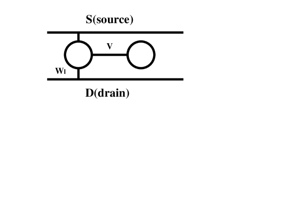
Fig.  1: T-shaped double-dots system in parallel geometry. The left dot is connected to both of the leads whereas the right dot is to the left one. The tunneling amplitude between the dots is $V$ and that between the left dot and the leads is $W_{l}$.

2.1 Model Hamiltonian

We consider T-shaped double dots shown in Fig. 1. This system is described by an extended Anderson Hamiltonian for double dots,

$$H =H_{loc}+H_{mix}$$ (1)

$$H {}_{loc}=\sum_{i=l,r}\sum_{\sigma}\epsilon_{i}d_{i\sigma}^{\dagger}d_{i\sigma}+V\sum_{i\neq j}d_{i\sigma}^{\dagger}d_{i\sigma}+U\sum_{i}n_{i\uparrow}n_{i\downarrow}$$

$$H {}_{med}=\sum_{k\sigma\alpha}\epsilon_{k\sigma\alpha}c_{k\sigma\alpha}^{\dagger}c_{k\sigma\alpha}+\frac{1}{\sqrt{2}}\sum_{k\sigma\alpha}(W_{l}c_{k\sigma\alpha}^{\dagger}d_{l\sigma}+h.c)$$

where $d_{i\sigma}^{\dagger}$ creates an electron in the left or right dot (labeled by $i=l,r$) with the energy $\epsilon_{i}$ and spin $\sigma$, whereas $c_{k\sigma\alpha}^{\dagger}$ creates an electron in the leads specified by $\alpha=s,d$ (source, drain) with the energy $\epsilon_{k\sigma\alpha}$ and spin $\sigma$. $V$ is the inter-dot tunneling amplitude while $W_{l}$ is that between the left dot and the leads. We assume that the intra-dot Coulomb interaction is sufficiently large to prohibit the double occupancy of electrons in each dot. To treat this situation, we apply the NCA to our model, which is known to give reasonable results in the temperature range larger than the Kondo temperature.${}^{\hbox{\immediate{?},\penalty 1000\hskip 0.91003pt plus 0.70004pt minus 0.70004pt{?},\penalty 1000\hskip 0.91003pt plus 0.70004pt minus 0.70004pt{?})}}$ At lower temperatures the NCA may become inappropriate so that we adopt a complementary approach based on the SBMF approximation at zero temperature.${}^{\hbox{\immediate{?},\penalty 1000\hskip 0.91003pt plus 0.70004pt minus 0.70004pt{?})}}$

2.2 NCA approach

Let us treat the Hamiltonian (1) by extending the NCA to the case possessing several kinds of ionic propagators. A similar extension of the NCA to the case of four ionic propagators has been applied successfully to the single impurity Anderson model with the finite Coulomb interaction.${}^{\hbox{\immediate{?})}}$ In order to formulate the Green function for our double-dots model, we first diagonalize the local Hamiltonian $H_{loc}$, which can be expressed in terms of the Hubbard operators $X_{mn}=|m\rangle\langle n|$ as

$$H_{loc}=\sum_{m=1}^{9}E_{m}X_{mm},$$ (2)

where $|m\rangle$ and $E_{m}$ respectively denote the eigenstate of the local Hamiltonian and the corresponding eigenenergy. Recall that we should impose the constraint on the Hilbert space such that double occupancy of electrons in each dot is forbidden. The remaining Hamiltonian $H_{med}$ can be also expressed in terms of the Hubbard operators as

$$H_{med} = \sum_{k\sigma\alpha}\epsilon_{k\sigma\alpha}c_{k\sigma\alpha}^{\dagger}c_{k\sigma\alpha}$$ (3)

$$+ \frac{1}{\sqrt{2}}\sum_{k\sigma\alpha}\sum_{mn}(W_{l}U_{nm}^{l\sigma*}c_{k\sigma\alpha}^{\dagger}X_{nm}+h.c),$$

where the matrix element $U_{nm}^{l\sigma}$ is given by

$$U_{nm}^{l\sigma}=\langle m|d_{l\sigma}^{\dagger}|n\rangle.$$ (4)

For each eigenstate $|m\rangle$, the ionic propagator and the corresponding local DOS are defined by

$$P_{m}(\omega)=\frac{1}{\omega-E_{m}-\Sigma_{m}(\omega)},$$ (5)

$$\rho_{m}(\omega)=-\frac{1}{\pi}{\rm Im}P_{m}(\omega+{\rm i}\delta),$$ (6)

and its self-energy is represented in terms of $U_{nm}^{l\sigma}$ as

$$\Sigma_{m}(\omega) = \sum_{n\sigma}(|U_{mn}^{l\sigma}|^{2}+|U_{nm}^{l\sigma}|^{2})$$ (7)

$$\times \Delta\int_{-\infty}^{\infty}{\rm d}\epsilon f(\eta_{mn}\epsilon)P_{n}(\omega+\eta_{mn}\epsilon)$$

where $f(\epsilon)=[\exp(\beta\epsilon)+1]^{-1}$ is the Fermi distribution function ($\beta=1/T$), and we set $\eta_{mn}=-1(+1)$ if the number of particles accommodated in $|m\rangle$ is larger (smaller) than that in $|n\rangle$. We evaluate the self-energy $\Sigma_{m}(\omega)$ in a self-consistent perturbation theory up to the second order in the hybridization $W_{l}$ as is usually done in the NCA. The left and right Green’s functions are given by

$$G_{l(r)}(\omega)=\sum_{mn}|U_{mn}^{l(r)\sigma}|^{2}\langle\langle X_{mn};X_{nm}\rangle\rangle_{\omega},$$ (8)

$$\langle\langle X_{mn} X_{nm}\rangle\rangle_{\omega}$$ ; (9)

$$= \frac{1}{Z_{loc}}\int{\rm d}\epsilon e^{-\beta\epsilon}[\rho_{m}(\epsilon)P_{n}(\epsilon+\omega)-\rho_{n}(\epsilon)P_{m}(\epsilon-\omega)],$$

$$Z_{loc}=\sum_{m=1}^{9}\int{\rm d}\epsilon e^{-\beta\epsilon}\rho_{m}(\epsilon).$$ (10)

The local DOS for the $i$-th dot is thus expressed as

$$\rho_{i}(\omega)=-\frac{1}{\pi}{\rm Im}G_{i}(\omega+{\rm i}\delta),$$ (11)

and the conductance is

$$G=\frac{2e^{2}}{h}\sum_{\sigma}\Gamma\int_{-\infty}^{\infty}{\rm d}\omega\left(-\frac{\partial f(\epsilon)}{\partial\epsilon}\right)\rho_{l}(\omega),$$ (12)

where $\Gamma$ is the tunneling strength, which is given by the source (drain) tunneling strength $\Gamma^{s}$ ($\Gamma^{d}$) via the relation $\Gamma=\frac{\Gamma^{s}\Gamma^{d}}{\Gamma^{s}+\Gamma^{d}}$. We numerically iterate the procedure outlined above to obtain the conductance by extending the way of Y.Meir ${\it et}$ ${\it al}$ ${}^{\hbox{\immediate{\bf{?}})}}$for the single-dot system. In the following discussions, we assume that the hybridization between the left dot and the leads is given by $\Gamma^{s}=\Gamma^{d}=2\Delta$ for simplicity.

Here, we make a brief comment on the vertex correction in our NCA formalism. It is known for the finite-$U$ Anderson model that the vertex corrections in the local Green function are not so important as far as the one-particle spectral function is concerned.${}^{\hbox{\immediate{?})}}$ It is expected that this is also the case for the present system, so that we neglect them in the following discussions.

2.3 Slave-boson mean-field approach

Since the NCA approach may not give reliable results at lower temperatures, we perform complementary calculations of the conductance at zero temperature by means of the SBMF theory.${}^{\hbox{\immediate{?},\penalty 1000\hskip 0.91003pt plus 0.70004pt minus 0.70004pt{?})}}$ We introduce a slave boson operator $b_{i}^{\dagger}$ and a fermion operator $f_{i\sigma}^{\dagger}$, where $b_{i}^{\dagger}$ ($f_{i\sigma}^{\dagger}$) creates an empty state (a singly occupied state) in each dot under the constraint,

$$\sum_{\sigma}f_{i\sigma}^{\dagger}f_{i\sigma}+b_{i}^{\dagger}b_{i}=1.$$ (13)

In this method, the mixing term such as $W_{l}c_{k\sigma\alpha}^{\dagger}d_{l\sigma}$ in (1) is replaced by $W_{l}c_{k\sigma\alpha}^{\dagger}f_{l\sigma}b_{l}^{\dagger}$, etc. We now apply a mean-field treatment to our model by replacing the boson operator by its mean value; $b_{i},b_{i}^{\dagger}\rightarrow\bar{b}_{i}$. The Hamiltonian is then written as

$$H = \sum_{i=l,r}\sum_{\sigma}\tilde{\epsilon_{i}}f_{i\sigma}^{\dagger}f_{i\sigma}+\tilde{V}\sum_{i\neq j}f_{i\sigma}^{\dagger}f_{j\sigma}+\sum_{i}\lambda_{i}(\bar{b}_{i}^{2}-1)$$ (14)

$$+ \sum_{k\sigma\alpha}\epsilon_{k\sigma\alpha}c_{k\sigma\alpha}^{\dagger}c_{k\sigma\alpha}+\sum_{k\sigma\alpha}(\tilde{W_{l}}c_{k\sigma\alpha}^{\dagger}f_{l\sigma}+h.c)$$

where we have introduced the Lagrange multipliers $\lambda_{i}$, the renormalized energy level in the $i$-th dot $\tilde{\epsilon_{i}}=\epsilon_{i}+\lambda_{i}$ the renormalized tunneling $\tilde{V}=V\bar{b}_{l}\bar{b}_{r}$, and $\tilde{W_{l}}=\frac{1}{\sqrt{2}}W_{l}\bar{b}_{l}$. For the mean-field Hamiltonian (14), we calculate the ground-state energy $E_{gs}$ as

$$Egs = \frac{2}{\pi}{\rm Im}\sum_{P=\pm}[\xi_{P}\ln(-\xi_{P})+(D+\xi_{P})\ln(-D-\xi_{P})]$$ (15)

$$+ \sum_{i}\lambda_{i}(\bar{b}_{i}^{2}-1)+\beta(D+\mu)\pi,$$

where $\xi_{\pm}=\frac{1}{2}[\tilde{\epsilon_{r}}+\tilde{\epsilon_{l}}-i\tilde{\Delta}\pm\sqrt{(\tilde{\epsilon_{r}}-\tilde{\epsilon_{l}}+i\tilde{\Delta})^{2}+4\tilde{v}^{2}}]$. The mean-field values of $\lambda_{i}$ and $\bar{b}_{i}$ can be determined self-consistently by minimizing $E_{gs}$ with respect to $\lambda_{i}$ and $b_{i}$, or equivalently with respect to the renormalized parameters $\tilde{\epsilon_{i}}$, $\tilde{V}$ and $\tilde{W_{l}}$. Then we can determine the conductance $G$ by calculating the Green’s functions for both dots. The conductance is given by

$$G=\frac{2e^{2}}{h}\sum_{\sigma}T(\omega=0),$$ (16)

where $T(\omega=0)=\Gamma\rho_{l}(\omega=0)$ is the transmission probability.

This completes the formulation based on the NCA and the SBMF treatment. By calculating the local DOS in each dot from the above formulae, we can evaluate the tunneling conductance.

3 Numerical Results

We now discuss how transport properties of the T-shaped double-dots system are affected by the interference of two dots. We show the results obtained by the NCA at finite temperatures together with the complementary SBMF results at zero temperature. We will use $\Gamma$ as the unit of the energy.

3.1 Tuning the inter-dot coupling

We first discuss the results by changing the inter-dot coupling $V$ systematically. The calculated conductance is plotted in Fig. 2 by choosing typical sets of the parameters corresponding roughly to (a) the Kondo regime and (b) the valence fluctuation regime.

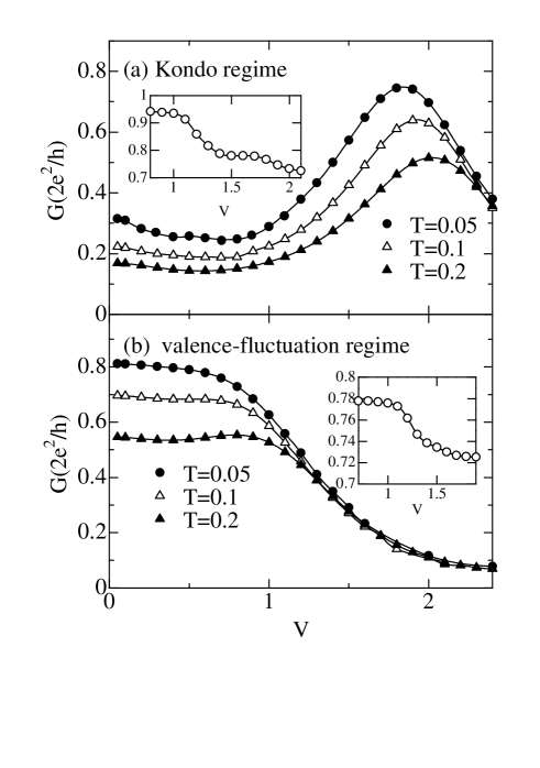
Fig.  2: Conductance for the T-shaped double-dots system as a function of the inter-dot coupling $V$ at various temperatures: (a) Kondo regime with the bare energy levels $\epsilon_{l}=-2.0$ and $\epsilon_{r}=-3.0$, (b) valence-fluctuation regime with $\epsilon_{l}=-1.0$ and $\epsilon_{r}=-2.0$. The inset shows the conductance computed by the SBMF approximation at zero temperature. In the Kondo regime (a), the electron number occupying the left (right) dot is $n_{l}\simeq 1.0$ ($n_{r}\simeq 1.0$) for $V=0.1$, and $n_{l}\simeq 1.0$ ($n_{r}\simeq 0.9$) for $V=1.5$. On the other hand, in the valence fluctuation regime (b), $n_{l}\simeq 0.6$ ($n_{r}\simeq 1.0$) for $V=0.1$, and $n_{l}\simeq 0.5$ ($n_{r}\simeq 0.5$) for $V=1.5$.

We start with the Kondo regime shown in Fig. 2(a). It is seen that the conductance is gradually enhanced with the decrease of the temperature almost in the whole range of $V$ shown in the figure. For small $V$, the enhancement is clearly attributed to the Kondo effect due to the left dot, which is indeed confirmed from the DOS shown in Fig. 3. Namely, for small inter-dot coupling ($V=0.1$), it is seen that the left dot has the typical DOS expected for a single-dot Kondo system, while the right dot has a sharp delta-function type spectrum similarly to an isolated dot. When the inter-dot coupling becomes large, the left- and right-dot levels are mixed up considerably, leading to the upper and lower levels given by

$$\epsilon_{\pm}=\frac{1}{2}\left[(\epsilon_{l\sigma}+\epsilon_{\epsilon_{r\sigma}})\pm\sqrt{(\epsilon_{l\sigma}-\epsilon_{\epsilon_{r\sigma}})+4V^{2}}\right].$$ (17)

The effective upper level is pushed upward with the increase of $V$, resulting in the increase of the conductance. It should be noted that the conductance strongly depends on the temperature even when the effective upper level is located around the Fermi level. Its temperature dependence is not due to the Kondo effect, but is mainly caused by that of the Coulomb peak itself, as seen in the corresponding DOS for the intermediate inter-dot coupling $V=1.0$ in Fig. 3. This implies that the electron correlations play a crucial role for the conductance even in this parameter regime. As the inter-dot tunneling further increases, the upper level goes beyond the Fermi energy. It is remarkable that a tiny resonance peak again appears around the Fermi level. This peak is identified with the Kondo resonance because it gradually develops with the decrease of the temperature, as seen in the inset of Fig. 3(a). However, the resulting Kondo temperature is rather small, and the conductance via the Kondo resonance is hindered by that caused by the upper level. Therefore in the parameter regime $V\sim 2.4$, the conductance is not so much enhanced with the decrease of the temperature, although the small Kondo peak indeed exists.

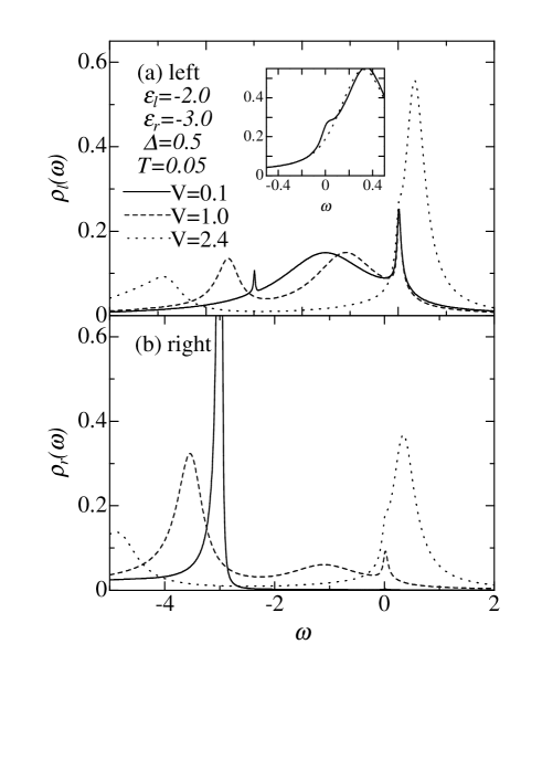
Fig.  3: Local density of states in the Kondo regime at $T=0.05$: (a) left dot, (b) right dot. The solid, dashed and dotted lines correspond to the results for $V=0.1$, $V=1.0$ and $V=2.4$ respectively. The inset in (a) shows $\rho_{l}(\omega)$ for $V=2.4$, where the solid line is for $T=0.05$ and the dotted line for $T=0.2$. The effective Kondo temperature is about 0.01 for $V=0$. The Fermi level is taken to be $\omega=0$.

As mentioned before, our NCA results become less reliable at low temperatures. To overcome this problem, we calculate the conductance by the SBMF theory at zero temperature. The results are shown in the inset of Fig. 2 (a). It is seen that for small $V$ ($\sim 0.1$), the conductance is increased almost up to the unitary limit, while in the intermediate regime $V\sim 2$, the conductance is not so much enhanced. In the strong $V$ regime, the conductance is enhanced, but the effective Kondo peak is shifted slightly away from the Fermi level, so it does not reach the unitary limit. In this way, the SBMF results confirm that the conductance calculated by the NCA approach indeed gives reliable results.

We next discuss the valence-fluctuation regime. The calculated conductance is shown in Fig. 2 (b), and the corresponding DOS is shown in Fig. 4. As mentioned above, when the inter-dot tunneling $V$ increases, two dot levels are separated and thus the upper (lower) level is shifted beyond (below) the Fermi level. Therefore, the conductance is decreased since the Coulomb peak disappears around the Fermi level. This is indeed seen in the finite-temperature NCA results as well as the zero-temperature SBMF results in Fig. 2(b). As mentioned in the case of the Kondo regime, in the large $V$ regime, a tiny Kondo peak appears, which can be also seen in the DOS in Fig. 4.

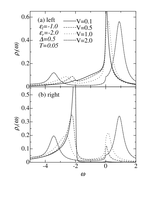
Fig.  4: Local density of states in the valence-fluctuation regime at $T=0.05$: (a) left dot, (b) right dot. The solid, dashed, dotted and dot-dashed lines correspond to $V=0.1$, $V=0.5$, $V=1.0$ and $V=2.0$ respectively. The Fermi level is taken to be $\omega=0$.

3.2 Tuning the dot-levels

We now investigate how the conductance is changed when the energy level of the left or right dot is tuned. This may be experimentally studied by changing the gate voltage.

3.2.1 Conductance control by the left dot

We start by examining the conductance as a function of the left-dot level, $\epsilon_{l}$. The results are shown in Fig. 5.

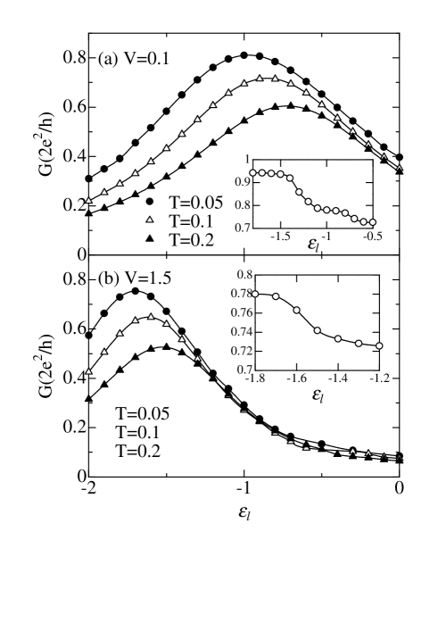
Fig.  5: Conductance for the T-shaped double-dots system as a function of the left-dot level $\epsilon_{l}$ with $\epsilon_{r}=-3.0$ being fixed: (a) $V=0.1$ and (b) $V=1.5$.

Most of the characteristic properties in this case can be understood from the discussions given in the previous subsection. In the weak inter-dot coupling regime shown in Fig. 5 (a), the conductance is enhanced due to the formation of the Kondo resonance as the temperature decreases when $\epsilon_{l}$ is sufficiently deep. As $\epsilon_{l}$ approaches the Fermi level, the conductance is dominated by the current via the bare resonance formed around the effective energy level of the left dot. This type of the interpretation is also valid for the strong inter-dot coupling regime shown in Fig. 5 (b), for which the effective level should be replaced by the resultant upper level, $\epsilon_{+}$. In this case, the temperature dependence of the conductance is understood by the same reason mentioned in Fig. 2 (b). We note that the Kondo peak appears again even for $\epsilon_{l}\sim 0$, but the conductance is mainly dominated by the resonance of the upper level existing near the Kondo peak.

3.2.2 Conductance control by the right dot

We finally discuss the conductance by tuning the energy level of the right dot, $\epsilon_{r}$. We again investigate two cases with small and large inter-dot coupling $V$. The results are summarized in Fig. 6. Let us start with the case of small $V$. When $\epsilon_{r}$ of the right dot is deep below $\epsilon_{l}$, the conductance is mainly controlled by the Kondo mechanism of the left dot, as already mentioned before. This is also valid for the case when $\epsilon_{r}$ is higher beyond $\epsilon_{l}$. These effects are indeed seen in the conductance of Fig. 6(a). Namely we can see the Kondo enhancement of conductance with the decrease of the temperature.

It should be remarked that we encounter a novel interference phenomenon, i.e. nontrivial suppression of the conductance, when two bare dot-levels coincide with each other. This is observed both in the NCA results as well as the SBMF results in Fig. 6(a) around $\epsilon_{r}\sim-2.0$. This may be regarded as a Fano-like effect caused by the interference between two distinct channels,${}^{\hbox{\immediate{?},\penalty 1000\hskip 0.91003pt plus 0.70004pt minus 0.70004pt{?},\penalty 1000\hskip 0.91003pt plus 0.70004pt minus 0.70004pt{?})}}$ i.e. the direct Kondo resonance of the left dot and the indirect resonance via both of the right and left dots. As $V$ becomes large, such interference is smeared, and cannot be observed in Fig. 6(b). We wish to mention that this type of dip structure can be also seen in Fig. 5(a) if the left level is varied through the point $\epsilon_{l}\sim\epsilon_{r}=-3.0$.

In order to clarify the origin of the interference effect, we observe how the DOS changes its character when the right dot level is changed with $V=0.1$ being fixed. It is seen in Fig.7 that when two localized levels are separated energetically, the DOS of the left dot is analogous to that for the ordinary single-dot Anderson model, which is slightly modified around $\epsilon_{r}$ by the hybridization effect of the right dot. Therefore, in this parameter regime, the conductance is mainly controlled by the Kondo resonance of the left dot. However, when two levels are almost degenerate ($\epsilon_{r}=\epsilon_{l}=-2.0$), the left and right states are equally mixed together to lift the degeneracy, and make two copies of similar DOS. As a consequence, this change around the bare levels indirectly modifies the Kondo resonance, namely, it supresses the formation of the Kondo peak around the Fermi level, as seen from Fig.7 for $\epsilon_{r}=-2.0$. This thus gives rise to the decreace in the conductance. It is to be noted here that such an interference effect occurs when the right level is changed in the energy range of the order of $\Delta$, while the relevant temperature range, in which such an effect may be observable, is given by the effective Kondo temperature. Therefore, both of the bare and renormalized (Kondo) energy scales play a crucial role in this interference phenomenon.

It is instructive to point out that the interplay of the Kondo effect and the interference effect appears for smaller $V$, which may be suitable for this effect to be observed in experiments.

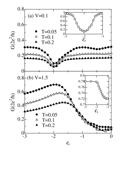
Fig.  6: Conductance for the T-shaped double-dots system as a function of the right-dot level $\epsilon_{r}$ with $\epsilon_{l}=-2.0$ being fixed: (a) $V=0.1$ and (b) $V=1.5$.

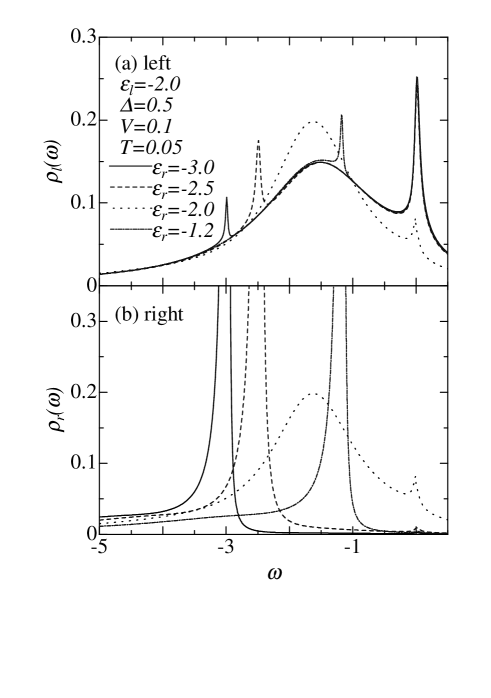
Fig.  7: Local density of states for $V=0.1$. The energy level $\epsilon_{r}$ of the right dot is systematically changed with a

4 Summary

We have studied electron transport in the T-shaped double-dots system as a function of the inter-dot coupling as well as the dot levels. We have calculated the tunneling conductance by exploiting the NCA at finite temperatures as well as the SBMF treatment at zero temperature. It has been found that though the electron current flows only through the left dot, its behavior is considerably affected by the additional right dot via the interference effect. This demonstrates that the transport properties of the system may be controlled by properly tuning the parameters of the right dot which is indirectly connected to the leads.

In particular, we have found a remarkable interference phenomenon for a small inter-dot coupling in the Kondo regime; the conductance is suppressed when two bare dot-levels coincide with each other energetically, which is caused by the interference effect between two distinct channels mediated by the left and right dots. This effect may be observed experimentally around or below the Kondo temperature by appropriately tuning the gate voltage for the dots in the range of the resonance energy due to the inter-dot coupling. In real double-dots systems, the inter-dot tunneling may be rather small, which may provide suitable conditions for our proposed phenomenon to be observed.

References

- [1] L.I. Glazman and M.E. Raikh: JETP Lett: 47 (1988) 452
- [2] Y. Meir, N.S. Wingreen and P. A. Lee: Phys. Rev. Lett. 66 (1991) 3048
- [3] N.S. Wingreen and Y. Meir: Phys. Rev. B 49 (1994) 11040
- [4] A. Kawabata: J. Phys Soc. Jpn 60 (1991) 3222
- [5] A. Oguri, H. Ishii and T. Saso: Phys. Rev. B 51 (1995) 4715
- [6] D. Goldhaber-Gordon, J. Gres, M. A. Kastner, Hadas Shtrikman, D. Mahalu, and U. Meirav: Phys. Rev. Lett. 81 (1998) 5225
- [7] S.M. Cronenwett, T.H. Oosterkamp and L.P. Kouwenhoven: Science 281 (1998) 540
- [8] J. Schmid, J. Weis, Keberl and K.v.Klizing: Physica B 256 (1998) 182
- [9] F. Simmel, R.H. Blick, J.P. Kotthaus, W. Wegscheider and M. Bicher: Phys. Rev. Lett. 83 (1999) 804
- [10] S. Tarucha, D.G. Austing, T. Honda, R.J. van der Hage and L.P. Kouwenhoven: Phys. Rev. Lett. 77 (1996) 3613
- [11] D.G. Austing, T. Honda and S. Tarucha: Jpn. J. Appl. Phys., Part 1 36 (1997) 1667
- [12] F.R. Waugh, M.J Mar, R.M. Westervelt, K.L. Campman and A.C. Gossard: Phys. Rev. Lett. 75 (1995) 705
- [13] R.H. Blick, D. Pfannkuchke, R.J. Haug, K.v. Klitzing and K. Eberl: Phys. Rev. Lett. 80 (1998) 4032
- [14] T.H. Oosterkamp, T. Fujisawa, W.G. van der Wiel, K. Ishibashi, R.V. Hijman, S. Tarucha and L.P. Kouwenhoven: Nature (London). 395 (1998) 873
- [15] T.Aono, M. Eto and K. Kawamura: J. Phys. Soc. Jpn 67 (1998) 1860
- [16] T. Aono and M. Eto: Phys. Rev. B 63 (2001) 125327
- [17] O. Sakai, Y.Shimizu and T. Kasuya: Solid State Commun. 75 (1990) 81
- [18] W. Izumida and O. Sakai: Phys. Rev. B 62 (2000) 10260
- [19] W. Hofstetter and H. Scheller: Phys. Rev. Lett. 88 (2002) 016803
- [20] M. Vojta, R. Bulla and W. Hofstetter: cond-mat/0106458
- [21] U. Fano: Phys. Rev. 124 (1961) 1866
- [22] B. R. Bulka and P. Stefaski: Phys. Rev. Lett. 86 (2001) 5128
- [23] W. Hofstetter J. Knig and H. Scheller: Phys. Rev. Lett. 87 (2001) 156803
- [24] J. Gres, D. Goldhaber-Gordon, S. Heemeyer, and M. A. Kastner: Phys. Rev. B 62 (2000) 2188
- [25] P. Coleman: Phys. Rev. B 29 (1983) 3035
- [26] Y. Kuramoto: Z. Phys. B 53 (1983) 37
- [27] N. E. Bickers: Rev. Mod. Phys. 59 (1987) 845
- [28] Th. Pruschke and N. Grewe: Z. Phys. B 74 (1989) 439
- [29] Y. Imai and N. Kawakami: J. Phys. Soc. Jpn 70 (2001) 1851
- [30] B.A. Jones, G. Kotoliar and A.J. Millis: Phys. Rev. B 39 (1989) 3415
- [31] A.C. Hewson, The Kondo Problem to Heavy Fermions (Cambridge University Press, Cambridge) 1993
- [32] Y.Meir, N.S. Wingreen and P.A. Lee, Phys. Rev.Lett. 70 (1993) 2601