Universality in escape from a modulated potential well

Abstract

We show that the rate of activated escape $W$ from a periodically modulated potential displays scaling behavior versus modulation amplitude $A$. For adiabatic modulation of an optically trapped Brownian particle, measurements yield $\ln W\propto(A_{\rm c}-A)^{\mu}$ with $\mu=1.5$. The theory gives $\mu=3/2$ in the adiabatic limit and predicts a crossover to $\mu=2$ scaling as $A$ approaches the bifurcation point where the metastable state disappears.

Activated processes, such as escape from a metastable state, are exponentially sensitive to time-dependent external perturbations. Escape in driven systems has been investigated in studies of Josephson junctions Larkin ; Devoret and infrared photoemission photoemission . It has been also explored recently in the context of thermally activated magnetization reversal in nanomagnets driven by a time-dependent magnetic field Wernsdorfer97 or a spin-polarized current Ralph02 . The strong dependence of the rates of activated processes on the wave form of the driving field enables selective control of the rates, which is important for many applications, for example control of rate and direction of diffusion in spatially periodic systems ratchets .

In this paper we investigate the dependence of the rate of activated escape $W$ on the amplitude $A$ of a periodic driving field. We show that this dependence displays universal behavior for large $A$ and investigate the scaling of $\ln W$ with $A$. Experimental results are obtained for a colloidal particle trapped in a modulated optically-generated potential. This system was used earlier McCann-99 for a quantitative test of the Kramers theory Kramers of activated escape over a stationary potential barrier. We observe a power-law behavior of $\ln W$ as $A$ approaches a critical value. The critical exponent for adiabatic modulation is $\mu=1.5$, in agreement with theory. Adiabaticity is always violated close to the bifurcation point, and we predict the emergence of a different scaling, with $\mu=2$.

Field dependence of the escape rate is well understood for adiabatically slow modulation, where the field frequency $\omega_{F}$ is small compared to the reciprocal relaxation time $t_{\rm r}^{-1}$. The driven system remains instantaneously in thermal equilibrium. The adiabatic escape rate $W_{\rm ad}\propto\exp[-R_{\rm ad}/k_{B}T]$ depends on the field primarily through the instantaneous activation energy $R_{\rm ad}(t)$. Even where the modulation of $R_{\rm ad}$ is small compared to the zero-field $R_{\rm ad}$, it may still substantially exceed $k_{B}T$, leading to strong modulation of $W_{\rm ad}$.

Finding the escape rate becomes more complicated for nonadiabatic modulation, where $\omega_{F}\gtrsim t_{\rm r}^{-1}$, because a driven system is far from thermal equilibrium. The problem has been addressed theoretically for different models of fluctuating systems Larkin ; Graham-84 ; Dykman-97ab ; SDG ; Hanggi-00 ; M&S-01 . The underlying idea is that activated escape results from an optimal fluctuation, which brings the system from a metastable to an appropriate saddle-type periodic state. We use it here to draw general conclusions about the scaling of the period-averaged escape rate $\bar{W}$ with the field amplitude $A$.

The field dependence of $\ln\bar{W}$ for $\bar{W}\ll t_{\rm r}^{-1},\omega_{F}$ is sketched in Fig. 1. For small $A$, the field is a perturbation. Its major effect is to heat the system, with the change of the effective energy-dependent temperature quadratic in $A$ (the lowest order term after period averaging). As a result, $\ln\left[\bar{W}/W_{0}\right]\propto A^{2}$, where $W_{0}$ is the escape rate in the absence of modulation Larkin ; Devoret . The range of $A$ is limited to $\ln\left[\bar{W}/W_{0}\right]\lesssim 1$.

Figure 1: Amplitude scaling of the period-averaged rate of escape $\bar{W}$ from the modulated potential well shown in the inset ($W_{0}$ is the escape rate in the absence of modulation). The metastable state of forced vibrations disappears once the modulation amplitude reaches the critical value ${\cal A}_{\rm c}$.

For stronger modulating fields, the activation energy of escape $R\propto\ln\bar{W}$ becomes linear in the amplitude $A$ Dykman-97ab . This behavior occurs because the optimal fluctuation leading to escape is a real-time instanton Langer , with duration $\sim t_{\rm r}$. In the absence of modulation, escape has the same probability to happen at any time. Modulation lifts the time degeneracy and synchronizes escape events. As a result, even for zero-mean modulation $\ln\bar{W}/W_{0}\propto A$. For an overdamped Brownian particle, an explicit solution was obtained SDG throughout the heating and log-linear regions in Fig. 1, and the results have been confirmed by extensive simulations Chaos-01 .

As we show in this paper, there is another region where the dependence of $\bar{W}$ on $A$ is universal and unexpected: the vicinity of the saddle-node bifurcation point ${\cal A}_{\rm c}$ where the metastable state of forced vibrations merges with a saddle-type periodic state Guckenheimer . In this range one of the motions of the system becomes slow. The universality is related to the corresponding critical slowing down. However, it turns out that the system can display different types of critical behavior depending on the relationship between $\omega_{F}$ and the relaxation time in the absence of driving $t_{{\rm r}0}$.

Experiments on amplitude-dependent escape from a sinusoidally modulated potential were performed using an optically-trapped Brownian particle in water. A configurable optical potential was constructed by focusing two parallel laser beams through a single microscope objective lens. Each beam creates a stable three-dimensional trap as a result of electric field gradient forces exerted on a transparent dielectric spherical silica particle of diameter 0.6 $\mu$m. At the focal plane, the beams are typically displaced by 0.25 to 0.45 $\mu$m, creating a double-well potential. The depths of the potential wells and the height of the intervening barrier, which is typically 1 to 10 $k_{B}T$, are readily controlled by adjusting beam intensities and separations.

The two HeNe lasers (17 mW, 633 nm) that create the traps are stabilized by electro-optic modulators and imaged into a sample cell by a 100x objective. The beams are mutually incoherent and circularly polarized when they enter the microscope. A single trapped colloidal sphere is imaged onto a digital camera operating at 200 frames/s. The $x$ and $y$ coordinates of the sphere’s center are computed using a pattern matching routine that yields spatial resolution better than 10 nm, whereas the $z$ coordinate parallel to the light wave vector is extracted by analysis of the image as the particle position fluctuates about the focal plane. The overall analysis and storing of the sphere’s $(x,y,z)$ coordinates is accomplished in less than a frame duration so that no images need to be recorded.

The stability of the system is sufficient to compute the full 3-dimensional optical potential from long-time measurements of the particle probability density McCann-99 . The absolute transition rates calculated from the Kramers expression using measured curvatures at the stable and unstable points of the potential are in quantitative agreement with the experimental data over 4 orders of magnitude.

The electro-optic modulators that stabilize the optical traps also enable ac modulation with arbitrary waveforms derived from an electronic signal generator. When the two beams overlap at the separations required to form a potential barrier in the range 5 to 8 $k_{B}T$, each contributes to the position and shape of both potential minima and the potential in the intermediate range. As a consequence of this nonlocality, a small modulation of one beam causes a nearly antisymmetric change of both barrier heights.

The results on over-barrier transitions from one of the wells for the modulating signal $F(t)=A\cos\omega_{F}t$ are plotted in Fig. 2. The amplitude $A$ in Fig. 2 is normalized to $k_{B}T$, where T = 298 K. The intrawell relaxation rate in the absence of modulation $t_{{\rm r}0}^{-1}\approx 10^{3}$ s^-1 McCann-99 is much larger than $\omega_{F}$, so the data fall into the adiabatic regime. In this case escape is most likely to occur when the instantaneous potential barrier $\Delta U(t)$ is minimal. For large modulation amplitude and for temperatures used here, the maximal escape rate $W_{m}$ becomes comparable to the modulation frequency, and therefore it is $W_{m}$ rather than the period-averaged rate $\bar{W}$, that is the more relevant measure. In obtaining $W_{m}$ we used the distribution of the dwell time illustrated in the inset to Fig. 2. The dwell time was computed for the modulated double-well system as the time interval between the appearance in, and escape from, a well.

The solid line in Fig. 2 represents a least-squares fit to the data for large $A$ using the function $\ln W_{m}/W_{0}=C_{1}-C_{2}(A_{\rm c}-A)^{\mu}$, where $\mu=1.5$, and the critical modulation amplitude $A_{\rm c}$ and $C_{1,2}$ are fitting parameters uncertainties .

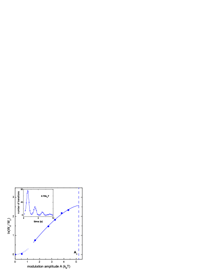
Figure 2: Modulation amplitude dependence of the maximal transition rate $W_{m}$ normalized to $W_{0}$, the unmodulated transition rate. The data points represent the transition rates for an unmodulated barrier $\Delta U_{0}/k_{B}T=5.8$ ($W_{0}=0.069$ s^-1). The solid line is a least-squares fit to the data with an asymptotic form described by the theory (see text). The modulation frequency $\omega_{F}/2\pi=0.4$ Hz. Inset: the number of transitions for $A=2.75k_{B}T$ versus time.

To interpret these results we will consider activated escape in the system for $A$ close to the critical amplitude ${\cal A}_{\rm c}$ where the metastable and unstable periodic states merge. In the adiabatic approximation, the stable and unstable states correspond to the potential well and the barrier top. Once per period, when the driving $|F(t)|$ is a maximum (for example when $t=n\tau_{F},\,n=0,\pm 1,\ldots$), the stable and unstable states are closest to each other and the barrier height $\Delta U(t)$ is a minimum. We take $F(0)$ positive, $F(0)=A$. The well and barrier top merge for $A=A_{\rm c}$, which is the adiabatic bifurcation point.

For small $\delta A=A-A_{\rm c}$ and $|t-n\tau_{F}|$, the dynamics of the system near the metastable state is slow Guckenheimer . It is described by the “soft mode” with coordinate $q(t)$. For negative $\delta A$ the system has a stable and an unstable state, $q_{a}$ and $q_{b}$. We set $q=0$ at the saddle-node state where they merge in the limit of small $\omega_{F}$ for $A=A_{\rm c},t=n\tau_{F}$. Close to $A_{\rm c}$ and $n\tau_{F}$ the equation of motion for $q$, neglecting fluctuations, takes the form

$$t_{{\rm r}0}{dq\over dt}=q^{2}+F(t)-A_{\rm c}$$ (1)

($t_{{\rm r}0}$ is the relaxation time for $F=0$, $\omega_{F}t_{{\rm r}0}\ll 1$). In the adiabatic approximation, $F(t)$ depends parametrically on $t$. Activated transitions occur over the instantaneous barrier $\Delta U(t)=(4/3)[A_{\rm c}-F(t)]^{3/2}$.

The relaxation time of the system $t_{\rm r}=t_{{\rm r}0}[A_{\rm c}-F(t)]^{-1/2}$ becomes large close to the bifurcation point. Therefore even a slowly varying field will ultimately become too fast for the system to follow adiabatically. To allow for nonadiabaticity we expand $F(t)$ in the region of small $\omega_{F}|t-n\tau_{F}|$. The equation of motion (1) in scaled variables $Q=q/\Omega,\;\tau=\Omega(t-n\tau_{F})/t_{{\rm r}0}$ is then

$$\dot{Q}=K(Q,\tau),\;K=Q^{2}+\zeta-\tau^{2},\;$$ (2)

with $\zeta=\Omega^{-2}(A-A_{\rm c})$. In Eq. (2) $\dot{Q}\equiv dQ/d\tau$, and $\Omega=(-{1\over 2}t_{{\rm r}0}^{2}d^{2}F/dt^{2})^{1/4}$ (the derivative is evaluated at $t=0$ and $A=A_{\rm c}$). For sinusoidal modulation $\Omega=(A_{\rm c}t_{{\rm r}0}^{2}\omega_{F}^{2}/2)^{1/4}$.

The dynamics (2) is determined by one dimensionless parameter $\zeta$. For $-\zeta\gg 1$, the adiabatic approximation applies, and the stable and unstable states are given by $Q_{a,b}(\tau)=\mp(-\zeta+\tau^{2})^{1/2}$. On the other hand, for $|\zeta|\lesssim 1$ the time dependence of the states becomes distorted and asymmetric, cf. inset in Fig. 3. For $\zeta=1$, the states given by Eq. (2) merge and $Q_{a}(\tau)=Q_{b}(\tau)=\tau$. The corresponding nonadiabatic bifurcational value of the amplitude is $A_{\rm b}=A_{\rm c}+\Omega^{2}$.

Figure 3: The scaled activation energy of escape $S\approx-\tilde{D}\ln W_{t}$ (dots), obtained numerically from the variational problem (3), vs. $\zeta=\Omega^{-2}(A-A_{\rm c})$. In the adiabatic approximation $S={4\over 3}(-\zeta)^{3/2}$ (the dashed line), which explains the results in Fig. 2. The nonadiabatic bifurcation point is $\zeta=1$. The solid lines show the corrected adiabatic expression for large-$|\zeta|$, Eq. (4), and the nonadiabatic behavior $S\propto(1-\zeta)^{2}$, Eq. (5). Inset: the attracting and repelling states $Q_{a}$ and $Q_{b}$ (thin lines) for weakly nonadiabatic driving, Eq. (2) with $\zeta=0.95$, and the most probable escape path (thick line).

Escape from the attractor can be quite generally described by adding a random Gaussian force to Eq. (1). Because the system dynamics is slow, this force is effectively $\delta$-correlated (white noise), with intensity $D\propto k_{B}T$ for thermal noise. The corresponding force $\xi(\tau)$ in Eq. (2) for $\dot{Q}$ has a correlator $\langle\xi(\tau)\xi(\tau^{\prime})\rangle=2\tilde{D}\delta(\tau-\tau^{\prime}),\;\tilde{D}=D/\Omega^{3}t_{{\rm r}0}.$

The noise-driven system is most likely to escape during the time when $F(t)$ is close to its maximum. The total probability to escape over this time is $W_{t}=\bar{W}\tau_{F}$, where $\bar{W}$ is the period-averaged escape rate. We will calculate $W_{t}$ assuming that the noise intensity $D$ is the smallest parameter of the theory, in which case $W_{t}\propto\exp(-R/D)$. The calculation can be done by generalizing the instanton technique Chaos-01 to the Langevin equation $\dot{Q}=K(Q,\tau)+\xi(\tau)$. The activation energy of escape $R=(D/\tilde{D})S$ is given by the solution of the variational problem

$$S={1\over 4}\min\int\nolimits_{-\infty}^{\infty}d\tau(\dot{Q}-K)^{2}.$$ (3)

The boundary conditions are $Q(\tau)\to Q_{a}(\tau)$ for $\tau\to-\infty$ and $Q(\tau)\to Q_{b}(\tau)$ for $\tau\to\infty$. They correspond to the picture in which, prior to escape, the system is performing small fluctuations about the metastable state $Q_{a}$. Escape occurs as a result of a large fluctuation that brings the system to the saddle state $Q_{b}$. The most probable among such fluctuations is the one in which the system moves along a trajectory [the most probable escape path (MPEP)] that minimizes the functional (3). From Eq. (3), the activation energy $R$ is a function of one parameter $\zeta$, shown in Fig. 3.

An explicit expression for $R$ can be obtained in the adiabatic limit $-\zeta\gg 1$. Here, one can ignore the term $\tau^{2}$ in $K$ (2) for typical $|\tau|\lesssim\zeta^{-1/2}$. Then the MPEP is an instanton $Q_{\rm opt}(\tau,\tau_{0})=|\zeta|^{1/2}\tanh\left[|\zeta|^{1/2}(\tau-\tau_{0})\right]$ centered at an arbitrary $\tau_{0}$. The adiabatic activation energy is $R\propto S=(4/3)(-\zeta)^{3/2}\propto(A_{\rm c}-A)^{3/2}$ 3/2 . This agrees with the experimental data shown in Fig. 2.

The time-dependent term in $K$ lifts translational invariance of the instanton $Q_{\rm opt}(\tau,\tau_{0})$ and synchronizes escape events. The action $S$ is minimal for $\tau_{0}=0$. To lowest order in $1/\zeta$

$$S\approx(4/3)|\zeta|^{3/2}+(\pi^{2}/6)|\zeta|^{-1/2}.$$ (4)

From (4), the nonadiabatic correction to the activation energy diverges as $|\delta A|^{-1/2}$ as $A$ approaches $A_{\rm c}$.

The activation energy may also be found explicitly close to the bifurcation point $\zeta=1$. In this case escape is most likely to occur while the coexisting attracting and repelling trajectories $Q_{a}(\tau)$ and $Q_{b}(\tau)$ stay close to each other. Because of the special structure of the states $Q_{a,b}(\tau)$, the variational problem (3) for the MPEP can be linearized and solved, giving

$$S=(\pi/8)^{1/2}(1-\zeta)^{2},\;1-\zeta\ll 1.$$ (5)

Eq. (5) shows that, near the nonadiabatic bifurcation point $A_{\rm b}$, there emerges another scaling region, where the activation energy $R\propto(A_{\rm b}-A)^{2}$. The nonadiabatic exponent is thus $\mu=2$, in contrast to $\mu=3/2$ in the adiabatic limit. It describes $R(A)$ for the modulation amplitude lying between $A_{\rm c}$ and $A_{\rm b}$, as seen from Fig. 3. The width of this interval is $\propto\omega_{F}$ provided $\omega_{F}t_{{\rm r}0}\ll 1$.

The above theory does not apply in the exponentially narrow range $1-\zeta\lesssim\exp[-C/\omega_{F}t_{{\rm r}0}]$ ($C\sim 1$). This is because, as $A$ approaches $A_{\rm b}$, the relaxation time of the system $t_{\rm r}$ becomes logarithmically long. Then the expansion of the driving force in $t/\tau_{F}$ that leads to the equation of motion (2) becomes inapplicable. For $\omega_{F}t_{\rm r}\gg 1$ the duration of the MPEP greatly exceeds the period $\tau_{F}$. In this case the activation energy again displays the $\mu=3/2$ power-law dependence on the distance to the true bifurcation value of the amplitude ${\cal A}_{\rm c}$. The $({\cal A}_{\rm c}-A)^{3/2}$-law also applies asymptotically if the driving is nonadiabatic for small $A$.

The experimental data discussed above refer to very small $\omega_{F}t_{{\rm r}0}<10^{-3}$. Therefore the nonadiabatic region of modulating amplitudes is narrow and the activation energy there is less than $k_{B}T$. Higher modulation frequencies will be required to detect the crossover from the observed $\mu=3/2$ scaling to the nonadiabatic $\mu=2$ scaling. It appears that the $\mu=3/2$ scaling function describes the data in a broad range of $A$. It thus provides a good interpolation of the activation energy from the linear in $A$ to the critical region.

In conclusion, we have identified several regions where the activation energy $R$ of escape from a metastable potential displays scaling behavior as a function of the amplitude $A$ of an externally applied periodic modulation. We have demonstrated with a system whose potential was directly measured that, near the amplitude $A_{\rm c}$ where the local minimum and maximum of the potential contact one another, $R\propto(A_{\rm c}-A)^{3/2}$. We have also shown that, because of nonadiabaticity near the bifurcation point, there necessarily emerges a region where the scaling exponent changes from $\mu=3/2$ to $\mu=2$. We expect that these scalings can be observed in other systems, such as modulated Josephson junctions Devoret and nanomagnets Wernsdorfer97 ; Ralph02 ; Koch00 . The ideas discussed here can be used to gain additional insight into the physics of these systems and more generally, activated effects in nonequilibrium systems.

This research was supported by the NSF DMR-9971537 and NSF PHY-0071059.

References

- (1) Present address: Department of Physics, University of Wisconsin-River Falls, River Falls, WI 54022
- (2) A.I. Larkin and Yu.N. Ovchinnikov, J. Low Temp. Phys. 63, 317 (1986); B.I. Ivlev and V.I. Mel’nikov, Phys. Lett. A 116, 427 (1986); S. Linkwitz and H. Grabert, Phys. Rev. B 44 11888, 11901 (1991).
- (3) M.H. Devoret et al., Phys. Rev. B 36, 58 (1987); E. Turlot et al., Chem. Phys. 235, 47 (1998).
- (4) F. Pisani et al., Phys. Rev. Lett. 87, 187403(4) (2001).
- (5) W. Wernsdorfer et al., Phys. Rev. Lett. 78, 1791 (1997); W. Wernsdorfer et al., ibid. 79, 4014 (1997).
- (6) E. B. Myers et al., cond-mat/0203487.
- (7) F. Jülicher, A. Ajdari, and J. Prost, Rev. Mod. Phys. 69, 1269 (1997);
- (8) L.I. McCann, M.I. Dykman, and B. Golding, Nature 402, 785 (1999).
- (9) H. Kramers, Physica (Utrecht) 7, 240 (1940).
- (10) R. Graham and T. Tél, Phys. Rev. Lett. 52, 9 (1984); Phys. Rev. A 31, 1109 (1985).
- (11) V.N. Smelyanskiy et al., Phys. Rev. Lett. 79, 3113 (1997); M.I. Dykman and B. Golding, Fluct. Noise Lett. 1, C1 (2001).
- (12) V.N. Smelyanskiy, M.I. Dykman, and B. Golding, Phys. Rev. Lett. 82, 3193 (1999).
- (13) J. Lehman, P. Riemann, and P. Hänggi, Phys. Rev. Lett. 84, 1639 (2000); Phys. Rev. E 62, 6282 (2000).
- (14) R.S. Maier and D.L. Stein, Phys. Rev. Lett. 86, 3942 (2001).
- (15) J.S. Langer, Ann. Phys. 41, 108 (1967).
- (16) M.I. Dykman, B. Golding, L.I. McCann, V.N. Smelyanskiy, D.G. Luchinsky, R. Mannella, and P.V.E. McClintock, Chaos 11, 587 (2001) and references therein.
- (17) J. Guckenheimer and P. Holmes, Nonlinear Oscillators, Dynamical Systems and Bifurcations of Vector Fields (Springer-Verlag, NY 1987).
- (18) The results of the least squares fit in Fig. 2 are: . We also allowed the critical exponent to vary with a four-parameter fit, which led to the uncertainty .
- (19) For a metastable state near a termination point, is the mean-field exponent describing the vanishing of the free-energy barrier as a termination point is approached along the approriate variable. For (quasi)stationary systems, it was discussed in various contexts, such as Josephson junctions [J. Kurkijärvi, Phys. Rev. B 6, 832 (1972)] and magnets [R.H. Victora, Phys. Rev. Lett. 63, 457 (1989)], as well as fluctuating dynamical systems [M.I. Dykman and M.A. Krivoglaz, Physica A 104, 480 (1980); R. Graham and T. Tél, Phys. Rev. A 35, 1328 (1987)].
- (20) R.H. Koch et al., Phys. Rev. Lett. 84, 5419 (2000).