A Coulomb gas approach to the anisotropic one-dimensional Kondo lattice model at arbitrary filling

Abstract

We establish a mapping of a general spin-fermion system in one dimension into a classical generalized Coulomb gas. This mapping allows a renormalization group treatment of the anisotropic Kondo chain both at and away from half-filling. We find that the phase diagram contains regions of paramagnetism, partial and full ferromagnetic order. We also use the method to analyze the phases of the Ising-Kondo chain.

I Introduction

The relevance of studying the Kondo lattice model (KLM) has not decreased. It is believed to be at the heart of the physics of both the heavy fermion materials, in its antiferromagnetic (AFM) version,Hewson (1997) and also the manganites, when local moments and conduction electrons interact via the ferromagnetic (FM) Hund’s coupling.Dagotto et al. (1998) In the first case, the well understood behavior of the single (or few) impurity Kondo model permeates much of our current understanding. However, the interplay between the local Kondo physics and the non-local RKKY interaction in a lattice environmentDoniach (1977) remains elusive in current approximate schemes, although it may play a prominent role close to quantum critical pointsJ. A. Hertz (1976); A. J. Millis (1993); Coleman et al. (2001); Q. Si et al. (2001) or even away from them. In this respect, a more thorough understanding of the one-dimensional (1D) case might be fruitful, even in light of the peculiarities of 1D systems. Furthermore, the study of the 1D KLM is important in its own right for the analysis of some quasi-one-dimensional organic compounds such as $\rm(Per)_{2}M(mnt)_{2}$ (M=Pt,Pd), bourbonnais ; lopes ; matos and $\rm(DMET)_{2}FeBr_{4}$.enoki

A fairly complete ground state phase diagram has been established for the 1D KLM.Tsunetsugu et al. (1997); Dagotto et al. (1998) On the one hand, the antiferromagnetic model at half-filling has both charge and spin gaps.Tsvelik (1994) For lower band fillings there is a quantum phase transition from a paramagnetic ground state to a ferromagnetic one.Tsunetsugu et al. (1997) On the other hand, the ferromagnetic model at half-filling is also insulating with a Haldane type spin gap.Shibata et al. (1995) For lower band fillings, the numerical evidence shows three distinct phases: a phase with partial ferromagnetic order and incommensurate spin correlations, a fully saturated ferromagnetically ordered phase and a region with phase separation where two kinds of ground state seem to compete. The energy scales where the transitions take place for both models are of the order of the Fermi energy. Finally, there is strong numerical evidence in favor of a Luttinger Liquid behavior in the paramagnetic phase of the AFM KLM, even for considerably large coupling constants.Shibata et al. (1997, 1996); Watanabe (2000) Such phenomenology is beyond a simple RKKY versus Kondo type of picture,Honner and Gulácsi (1998) as proposed by Doniach for the higher dimensional models.Doniach (1977) In fact, the level crossing responsible for the quantum critical point (QCP) is related to long wavelength modes. This is in contrast with the short wavelength spin modes involved in the paramagnetic-antiferromagnetic transition that the Doniach’s picture envisages. As pointed out before,Tsunetsugu et al. (1997); Honner and Gulácsi (1998) the missing element is the lowering of the conduction electron kinetic energy with the alignment of the localized spin as in the double exchange mechanism. Essentially, this is the reason why the 1D FM and AFM KLM have similar phase diagrams.

Despite these successes, it would be considerably more informative if some analytical understanding could be gained. Even though there have been some partial successesZachar et al. (1996); Honner and Gulácsi (1997, 1998); Zachar (2001), there is still room for improvement. Motivated by the enormous success of renormalization group (RG) analyses in the few impurity problem,Anderson and Yuval (1969); Yuval and Anderson (1970); Anderson et al. (1970); Wilson (1975); B. A. Jones et al. (1988) we set out to apply scaling ideas to the 1D lattice case as well. However, an RG treatment of the KLM has never, to our knowledge, been achieved. Technically, although we know how to progressively decimate the spins or the conduction electron states, no one has devised a way of doing both simultaneously, specially with the incorporation of local Kondo physics.

It is the aim of this article to put forth such a decimation scheme for one-dimensional models of spins and fermions, in particular the anisotropic Kondo lattice model. We draw a great deal of inspiration from the original work of Anderson, Yuval and Hamman for the single impurity Kondo model,Anderson and Yuval (1969); Yuval and Anderson (1970); Anderson et al. (1970) mapping the KLM into a classical Coulomb gas, which is then decimated by standard methods.Nienhuis (1987) This task is made simpler by the use of bosonization methods. We therefore study the stability of the non-interacting ground state with respect to the Kondo interaction as a function of the coupling constants. Our study reveals that there is no “weak coupling” flow in the entire parameter space. Nevertheless, the different “strong coupling” flows of the RG equations allow us to assign the magnetic ground states that emerge, establishing the phase diagram for both signs of the coupling constant in a unified fashion. While our approach in part builds upon previous studies,Zachar et al. (1996); Honner and Gulácsi (1997, 1998); Zachar (2001) it also puts on a firmer basis the procedure of neglecting backward scattering terms in the KLM away from half-filling. As another application of our Coulomb gas treatment, we also establish the phase diagram of the one dimensional Ising-Kondo model.Sikkema et al. (1996)

In Section II, we develop a path integral formulation of the bosonized 1D KLM. The partition function is mapped into a two-dimensional generalized classical Coulomb gas in Section III. In Section IV, the RG equations of the Coulomb gas are derived and solved. Their physical interpretation is given in Section V, where an effective Hamiltonian for the renormalized Coulomb gas is obtained. The phase diagram of the model is established in Section VI. The Ising-Kondo model is discussed in Section VII, where its phase diagram is established. We wrap up with a brief discussion of the relation between our and previous results in Section VIII. Some more technical developments can be found in the Appendices.

II Partition Function

We start by writing the 1D KLM Hamiltonian. The traditional Kondo model is isotropic in spin space. Since we are going to use Abelian bosonization, it is natural to break the $SU\left(2\right)$ symmetry down to $U\left(1\right)$

$$H = -t\sum_{j,\sigma}\left(c^{\dagger}_{j+1\sigma}c^{\phantom{\dagger}}_{j\sigma}+h.c.\right)$$ (1)

$$+ J_{\perp}\left(S_{j}^{x}s_{j}^{x}+S_{j}^{y}s_{j}^{y}\right)+J_{z}S^{z}_{j}s^{z}_{j},$$

where $c_{j\sigma}$ destroys a conduction electron in site $j$ with spin projection $\sigma$, $\mathbf{S}_{j}$ is a localized spin $\frac{1}{2}$ operator and $\mathbf{s}_{j}=\frac{1}{2}\sum_{\alpha\beta}c^{\dagger}_{j\alpha}\sigma c^{\phantom{\dagger}}_{j\beta}$, the conduction electron spin density. We will focus on the continuum, long-distance limit of the conduction electrons. In this case, one can linearize the dispersion around the non-interacting $\left(J_{z,\perp}=0\right)$ Fermi points $\pm k_{F}$, where $k_{F}a=\frac{\pi}{2}n$ and $n$ is the conduction electron number density, and take the continuous limit of the fermionic operators in terms of left and right moving field operatorsZachar et al. (1996)

$$H = -iv_{F}\sum_{\sigma}\int dx\left(\psi^{\dagger}_{R,\sigma}\partial_{x}\psi^{\phantom{\dagger}}_{R,\sigma}-\psi^{\dagger}_{L,\sigma}\partial_{x}\psi^{\phantom{\dagger}}_{L,\sigma}\right)$$

$$+ \frac{aJ_{z}}{2}\sum_{j}\sum_{\alpha,\beta,s}\psi_{\alpha,s}^{\dagger}\left(j\right)\psi^{\phantom{\dagger}}_{\beta,s}\left(j\right)\sigma^{z}_{s,s}S^{z}\left(j\right)$$

$$+ \frac{aJ_{\bot}}{2}\sum_{i}\sum_{\alpha,\beta,s,s^{\prime}}\psi_{\alpha,s}^{\dagger}\left(j\right)\psi^{\phantom{\dagger}}_{\beta,s^{\prime}}\left(j\right)\sigma^{\eta}_{s,s^{\prime}}S^{\eta}\left(j\right),$$

where $\alpha,\beta=L\,\,\mathrm{or}\,\,R$, $v_{F}=2t\sin k_{F}a$ is the Fermi velocity and $a$ is the lattice spacing. The field operators can now be bosonized with the inclusion of the so-called Klein factors in usual notationvon Delft and Schoeller (1998)

$$\psi_{R,\sigma}\left(x\right) = \frac{F_{R,\sigma}}{\sqrt{2\pi\alpha}}e^{i\sqrt{\pi}\left[\phi_{\sigma}\left(x\right)-\theta_{\sigma}\left(x\right)\right]+ik_{F}x},$$

$$\psi_{L,\sigma}\left(x\right) = \frac{F_{L,\sigma}}{\sqrt{2\pi\alpha}}e^{-i\sqrt{\pi}\left[\phi_{\sigma}\left(x\right)+\theta_{\sigma}\left(x\right)\right]-ik_{F}x}.$$

One can then rewrite the Hamiltonian in terms of the charge and spin fields

$$\phi_{c,s}\left(x\right) = \left(\phi_{\uparrow}\left(x\right)\pm\phi_{\downarrow}\left(x\right)\right)/\sqrt{2},$$

$$\theta_{c,s}\left(x\right) = \left(\theta_{\uparrow}\left(x\right)\pm\theta_{\downarrow}\left(x\right)\right)/\sqrt{2},$$

as

$$H=H_{0}+H_{z}^{f}+H_{\perp}^{f}+H_{z}^{b}+H_{\perp}^{b},$$ (2)

with:

$$H_{0} = \frac{v_{F}}{2}\sum_{\nu=s,c}\int dx\left(\partial_{x}\phi_{\nu}\right)^{2}+\left(\partial_{x}\theta_{\nu}\right)^{2}$$ (3a)

$$H^{f}_{z} = \sum_{x}\,J^{f}_{z}\sqrt{\frac{2}{\pi}g_{\sigma}}\partial_{x}\phi_{s}\left(x\right)S^{z}\left(x\right)$$ (3b)

$$H^{f}_{\perp} = \sum_{x}\frac{J^{f}_{\perp}}{2\pi\alpha}e^{i\sqrt{\frac{2\pi}{g_{\sigma}}}\theta_{s}\left(x\right)}\cos\left[\sqrt{2\pi g_{\sigma}}\phi_{s}\left(x\right)\right]S^{-}\left(x\right)+h.c.$$ (3c)

$$H^{b}_{z} = \sum_{x}\frac{2J^{b}_{z}}{\pi\alpha}\sin\left[\sqrt{2\pi g_{\rho}}\phi_{c}\left(x\right)+2k_{F}x\right]\sin\left[\sqrt{2\pi g_{\sigma}}\phi_{s}\left(x\right)\right]S^{z}\left(x\right)$$ (3d)

$$H^{b}_{\perp} = \sum_{x}\frac{J^{b}_{\perp}}{2\pi\alpha}e^{i\sqrt{\frac{2\pi}{g_{\sigma}}}\theta_{s}\left(x\right)}\cos\left[\sqrt{2\pi g_{\rho}}\phi_{c}\left(x\right)+2k_{F}x\right]S^{-}\left(x\right)+h.c.$$ (3e)

where $g_{\sigma}=g_{\rho}=1$ and $\alpha\sim k^{-1}_{F}$. $H_{0}$ is the free bosonic Hamiltonian written as a function of $\theta_{s,c}$ and $\phi_{s,c}$. We have introduced the new parameters $g_{\sigma}$ and $g_{\rho}$ for future use. The “relativistic” description enforced by us broke the interaction term in two different components: forward-scattering, $H^{f}$, and back-scattering, $H^{b}$. They involve the spin current and the $2k_{F}$ component of the magnetization of the non-interacting electron gas, respectively,Affleck (1990); Gogolin et al. (1998) since it is well known that the main contributions to the spin susceptibility of the electron gas at low frequencies come from $q\sim 0$ and $q\sim 2k_{F}$. For further generalization, we will consider the 4 parameters $J^{f,b}_{\perp,z}$, as independent.Zachar et al. (1996) It is important to note that the cosines and sines of the bosonic fields in Eqs. (3) are just a short form notation. Forward and backward Klein factors do not have common eigenvectors.Sénéchal (1999) Thus, we shall not neglect their contribution to the simultaneous treatment of $H^{f}$ and $H^{b}$.

A quantum system of dimension $d$ can be mapped into a classical system of dimension $d+1$.Kogut (1979); Baxter (1982) The single impurity Kondo problem has effective dimension $d=0$. The work of Anderson, Yuval, and HammanAnderson and Yuval (1969); Yuval and Anderson (1970); Anderson et al. (1970) showed that it can be mapped into a $d=1$ classical Coulomb gas, where the extra dimension is the imaginary time.Negele and Orland (1988); Gogolin et al. (1998) We will extend this idea and map the 1D KLM into a $d=2$ classical problem. As usual, the starting point is the partition function:

$$Z=Tr\left[e^{-\beta\left(H_{0}+H^{f}+H^{b}\right)}\right].$$ (4)

We will rescale the Hamiltonian and $\beta$ by the Fermi velocity. This introduces the dimensionless coupling constants $\tilde{J}_{z,\bot}=\frac{aJ_{z,\bot}}{v_{F}}$ as well as $\tilde{\beta}=v_{F}\beta$. Following the standard prescription,Fradkin (1991); Negele and Orland (1988) we divide $\tilde{\beta}$ in infinitesimal parts,

$$Z=Tr\left[\prod_{j}e^{-\delta\tau H}\right].$$

In order to proceed to a path integral formulation we choose the $S^{z}$ basis for the local moments and the coherent states for the bosonic fields.Fradkin (1991); Negele and Orland (1988) The next step is to introduce an identity resolution between each exponential in the product

$$Z=\prod_{j}\left\langle\zeta\left(\tau_{j}\right)\right|e^{-\delta\tau H}\left|\zeta\left(\tau_{j}\right)\right\rangle,$$

where we used $\left|\zeta\right\rangle$ to denote a general vector in the basis. We now expand the exponentials in powers of $\delta\tau$,

$$Z=\sum_{n=0}\frac{1}{n!}\left(\delta\tau\right)^{n}\left\langle\zeta\left(j\right)\right|H^{n}\left|\zeta\left(\tau_{j+1}\right)\right\rangle.$$

There are two possible spin configurations for a given pair of consecutive instants along the imaginary time direction:

1. if there is no spin flip between them, the only contributing terms are from the $z$ components of the Hamiltonian (3b) and (3d)

   $$\left\langle\vec{s}\left(x,\tau+\delta\tau\right)\right|S^{z}\left(x\right)\partial_{x}\phi_{s}\left(x\right)\left|\vec{s}\left(x,\tau\right)\right\rangle;$$

   $$\left\langle\vec{s}\left(x,\tau+\delta\tau\right)\right|S^{z}\left(x\right)\sin\left[\sqrt{2\pi g_{\rho}}\phi_{c}\left(x\right)+2k_{F}x\right]$$

   $$\sin\left[\sqrt{2\pi g_{\sigma}}\phi_{s}\left(x\right)\right]\left|\vec{s}\left(x,\tau\right)\right\rangle;$$ (5)

2. if there is a spin flip between these 2 instants, then only (3c) and (3e) contribute

   $$\left\langle\vec{s}\left(x,\tau+\delta\tau\right)\right|e^{i\sqrt{\frac{2\pi}{g_{\sigma}}}\theta_{s}\left(x\right)}\cos\left[\sqrt{2\pi g_{\sigma}}\phi_{s}\left(x\right)\right]$$

   $$S^{-}\left(x\right)+\mathrm{h}.\mathrm{c}.\left|\vec{s}\left(x,\tau\right)\right\rangle;$$

   $$\left\langle\vec{s}\left(x,\tau+\delta\tau\right)\right|e^{i\sqrt{\frac{2\pi}{g_{\sigma}}}\theta_{s}\left(x\right)}\cos\left[\sqrt{2\pi g_{\rho}}\phi_{c}\left(x\right)+2k_{F}x\right]$$

   $$S^{-}\left(x\right)+\mathrm{h}.\mathrm{c}.\left|\vec{s}\left(x,\tau\right)\right\rangle.$$ (6)

The two possible processes above are illustrated in Fig. 1. Several bosonic operators can fit inside the example given in that figure, for example

$$\frac{\tilde{J}^{b}_{z}\tilde{J}^{f}_{\perp}}{2}\left(\sqrt{\frac{2}{\pi}g_{\sigma}}\tilde{J}^{f}_{z}\right)F_{L\uparrow}^{\dagger}F_{R\uparrow}F_{R\downarrow}^{\dagger}F_{R\uparrow}S^{z}\left(x,\tau_{3}\right)S^{+}\left(x,\tau_{2}\right)S^{z}\left(x,\tau_{1}\right)\times$$

$$e^{i\sqrt{2\pi g_{\sigma}}\phi_{s}\left(x,\tau_{3}\right)+i\sqrt{2\pi g_{\rho}}\phi_{c}\left(x,\tau_{3}\right)}e^{i\sqrt{\frac{2\pi}{g_{\rho}}}\theta_{s}\left(x,\tau_{2}\right)-i\sqrt{2\pi g_{\sigma}}\phi_{s}\left(x,\tau_{2}\right)+2ik_{F}x}\partial_{x}\phi_{s}\left(x,\tau_{1}\right),$$

where we regrouped terms to separate Klein factors, local spin operators and bosonic fields.

Figure 1: Example of a spin history. 1 stands for $S_{z}$ operators (Eq. (5)) and $2$ for $S_{\perp}$ones (Eq. (6)).

The lattice parameter in the Euclidean-time direction is set by the bosonic cut-off: $\delta\tau\cong 2\pi\alpha$. Keeping the leading order terms, we write the partition function as the sum over all $d=2$ Ising spin configurations of the localized spins, Klein factors and a functional integral over the bosonic variables. Since there are different types of bosonic exponentials (“vertex operators”), coming from the different interaction terms in Eq. (2), we now introduce new Ising variables which we will call “charges” in order to do the bookkeeping. They give the sign of the corresponding bosonic field in the accompanying exponential according to the following scheme:

1. $m\left(x,\tau\right)=S^{z}\left(x,\tau+\delta\tau\right)-S^{z}\left(x,\tau\right)=\pm 1$ gives the sign of $\theta_{s}\left(x,\tau\right)$ (Eqs. (3c) and (3e))

2. $e\left(x,\tau\right)=\pm 1$ gives the sign of $\phi_{s}\left(x,\tau\right)$ (Eqs. (3c) and (3d))

3. $c\left(x,\tau\right)=\pm 1$ gives the sign of $\phi_{c}\left(x,\tau\right)$ (Eqs. (3d) and (3e))

Note that only $m\left(x,\tau\right)$ is always tied to a localized spin flip process, its value giving both the sign of the $\theta_{s}$ coefficient and the change in $S^{z}$. With this notation, each point in the Euclidean “space-time” is labeled by a triad of values $\left(m,e,c\right)$. We call a “particle” a point where $\left(m,e,c\right)\neq\left(0,0,0\right)$. Each kind of particle matches a certain incident in the history of a spin. From Eqs. 3, we can read off the existence of three breeds of particles, each one with its respective fugacity. Table 1 summarizes the notation that we will use.

fugacity	$\left(m,e,c\right)$	Number of particles
$y_{1}=\tilde{J}^{f}_{\perp}/2$	$\left(\pm 1,\pm 1,0\right)$	$N_{1}$
$y_{2}=\tilde{J}^{b}_{\perp}/2$	$\left(\pm 1,0,\pm 1\right)$	$N_{2}$
$y_{3}=\tilde{J}^{b}_{z}/2$	$\left(0,\pm 1,\pm 1\right)$	$N_{3}$

Table 1: Particles in the 1D KLM and their charges.

Denoting $\eta^{l}_{j}$ as the space-time position of particle $j$ of type $l=\left\{1,2,3\right\}$ and ${\cal D}\eta=\prod^{3}_{l=1}\prod^{N_{l}}_{j=1}d\eta_{j}^{l}$ , we can write the partition function as:

$$Z = \sum_{\left\{\sigma\right\}}\sum_{N_{1},N_{2},N_{3}=0}^{\infty}\sum_{\left\{m,e,c\right\}}\int{\cal D}\phi_{s,c}{\cal D}\theta_{s,c}{\cal D}\eta\,\frac{y_{1}^{N_{1}}y_{2}^{N_{2}}y_{3}^{N_{3}}}{N_{1}!N_{2}!N_{3}!}\,\left(\textrm{Klein factors}\right)\,\left[\prod_{j=1}^{N_{3}}\sigma^{z}\left(\eta_{j}^{3}\right)\right]$$ (7)

$$\exp \left\{-S_{0}-\tilde{J}^{f}_{z}\sqrt{\frac{2}{\pi}g_{\sigma}}\sum_{x}\int d\tau\partial_{x}\phi_{s}\left(x,\tau\right)S^{z}\left(x,\tau\right)+i\sqrt{\frac{2\pi}{g_{\sigma}}}\sum_{l=1,2}\sum_{\eta^{l}_{j}}m\left(\eta^{l}_{j}\right)\theta_{s}\left(\eta_{j}^{l}\right)\right.$$

$$+ \left.i\sqrt{2\pi g_{\sigma}}\sum_{l=1,3}\sum_{\eta^{l}_{j}}e\left(\eta_{j}^{l}\right)\phi_{s}\left(\eta_{j}^{l}\right)+\sqrt{2\pi g_{\rho}}\sum_{l=2,3}\sum_{\eta_{j}^{l}}\left[c\left(\eta_{j}^{l}\right)\phi_{c}\left(\eta_{j}^{l}\right)+2ik_{F}c\left(\eta_{j}^{l}\right)x^{l}_{j}\right]\right\},$$

where $\left\{\sigma\right\}$ stands for all Ising spin configurations, $\left\{m,e,c\right\}$ represents all possible sets of $\sum_{i}N_{i}$ particles, $x^{l}_{j}$ is the space coordinate of particle $\eta^{l}_{j}$ and $S_{0}$ is the free Gaussian bosonic action in the variables $\phi_{s,c}$ and $\theta_{s,c}$Gogolin et al. (1998). There are several restrictions over $\left\{m,e,c\right\}$, usually called neutrality conditions in the bosonizationGogolin et al. (1998) and Coulomb GasNienhuis (1987) literatures. In the 1D KLM they are more stringent than usual, ensuring the compatibility of the sums over $\left\{\sigma\right\}$ and $\left\{m,e,c\right\}$ in Eq (7). Therefore, we will call them strong neutrality conditions (see Appendix A for the derivation of these conditions). They are:

1. for each space coordinate the $m$ charges must be neutral, $\sum_{i}m\left(x_{fixed},\tau_{i}\right)=0$,

2. the total $e$ charge must be neutral, $\sum_{i}e\left(x_{i},\tau_{i}\right)=0$,

3. for each space coordinate the total charge $c$ must be an even integer $\sum_{i}c\left(x_{fixed},\tau_{i}\right)=2n,\,n\in\mathbb{Z}$; and the total charge in the entire space-time must be zero, $\sum_{i}c\left(x_{i},\tau_{i}\right)=0$.

We can immediately see two consequences of these conditions. The most obvious is that the sign of $\tilde{J}^{f,b}_{\perp}$ is irrelevant since, from condition 1, the total number of spin flips in the time direction $N_{1}+N_{2}$ is even. The other consequence is more subtle and more surprising: the complete cancellation of the Klein factors and the product of $\sigma^{z}\left(\eta_{j}^{3}\right)$ in Eq. (7),

$$\left(\textrm{Klein factors}\right)\prod_{j=1}^{N_{3}}\sigma^{z}\left(\eta^{3}_{j}\right)=1.$$

This result plays a central role in the renormalization group treatment of a single Kondo impurity in a LL by Lee and Toner.Lee and Toner (1992) Moreover, it leads to:

$$2k_{F}\sum_{i}c\left(i\right)x_{i}=\left\{\begin{array}[]{l}0,\\ \\ 4k_{F}aI,\,I\in\mathbb{Z}\end{array}\right.,$$ (8)

in each contribution to the partition function. The $2k_{F}$ terms appear whenever there are particles of type $2$ and $3$ (see the definition of the charge $c$ and Eqs. (3d) and (3e)). Due to their oscillatory nature, configurations with these particles will be strongly suppressed in the statistical sum and the corresponding terms (with fugacities $y_{2}=\tilde{J}_{\perp}^{b}/2$ and $y_{3}=\tilde{J}_{z}^{b}/2$) will be irrelevant in the RG sense. This irrelevance criterion is precisely the same as the one used from neglecting Umklapp scattering away from half-filling in models like the Hubbard model.Voit (1995) However, we stress that the situation here is far less trivial than in the Hubbard model, since we have both fermions and spins, and the latter have no independent dynamics, thus hindering a rigorous analysis (an important exception to this is the Heisenberg-Kondo modelSikkema et al. (1997)). In our treatment, on the other hand, spins and fermions are treated on the same footing and lose their independent identity. After the mapping to a Coulomb gas, the irrelevance criterion becomes identical to other models where its applicability is firmly based. We have thus established a more rigorous basis for neglecting the backward scattering terms in the 1D KLM, as has been done by Zachar, Kivelson and Emery.Zachar et al. (1996)

This situation changes when the conduction band is at half filling. In this case, $4k_{F}a=2\pi$ and these terms disappear from the effective action, making all particles equally probable. This commensurability condition is similar to the one for the Umklapp term in the Hubbard model.Voit (1995) It is interesting to note that only the combination $4k_{F}a$ appears in our formulation. Since we bosonized the non-interacting conduction electron sea, we must use $k_{F}a=\pi n/2$, leading to $4k_{F}a=2\pi n$. Even if for some reason a large Fermi surface should be considered,Yamanaka et al. (1997) this would not change any of our results since for a large Fermi surface $4k_{F}^{*}a=2\pi\left(n+1\right)=4k_{F}a\,\mathrm{mod}\,2\pi$.

III Coulomb Gas

The bosonic fields in Eq. (7) can now be integrated out, partially summing the partition function. The result can be understood as an effective action for the spins and the variables $\left(m,e,c\right)$

$$S_{eff} = \left(\frac{\tilde{J}_{z}^{f}}{\pi}\right)^{2}\sum_{x_{1}>x_{2}}\int_{\tau_{1}>\tau_{2}}d\tau_{1}d\tau_{2}\frac{\cos\left(2\varphi_{12}\right)}{r_{12}^{2}}S^{z}\left(1\right)S^{z}\left(2\right)$$ (9)

$$+ \frac{\tilde{J}_{z}^{f}}{\pi}\sum_{n}\sum_{x}\int d\tau\frac{\exp\left(ie\left(n\right)\varphi\right)}{r}S^{z}\left(x,\tau\right)$$

$$+ \sum_{n>p}\frac{\ln z_{np}}{2}\left(m\left(n\right)+e\left(n\right)\right)\left(m\left(p\right)+e\left(p\right)\right)+\frac{\ln\bar{z}_{np}}{2}\left(m\left(n\right)-e\left(n\right)\right)\left(m\left(p\right)-e\left(p\right)\right)$$

$$+ \ln\left|r_{np}\right|c\left(n\right)c\left(p\right)+2ik_{F}\sum_{n}c\left(n\right)x_{l}+\mathrm{short}\,\mathrm{range}\,\mathrm{interactions},$$

where

$$x_{jk} = x_{k}-x_{j},$$

$$\tau_{jk} = \tau_{k}-\tau_{j},$$

$$z_{jk} = x_{jk}+i\tau_{jk}=r_{jk}e^{i\varphi_{jk}}.$$ (10)

In addition to the long range universal interactions, this procedure also gives rise to short-ranged terms that are cutoff dependent.Wiegmann (1978) These are similar to those found by Honner and GulácsiHonner and Gulácsi (1997, 1998) by smoothing the bosonic commutation relations. In contrast to their treatment, though, here they are a manifestation of the bosonic field dynamics. Following Zachar et. al,Zachar et al. (1996) we will focus on the universal long range part of the action and neglect these terms.

Upon integrating by parts in imaginary time, spin time derivatives become the charges we denote by $m$. Finally, we can rewrite all long range terms in the form of a generalized CG action in two-dimensional Euclidean spaceNienhuis (1987) as

$$Z=\sum_{N_{1},N_{2},N_{3}=0}^{\infty}\sum_{\left\{m,e,c\right\}}\int D\eta\frac{y_{1}^{N_{1}}y_{2}^{N_{2}}y_{3}^{N_{3}}}{N_{1}!N_{2}!N_{3}!}\exp\left\{S_{eff}\right\},$$ (11)

with

$$S_{eff} = \frac{1}{2}\sum_{i\neq j}\left\{\frac{\kappa^{2}}{g_{\sigma}}\ln\left|r_{ij}\right|m\left(\eta_{i}\right)m\left(\eta_{j}\right)\right.$$ (12)

$$+ g_{\sigma}\ln\left|r_{ij}\right|e\left(\eta_{i}\right)e\left(\eta_{j}\right)+g_{\rho}\ln\left|r_{ij}\right|c\left(\eta_{i}\right)c\left(\eta_{j}\right)$$

$$- \left.i\kappa\varphi_{ij}\left[e\left(\eta_{i}\right)m\left(\eta_{j}\right)+m\left(\eta_{i}\right)e\left(\eta_{j}\right)\right]\vphantom{\frac{\kappa^{2}}{g_{\sigma}}}\right\}$$

$$+ 2ik_{F}\sum_{i}c\left(\eta_{i}\right)x_{i},$$

where $\kappa=1-\tilde{J}^{f}_{z}/\pi$. In the above effective action we have dropped the superindex indicating the particle type in order to unclutter the notation. It is now unnecessary as the dependence with the history of a spin has disappeared.

In most other similar CG mappings, the coefficient of the term in $\varphi_{ij}$ is an integer and goes by the name of conformal spin.Gogolin et al. (1998) Then, the ambiguity of $2\pi I,\,I\in\mathbb{Z}$ in the angle is irrelevant. In this case, however, $\kappa$ can assume non-integer values. What guarantees that the theory is actually well defined is the strong neutrality condition $1$, which leads to a cancellation of the Riemann surface index $I$.

The integration by parts that we performed is equivalent to applying the duality relation $\partial_{x}\phi_{s}=i\partial_{\tau}\theta_{s}$ to Eq. (7), integrating by parts and then tracing the bosonic fields. Alternatively, at the Hamiltonian level, it is also equivalent to applying the rotationZachar et al. (1996)

$$U=e^{i\sqrt{\frac{2}{\pi}}J^{f}_{z}\sum_{x}\theta_{s}\left(x\right)S^{z}\left(x\right)},$$ (13)

to Eq (2) before going to a path integral and tracing out the bosons. Hence, there is a strong link between our CG formulation and previous results in the literature.Zachar et al. (1996); Honner and Gulácsi (1997, 1998) More importantly, the interpretation of our results should be understood in this rotated basis that mixes spins and bosons.

The effective action in Eq. (12) can be viewed as describing the electrostatic and magnetostatic energy of singly charged particles with both electric and magnetic monopoles. These satisfy electric-magnetic duality in the sense that the action is invariant under the exchange $e\rightleftharpoons m$ and $g_{\sigma}\rightleftharpoons\frac{\kappa^{2}}{g_{\sigma}}$, while $\kappa$ is unchanged. This is analogous to the Dirac relation between electric and magnetic monopoles. Furthermore, these particles possess a third electric-like charge ($c)$, unrelated to the two previous ones. The partition function sum now has been reduced to considering all particle configurations, blending spins and bosons in this Coulomb gas representation, where we have particles plus neutrality conditions.

A partially traced partition function allows us to link problems that are originally quite distinct. For example, the only difference between the CG’s of the single impurity Kondo problem and the problem of tunneling though an impurity in a Luttinger liquidKane and Fisher (1992) are the neutrality conditions. Analogously, the two-channel Kondo problemA. Furusaki and K. A. Matveev (1992); Hangmo Yi and C. L. Kane (1992) and the double barrier tunnelingKane and Fisher (1992) can be mapped into each other with the same neutrality conditions. The KLM also has an unsuspicious counterpart in the literature: two weakly coupled spinless Luttinger liquids.Kurmartsev et al. (1992); Nersesyan et al. (1993); Gogolin et al. (1998) The tunneling from one LL to the other is analogous to a spin flip process that scatters a boson from an up spin band to a down one and vice-versa. In particular, the two problems give the same effective action (with different neutrality conditions) if we disregard the backward-scattering terms in Eq. (2) and consider the anisotropic case $\kappa=1$ ($J^{f}_{z}=0$).

In the following section, we will derive the Coulomb gas renormalization group equations following closely the review by Nienhuis.Nienhuis (1987) As expected, the procedure strongly resembles the renormalization group analysis of the tunneling between 2 LL’s.Giamarchi and Schulz (1988); Yakovenko (1992); Kurmartsev et al. (1992); Nersesyan et al. (1993); Khveshchenko and Rice (1994); Fendley and Nayak (2001); Gogolin et al. (1998) The Coulomb couplings $g_{\sigma,\rho}$ are equal to $1$ for non-interacting conduction electrons. However, the same RG equations will apply to the case of conduction electrons with an SU(2) non-invariant forward scattering interaction. In this case, the initial values of $g_{\sigma,\rho}$ are the corresponding Luttinger liquid parameters.von Delft and Schoeller (1998) We will not dwell upon this case here, but its phase diagram is analogous to the one we will derive below.

IV Renormalization Group Equations

The philosophy of the renormalization group is to sum the partition function by infinitesimal steps and find recursive equations for the coupling constants while keeping the same form of the effective action. In a Coulomb gas each step corresponds to three distinct procedures: length rescaling, particle fusion and particle annihilation.Nienhuis (1987) In order to implement these procedures all the particle fugacities must be small and we are forced to impose $J_{z}^{b}$ and $J^{f,b}_{\perp}\ll t$.

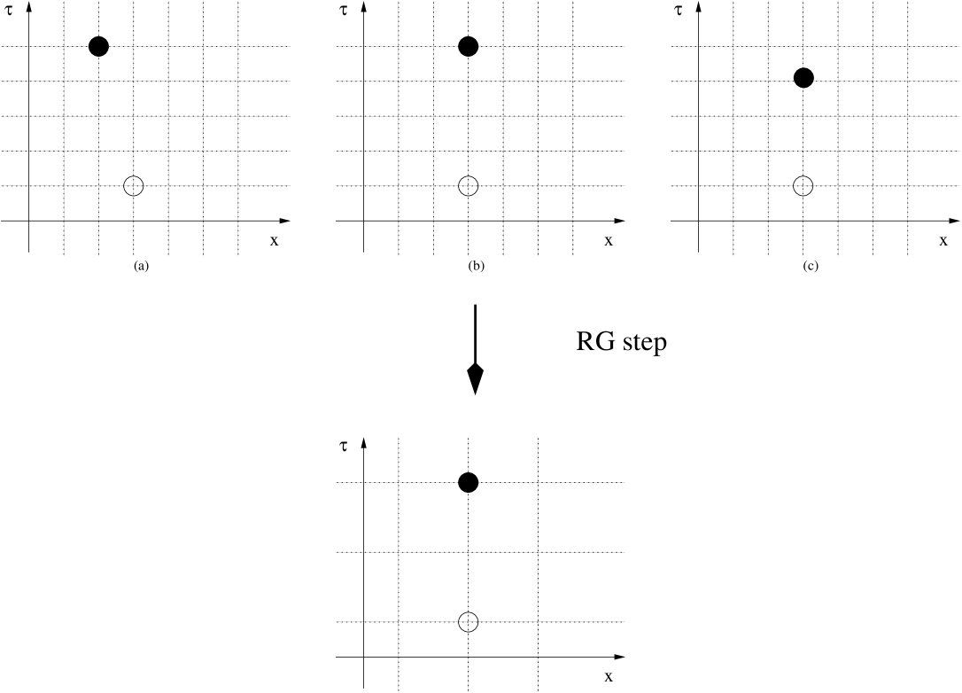
Figure 2: Length rescaling in the CG. Originally distinct charge configurations are identified at the new scale.

The first step consists of integrating large wavelength modes and then rescaling parameters so as to reconstruct the original action form.Shankar (1994) This corresponds to the overall length rescaling:

$$r_{ij}=\frac{\bar{r}_{ij}}{1-d\ell}$$ (14)

in the action and the partition function measure $D\eta$. Upon rescaling we lose the ability to distinguish certain previously distinct charge configurations as exemplified in Fig. 2. Applying Eq. (14) to the effective action Eq. (12) and expanding the logarithm for $d\ell\ll 1$, we obtain:

$$S_{eff} = \bar{S}_{eff}+\frac{1}{2}\sum_{i\neq j}\left[\frac{\kappa^{2}}{g_{\sigma}}m\left(\eta_{i}\right)m\left(\eta_{j}\right)\right.$$

$$+ \left.g_{\sigma}e\left(\eta_{i}\right)e\left(\eta_{j}\right)+g_{\rho}c\left(\eta_{i}\right)c\left(\eta_{j}\right)\right]d\ell.$$

The neutrality conditions can be used to rewrite the last term as a single sum over sites:

$$\bar{S}_{eff} = S_{eff}+\frac{1}{2}\sum_{i}\left[\frac{\kappa^{2}}{g_{\sigma}}m\left(\eta_{i}\right)^{2}\right.$$ (15)

$$+ \left.g_{\sigma}e\left(\eta_{i}\right)^{2}+g_{\rho}c\left(\eta_{i}\right)^{2}\right]d\ell.$$

The integral over $\eta$ is the sum over all possible particle positions, and its rescaling leads to:

$$d\eta_{i}=\frac{d\bar{\eta}_{i}}{\left(1-d\ell\right)^{d}}.$$ (16)

fugacity	$\left(m,e,c\right)$	Number of particles
$\tilde{G}=0$	$\left(\pm 2,0,0\right)$	$N_{4}$
$G=0$	$\left(0,\pm 2,0\right)$	$N_{5}$
$\Gamma=0$	$\left(0,0,\pm 2\right)$	$N_{6}$

Table 2: New particles created upon rescaling and their charges.

We have left the dimension $d$ unspecified for the following reason. Since a particle can only exist at the space coordinate where a spin exists, we can define two important limits in the KLM. If the Kondo spins are separated by a distance greater than $d\ell$, the sum over identical configurations is one dimensional $\left(d=1\right)$, as in the single impurity case (see $\left(b\right)$ and $\left(c\right)$ of figure 2). This is the dilute limit or “incoherent regime” of the Kondo lattice, where the scaling proceeds exactly as in the single impurity Kondo problem in a LL as found by Lee and Toner.Lee and Toner (1992) In contrast, when $d\ell$ is larger than the distance between Kondo spins we are in the dense limitZachar et al. (1996) or “coherent regime” of the Kondo lattice. In the latter case, the identification of initially distinct configurations can involve charges at different space coordinates, implying that $d=2$ (see $\left(a\right)$ in figure 2). We will focus on this coherent regime and set $d=2$ from now on.

Collecting Eqs. (15) and (16) we can express the partition function once again as a Coulomb gas by redefining the particle fugacities. A particle with charges $\left(m,e,c\right)$ has its fugacity $Y_{m,e,c}$ renormalized as

$$\frac{dY_{m,e,c}}{d\ell}=\left(2-\frac{1}{2}\left(\frac{\kappa^{2}}{g_{\sigma}}m^{2}+g_{\sigma}e^{2}+g_{\rho}c^{2}\right)\right)Y_{m,e,c}.$$ (17)

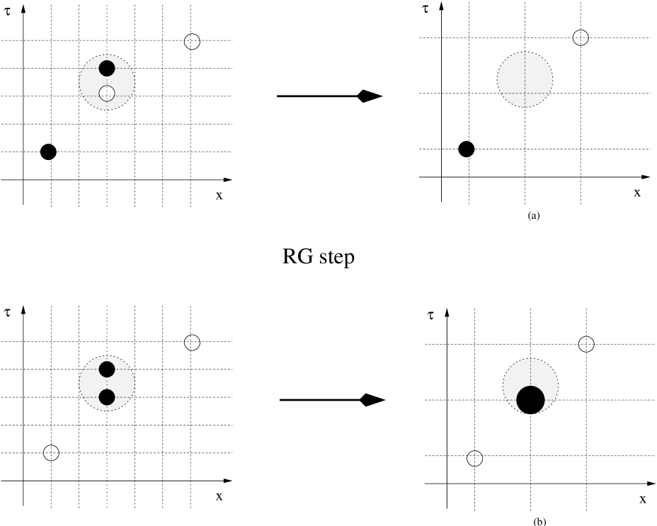
Figure 3: “Close pair” processes in the RG step: (a) particle annihilation and (b) particle fusion.

This equation gives the dimension of the corresponding operator and leads to the standard relevance criteria for bosonic operators. However, we have so far disregarded two possibilities. Suppose that a pair of initially distinct particles is within range of the new smallest scale. Following Anderson et al.Anderson et al. (1970) we call it a “close pair”. After the RG step we can no longer resolve these two particles as separate entities. On the one hand, if the particles have precisely opposite charges we have a “pair annihilation” (see (a) in Fig (3)). The residual dipole polarization of this pair renormalizes the interaction among the other particles, leading to the RG equations for $g_{\sigma}$ and $g_{\rho}$. Note that $\kappa$ is an RG invariant. On the other hand, if the pair is not neutral the particles are fused into a new particle carrying the net charge (see (b) in Fig (3)). This last process may actually create particles previously absent in the gas. There are three new kinds of particles created upon fusion in the dense limit with initial conditions $g_{\sigma}\sim g_{\rho}\sim 1$. Their charges and fugacities are listed in Tab. 2. These new entities correspond to originally marginal operators that are absent in the bare problem (their physical meaning will be discussed in the next section). Other particles with higher charges could also be considered, but from Eq. (17) it is clear that they are highly irrelevant and therefore can be neglected. Collecting the annihilation and fusion terms, derived in Appendix B, and adding the dimensionality equation (17), we complete the renormalization group equations. Away from half-filling, where the backward-scattering terms are irrelevant, particles with fugacities $y_{2,3}$ and $\Gamma$ can be disregarded. Thus, only configurations involving the fugacities $y_{1}$, $G$ and $\tilde{G}$ need to be considered. On the other hand, at half-filling all particles from Tabs. 1 and 2 should be included. This leads to the following renormalization group equations

• Away from half-filling

  $$\frac{dy_{1}}{dl} = \left(2-\frac{1}{2}\left(\frac{\kappa^{2}}{g_{\sigma}}+g_{\sigma}\right)\right)y_{1}+\frac{\sin\left(2\pi\kappa\right)}{2\kappa}y_{1}\left(G+\tilde{G}\right),$$

  $$\frac{dG}{dl} = 2\left(1-g_{\sigma}\right)G+\pi y_{1}^{2},$$

  $$\frac{d\tilde{G}}{dl} = 2\left(1-\frac{\kappa^{2}}{g_{\sigma}}\right)\tilde{G}+\pi y_{1}^{2},$$

  $$\frac{1}{2\pi^{2}}\frac{d\ln g_{\sigma}}{dl} = \frac{\sin\left(2\pi\kappa\right)}{4\pi\kappa}\left(\frac{\kappa^{2}}{g_{\sigma}}-g_{\sigma}\right)y_{1}^{2}+\frac{\kappa^{2}}{g_{\sigma}}\tilde{G}^{2}-g_{\sigma}G^{2},$$

  $$\frac{1}{2\pi^{2}}\frac{d\ln g_{\rho}}{dl} = 0.$$

• At half-filling

  $$\frac{dy_{1}}{dl} = \left(2-\frac{1}{2}\left(\frac{\kappa^{2}}{g_{\sigma}}+g_{\sigma}\right)\right)y_{1}+\frac{\sin\left(2\pi\kappa\right)}{2\kappa}y_{1}\left(G+\tilde{G}\right)+\pi y_{2}y_{3},$$

  $$\frac{dy_{2}}{dl} = \left(2-\frac{1}{2}\left(\frac{\kappa^{2}}{g_{\sigma}}+g_{\rho}\right)\right)y_{2}+\frac{\sin\left(\pi\kappa\right)}{\kappa}y_{1}y_{3}+\pi y_{2}\left(\tilde{G}+\Gamma\right),$$

  $$\frac{dy_{3}}{dl} = \left(2-\frac{1}{2}\left(g_{\sigma}+g_{\rho}\right)\right)y_{3}+\frac{\sin\left(\pi\kappa\right)}{\kappa}y_{1}y_{2}+\pi y_{3}\left(G+\Gamma\right),$$

  $$\frac{dG}{dl} = 2\left(1-g_{\sigma}\right)G+\pi\left(y_{1}^{2}+y^{2}_{3}\right),$$

  $$\frac{d\tilde{G}}{dl} = 2\left(1-\frac{\kappa^{2}}{g_{\sigma}}\right)\tilde{G}+\pi\left(y_{1}^{2}+y^{2}_{2}\right),$$

  $$\frac{d\Gamma}{dl} = 2\left(1-g_{\rho}\right)\Gamma+\pi\left(y^{2}_{2}+y^{2}_{3}\right),$$

  $$\frac{1}{2\pi^{2}}\frac{d\ln g_{\sigma}}{dl} = \frac{\sin\left(2\pi\kappa\right)}{4\pi\kappa}\left(\frac{\kappa^{2}}{g_{\sigma}}-g_{\sigma}\right)y_{1}^{2}+\frac{\kappa^{2}}{g_{\sigma}}\left(\tilde{G}^{2}+\frac{y^{2}_{2}}{2}\right)-g_{\sigma}\left(G^{2}+\frac{y^{2}_{3}}{2}\right),$$

  $$\frac{1}{2\pi^{2}}\frac{d\ln g_{\rho}}{dl} = -g_{\rho}\left(\frac{y^{2}_{2}}{2}+\frac{y_{3}^{2}}{2}+\Gamma^{2}\right);$$

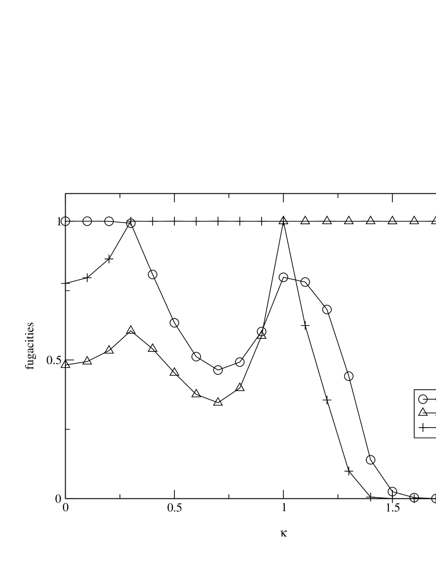
(a) Fugacities

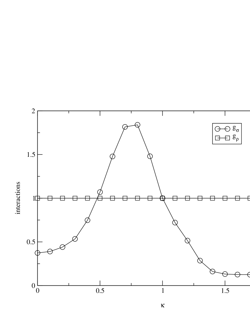
(b) Interaction constants

Figure 4: RG flow away from half-filling as a function of $\kappa$.

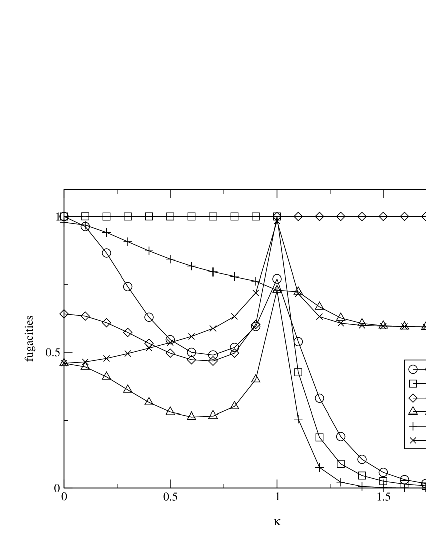
(a) Fugacities

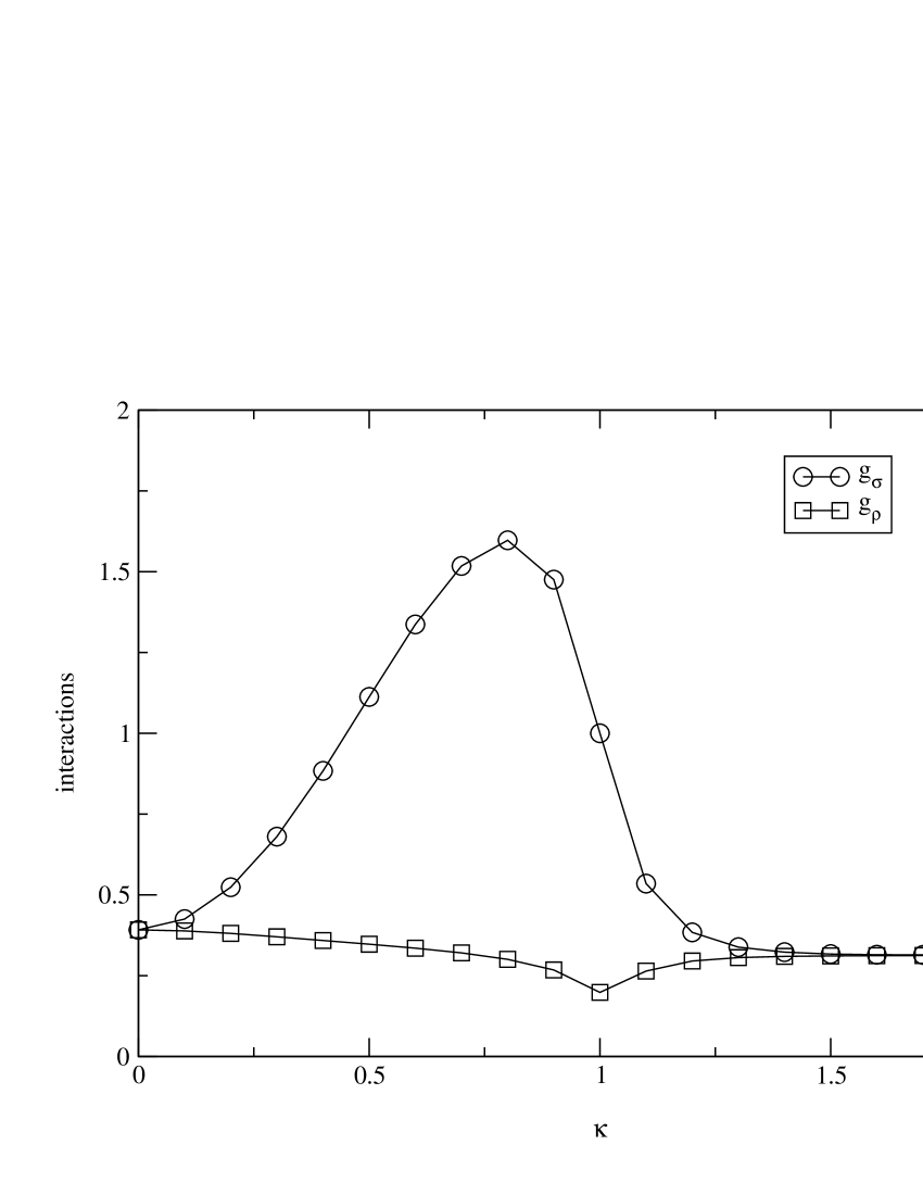
(b) Interaction constants

Figure 5: RG flow at half-filling as a function of $\kappa$.

A numerical solution of these sets of equations is shown in Fig. (4) and Fig. (5). For these particular plots we used $y_{1,2,3}\left(0\right)=0.01$, $g_{\sigma}\left(0\right)=g_{\rho}\left(0\right)=1$ and $\mathrm{G}\left(0\right)=\tilde{G}\left(0\right)=\Gamma\left(0\right)=0$. The RG flows were stopped when any of the fugacities reached the value of $1$ and the values of the other parameters were then plotted at this point. The flow equations depend only on the absolute value of $\kappa$.

As can be readily checked, the equations always flow to strong coupling. Nevertheless, special values of $\left|\kappa\right|$ allow us to trace regions with qualitatively different flows. Since the RG equations depend only on $\left|\kappa\right|$, those regions are mirror reflections on the $\kappa=0$ line, the “Toulouse line”.Zachar et al. (1996) For $\kappa^{2}>3$, single spin flip processes are irrelevant ($y_{1,2}\rightarrow 0$), just like in the FM single impurity Kondo problem.Anderson et al. (1970); Leggett et al. (1987) Moreover, the final flow is independent of the precise value of $\kappa$ , clearly indicating a distinct phase of the model. From now on, we will denote this phase as region $1$. In contrast, spin flips are always relevant for $\left|\kappa\right|<3$, but we also encounter a second special flow. For $\left|\kappa\right|=1$, the particle fugacities $G$ and $\tilde{G}$ are always the same. There is also a precise balance between the “magnetic” ($\kappa^{2}/g_{\sigma}$) and “electric” ($g_{\sigma}$) interactions. Consequently, the ground state is a plasma for particles of type $\left(m,e,0\right)$, implying that $\phi_{s}$ and $\theta_{s}$ are completely disordered. In fact, $\kappa=1$ corresponds to the critical point of the problem of two weakly coupled LL’s. Therefore, we can safely identify $\left|\kappa\right|=1$ as a boundary between different phases. For other values of $\left|\kappa\right|$ the interactions are screened ($g\rightarrow 0\,\textrm{or}\,\infty$) and/or the fugacities have different flows. It is clear that for $1<\kappa^{2}<3$ (denoted as region $2$) single-spin-flip fugacities become less and less relevant as $\kappa^{2}\to 3$. This suggests a transition region from the disordered state at $\left|\kappa\right|=1$ to the flow of region $1$. We shall call $\left|\kappa\right|<1$ region $3$. In contrast to the previous cases, single flips are always strongly relevant in this region. The order of relevance of the fugacities changes a few times as $\kappa$ is varied in this region. However, a particularly simple case occurs in the “Toulouse line” ($\kappa=0$).

Even though the renormalization flows are clear and the special flows were identified, their physical interpretation is less straightforward. In order to proceed we must assign a physical meaning to each particle in the gas, from which we can then attempt to determine the phase diagram.

V Effective Hamiltonians

At each RG step we rewrote the problem as a CG. Moreover, all the neutrality conditions were preserved by the RG step. We therefore can define a quantum Hamiltonian that reproduces the CG at each step. This effective Hamiltonian allows us to understand the behavior of the system and, in certain special cases, to infer its phase.

In the dense limit of the KLM, the distance between localized spins is of the order of the smallest bosonic wavelength available. Therefore, after the first RG step we were forced to introduce new entities in the problem. Their Hamiltonian form is trivially guessed from their definitions,

$$O_{1} \sim \tilde{G}\left[F^{\dagger}_{R\uparrow}F^{\phantom{\dagger}}_{R\downarrow}F^{\dagger}_{L\uparrow}F^{\phantom{\dagger}}_{L\downarrow}\right.$$ (18a)

$$\left.e^{i\left|\kappa\right|\sqrt{\frac{8\pi}{g_{\sigma}}}\theta_{s}\left(x\right)}S^{-}\left(x+\delta\right)S^{-}\left(x\right)+h.c.\right],$$

$$O_{2} \sim G\left[F^{\dagger}_{R\uparrow}F^{\phantom{\dagger}}_{R\downarrow}F^{\dagger}_{L\downarrow}F^{\phantom{\dagger}}_{L\uparrow}\right.$$ (18b)

$$\left.e^{i\sqrt{8\pi g_{\sigma}}\phi_{s}\left(x\right)}S^{+}\left(x+\delta\right)S^{-}\left(x\right)+h.c.\right],$$

$$O_{3} \sim 4\Gamma\sum_{\left\{\eta\neq\nu\right\}=R,L}\sum_{\left\{\sigma_{1},\sigma_{2}\right\}=\uparrow,\downarrow}\left[F^{\dagger}_{\eta\sigma_{1}}F^{\phantom{\dagger}}_{\nu\sigma_{1}}F^{\dagger}_{\nu\sigma_{2}}F^{\phantom{\dagger}}_{\eta\sigma_{2}}\right.$$ (18c)

$$\left.e^{i\sqrt{8\pi g_{\rho}}\phi_{c}\left(x\right)+4ik_{F}x}S^{z}\left(x+\delta\right)S^{z}\left(x\right)+h.c.\right],$$

where $\delta$ is a distance of the order of the inverse of the bosonic cut-off $\left(\sim\alpha\right)$. Both the $O_{1}$ and the $O_{2}$ terms involve simultaneous flips of two nearby spins and the creation of particles with charges $(m,e,c)=(\pm 2,0,0)$ and $(0,\pm 2,0)$, respectively. In contrast, $O_{3}$ is not related to spin flips and generates particles with charges $\left(0,0,\pm 2\right)$. It is simple to understand their origin. In the original Hamiltonian of Eq. (2), it is possible to spatially resolve the fermion-spin scattering events . As we reduce the bosonic cut-off this is no longer true, and we must consider multiple scattering events within the new smallest scale, $\alpha$. There are clear similarities between the conduction electron operators in Eqs. (18) and the usual backscattering and Umklapp operators. The standard picture of the RKKY interaction is that of an effective spin-spin interaction mediated by the conduction electrons. In light of Eqs. (18), it seems natural to consider also the opposite point of view: an indirect electron-electron interaction mediated by the local spins. The RG procedure introduces these composite events in a natural fashion.

The final operator that must be introduced in the effective Hamiltonian is a result of the annihilation process. Unlike fusion, when a pair is annihilated the zeroth order term in an Operator Product Expansion of the bosonic fields is a constant. Nevertheless, it is still a function of the local spins and must be considered at the last RG step in order to establish an effective Hamiltonian. Collecting all possible pair annihilation terms and expanding point-split bosonic operators we get

$$O_{z} \sim 4\left(\tilde{G}^{2}-G^{2}\right)S^{z}\left(x+\delta\right)S^{z}\left(x\right)$$ (19)

$$+ \left(y_{1}^{2}+y_{2}^{2}\right)S^{-}\left(x+\delta\right)S^{+}\left(x\right)+\mathrm{h}.\,\mathrm{c}.$$

It must be stressed that the spin operators in Eqs. (18) and (19) should not be understood as the original local spins. Consider the spin history of Fig 6 as an example. Suppose that the pair flip-antiflip is produced by a forward $J_{\perp}^{f}$ term and a backward $J_{\perp}^{b}$ term at times $\tau$ and $\tau+\delta$ within the new renormalization scale. This is equivalent to having no flip at all and cannot be distinguished from a particle with fugacity $J_{z}^{b}$. At the operator level, this is formally accomplished by summing over all possible products of flip operators, expanding the result in $\delta\sim\alpha$ and reordering the Klein factors. The latter are actually crucial for the correct final sign (see Appendix C for details). Thus, we exactly reproduce the $z$-backscattering particle by defining the $S^{z}$ spin at the new scale as

$$2S^{z}\left(\bar{x},\bar{\tau}\right)\equiv S^{+}\left(x,\tau+\delta\right)S^{-}\left(x,\tau\right)-S^{-}\left(x,\tau+\delta\right)S^{+}\left(x,\tau\right).$$

A similar calculation can be done for any other possible spin history and bosonic operator within a disk of radius $\delta\sim\alpha$. Therefore, the local spins in the effective Hamiltonian represent block spins (as in the example above) and not the original ones.

Figure 6: Two different spin histories at the older RG scale that cannot be distinguished at the new one.

Taking $\delta$ as the lattice spacing at the last RG step and collecting all these operators, we find the effective Hamiltonian

$$H_{eff} = H_{0}+\sum_{j}\left\{4\left[\tilde{G}^{2}-G^{2}\right]+8\Gamma\cos\left(\sqrt{8\pi g_{\rho}}\phi_{c}\left(x_{j}\right)+4k_{F}x_{j}\right)\right\}S^{z}\left(x_{j+1}\right)S^{z}\left(x_{j}\right)$$ (20)

$$+ 8y_{3}\sin\left(\sqrt{2\pi g_{\rho}}\phi_{c}\left(x_{j}\right)+2k_{F}x_{j}\right)\sin\left(\sqrt{2\pi g_{\sigma}}\phi_{s}\left(x_{j}\right)\right)S^{z}\left(x_{j}\right)$$

$$+ 2\left[y_{1}\cos\left(\sqrt{2\pi g_{\sigma}}\phi_{s}\left(x_{j}\right)\right)+y_{2}\cos\left(\sqrt{2\pi g_{\rho}}\phi_{c}\left(x_{j}\right)+2k_{F}x_{j}\right)\right]e^{i\sqrt{\frac{2\pi}{g_{\sigma}}}\kappa\theta_{s}\left(x_{j}\right)}S^{+}\left(x_{j}\right)$$

$$+ \left[Ge^{i\sqrt{8\pi g_{\sigma}}\phi_{s}\left(x_{j}\right)}+y_{1}^{2}+y_{2}^{2}\right]S^{+}\left(x_{j+1}\right)S^{-}\left(x_{j}\right)$$

$$+ \tilde{G}e^{i\sqrt{\frac{8\pi}{g_{\sigma}}}\kappa\theta_{s}\left(x_{j}\right)}S^{+}\left(x_{j+1}\right)S^{+}\left(x_{j}\right)+\mathrm{h}.\,\mathrm{c}.$$

VI 1D anisotropic KLM phase diagram

For certain values of $\kappa$ the effective Hamiltonian in Eq. (20) is independent of the bosonic fields at the end of the RG flow. We will exploit these cases to intuit the various phases of the model.

We start by considering the system away from half-filling, where $y_{2,3}$ are irrelevant and $\Gamma\equiv 0$. The RG flows are summarized in Table 3.

Region	$y_{1}$	$G$	$\tilde{G}$	$\tilde{G}-G$
1	$\rightarrow 0$	$\rightarrow\infty$	$0$	$<0$
2	$\rightarrow\infty$	$\rightarrow\infty$	$\rightarrow\infty$	$<0$
3	$\rightarrow\infty$	$\rightarrow\infty$	$\rightarrow\infty$	$>0$

Table 3: RG flows for the fugacities away from half-filling.

In region 1, the only relevant fugacity is $G$. Therefore, $\sqrt{8\pi g_{\sigma}}\phi_{s}$ freezes at $\pi$. This reduces Eq. (20) to the anisotropic ferromagnetic Heisenberg model

$$H_{eff} \sim \sum_{j}\left(-4G^{2}\right)S^{z}\left(x_{j+1}\right)S^{z}\left(x_{j}\right)$$

$$- G\left[S^{+}\left(x_{j+1}\right)S^{-}\left(x_{j}\right)+S^{+}\left(x_{j}\right)S^{-}\left(x_{j+1}\right)\right]$$

in its ordered phase ($G\sim 1,\left\langle S^{z}\right\rangle=1/2$).

The effective Hamiltonian for the $\kappa=0$ line, the “Toulouse” line, is also independent of the bosonic field. Since the most relevant fugacity is $y_{1}$, $\sqrt{2\pi g_{\sigma}}\phi_{s}$ freezes at $\pi$. This leads to an antiferromagnetic XYZ model in an external field

$$H_{eff} \sim \sum_{j}2\left[\tilde{G}^{2}-G^{2}\right]S^{z}\left(x_{j+1}\right)S^{z}\left(x_{j}\right)-4y_{1}S^{x}\left(x_{j}\right)$$ (22)

$$+ \left(\frac{y_{1}^{2}+G+\tilde{G}}{2}\right)S^{x}\left(x_{j+1}\right)S^{x}\left(x_{j}\right)$$

$$+ \left(\frac{y_{1}^{2}+G-\tilde{G}}{2}\right)S^{y}\left(x_{j+1}\right)S^{y}\left(x_{j}\right).$$

In this case, the effective spin Hamiltonian exhibits order in the XY plane, $G\sim\widetilde{G}\sim y\sim 1$. Nevertheless, this does not imply any order of the original spins. As we stated before, all our results must be understood in the rotated basis of Eq. (13). This ensures that the original model, Eq. (2), is still disordered, as emphasized in Ref. Zachar et al., 1996. Therefore, the system is paramagnetic with short range antiferromagnetic correlations. Although the “Toulouse line” corresponds to a particular case, it seems reasonable to extend this assignment to the entire region $3$. For one thing, because the first term in Eq. (22), which drives the antiferromagnetic tendency, remains positive throughout this region. Besides, the XY disordering terms are the dominant interaction in the region. In particular, in the $\left|\kappa\right|=1$ line, the symmetric flow of $G$ and $\tilde{G}$ ensures that the $z$-term vanishes and therefore the order parameter $\left\langle S^{x,y,z}\right\rangle$ is still zero. Hence, we propose that the entire region 3 is a paramagnetic phase with short range antiferromagnetic correlations. Note that this is not necessarily true for other observables, since the flows near $\left|\kappa\right|=0$ and $\left|\kappa\right|=1$ are qualitatively different.

There is no simple effective Hamiltonian within region 2, but the disordering term, proportional to $y_{1}$, becomes progressively less relevant as $\kappa^{2}\to 3$. More importantly, the short range $z$ correlations turn from antiferro- to ferromagnetic. Consistent with the identification of region $1$ as a ferromagnetic phase, these two features lead us to tentatively identify region 2 as a ferromagnetically ordered phase with unsaturated magnetization of the spins.

Collecting these results, we conclude that there are at least two continuous phase transitions in the anisotropic KLM far from half-filling. The first transition, from region 1 to region 2 in Fig. 7, reminiscent of the Berezinskii-Kosterlitz-Thouless transition of the single impurity Kondo model,Anderson et al. (1970) separates regions of relevance and irrelevance of the single flip process. The effective model for region 1, Eq. (VI), has ferromagnetic order with full saturation of the localized spins. A regime with ferromagnetic order, however, is beyond the present bosonization treatment, since the spin polarization of the conduction electrons leads to different Fermi velocities for up and down spin electrons. However, the RG flow is still able to indicate its existence through the irrelevance of single spin flips and the nature of the effective Hamiltonian (VI). Ferromagnetism is simple to understand in the strong coupling limit ($\left|J_{z}\right|\gg J_{\perp}$). In this case, ferromagnetic ordering allows the electrons to lower their kinetic energy. In fact, this picture seems to survive down to the isotropic case both for $J_{z}>0$Sigrist et al. (1991); Tsunetsugu et al. (1997) and $J_{z}<0$.Dagotto et al. (1998) In the FM case, this mechanism is well established and is usually called double exchange. However, in the AFM chain this simple image of an up-spin electron moving in a background of localized down-spins is no longer valid (as can be analytically checked in the Kondo lattice with one electronSigrist et al. (1991); Tsunetsugu et al. (1997)). In the latter, the objects that lower the kinetic energy are actually the Kondo singlets. Following this argument, the total spin per site (electrons+spins) would be $S_{tot}^{z}=\left\langle S^{z}\right\rangle-n_{c}/2=(1-n_{c})/2$ in the antiferromagnetic case and $S_{tot}^{z}=(1+n_{c})/2$ in the ferromagnetic one, as observed numerically.Tsunetsugu et al. (1997); Dagotto et al. (1998)

There is another continuous phase transition line from region 2 to region 3 in Fig. 7, similar to the transition of the Ising model in a transverse field,Kogut (1979) that separates a paramagnetic phase (region 3 of Fig. 7) from a region with unsaturated magnetization of the localized spins. The magnetization grows continuously up to the border of region 1. It is tempting to identify region 2 with similar phases with unsaturated moments found in numerical studies of both the isotropic FM KLM of Dagotto et al.Dagotto et al. (1998) and the isotropic AFM KLM of Tsunetsugu et al.Tsunetsugu et al. (1997)

The numerical studies of the FM KLM also identified a region of phase separation.Dagotto et al. (1998) We did not find any indication of phase separation. We can think of two reasons why. First, the coupling constant in that region is of the order of the electron bandwidth and therefore bosonization is no longer valid. Moreover, this phase is a competition between the ferromagnetic tendencies of lower band fillings and the antiferromagnetic counterpart at half-filling. Since we completely neglect backscattering (ultimately responsible for the antiferromagnetism) this phase was lost even before we began.

Figure 7: Phase diagram of the 1D anisotropic KLM away from half-filling. Regions 1 are fully polarized ferromagnets, regions 2 are partially polarized ferromagnets and regions 3 are paramagnetic. See text for details.

As we pointed out before, at half-filling we are able to include the backscattering terms in the RG scheme. We will now consider this case. The first result from the RG flow is that $O_{3}$, whose bosonic part is identical to an Umklapp term, is always relevant, pointing to the presence of a charge gap. The spin sector is more subtle and we must consider some special cases.

Region 1 can be simply analyzed. The interaction parameters $g_{\sigma}$ and $g_{\rho}$ go to zero and the most relevant fugacity is $y_{3}$. Therefore, $\sqrt{2\pi g_{\rho}}\phi_{c}$ freezes at $\frac{\pi}{2}$. The other relevant flows are $\Gamma$ and $G$. The effective Hamiltonian reduces to an anisotropic ferromagnetic Heisenberg model in a staggered field,

$$H_{eff} \sim \sum_{j}\left(-4G^{2}-8\Gamma\right)S^{z}\left(x_{j+1}\right)S^{z}\left(x_{j}\right)$$

$$- GS^{+}\left(x_{j+1}\right)S^{-}\left(x_{j}\right)+\mathrm{h}.\,\mathrm{c}.$$

$$+ \left(-1\right)^{x_{j}}8y_{3}S^{z}\left(x_{j}\right).$$

The staggered field induces Néel order, but the system has strong ferromagnetic tendencies. As we move away from half-filling, the staggered field becomes progressively irrelevant and the ferromagnetic effective model is reobtained.

The $\kappa=0$ point is once again very special. At the end of the RG flow, the effective Hamiltonian is also free of the bosonic fields and the most relevant fugacities are $y_{2}$ and $y_{1}$. They force $\sqrt{2\pi g_{\rho}}\phi_{c}$ and $\sqrt{2\pi g_{\sigma}}\phi_{s}$ to freeze at $\pi$, suppressing the staggered field in the $z$ direction. Thus, the “Toulouse point” effective Hamiltonian is

$$H_{eff} \sim \sum_{j}\left[2\left(\tilde{G}^{2}-G^{2}\right)+4\Gamma\right]S^{z}\left(x_{j+1}\right)S^{z}\left(x_{j}\right)$$

$$- \left(\frac{G+y_{1}^{2}+y_{2}^{2}+\tilde{G}}{2}\right)S^{x}\left(x_{j+1}\right)S^{x}\left(x_{j}\right)$$

$$- \left(\frac{G+y_{1}^{2}+y_{2}^{2}-\tilde{G}}{2}\right)S^{y}\left(x_{j+1}\right)S^{y}\left(x_{j}\right)$$

$$- 4\left(y_{1}+\left(-1\right)^{x_{j}}y_{2}\right)S^{x}\left(x_{j}\right).$$

As before this does not imply any order of the original spins in the XY plane. From this effective model we can see that the $\left|\kappa\right|=0$ point is characterized by spin and charge gaps and no ordering.

In summary, at half filling we assign two distinct magnetic phases. Regions $1$ and $2$ have Néel order in the $z$ direction. On the other hand, if we assume that the “Toulouse line” features can be extended to the entire region $3$, we can identify this region with a paramagnetic phase. The several changes in the relative flows maybe a sign of additional phases as a function of $\kappa$. However, the effective Hamiltonian cannot be so easily solved and we are unable to make further progress.

The KLM at half-filling was studied by Shibata et al.Shibata et al. (1995) By looking at the strong coupling limit, they were able to find five distinct magnetic phases, which they argue survive down to weak coupling: two Néel phases (FM and AFM), a planar phase (the triplet state with $S^{z}=0$), a Haldane phase and a Kondo singlet (paramagnetic) phase. Because of the relevance of backscattering and the condition $\tilde{J}_{z}^{b}\ll 1$, a direct comparison between the RG flows and the available numerical results is restricted to $\kappa\sim 1$. This neighborhood has no simple effective Hamiltonian and we are unable to make direct contact with the numerical results. We can point out, however, that the strong coupling flow of $g_{\sigma}$ is an indication of the opening of a spin gap, though this is less certain because of the difficulty of analyzing the effective Hamiltonian. This possible spin gap is compatible with the Haldane type phase at $J_{z}<0$ and the Kondo singlet phase at $J_{z}>0$ obtained in Ref. Shibata et al., 1995. As we dope the system away from half-filling the backward-scattering terms become irrelevant, and a direct comparison with the numerical data becomes more feasible.

As a final illustration of the usefulness of the Coulomb gas mapping, we develop in Section VII its application to a related yet simplified model of spins and fermions: the Ising-Kondo chain. Its simplicity makes it a more pedagogical example of the formalism.

VII The Ising-Kondo chain

The Ising-Kondo model,

$$H=\sum_{\vec{k},\sigma}\varepsilon_{\vec{k}}\psi^{\dagger}_{\vec{k},\sigma}\psi_{\vec{k},\sigma}+J\sum_{i,s,\acute{s}}S_{i}^{z}\psi^{\dagger}_{i,s}\frac{\sigma_{s,\acute{s}}^{z}}{2}\psi_{i,\bar{\sigma}}+y\sum_{i}S_{i}^{x},$$

was proposed by Sikkema et al.Sikkema et al. (1996) as a model for the weak antiferromagnetism of $\mathrm{URu}_{2}\mathrm{Si}_{2}$. Here, we will consider the one dimensional version of this model and apply the same methods that we used in the Kondo chain. Using bosonization and disregarding the backscattering terms, the Hamiltonian simplifies to

$$H=H_{0}+\sum_{i}\sqrt{\frac{2}{\pi}}\tilde{J}\partial_{x}\phi\left(i\right)S^{z}\left(i\right)-\tilde{y}S^{x}\left(i\right),$$ (23)

where the coupling constants were rescaled by the Fermi velocity as before. Eq. (23) is identical to the co-operative Jahn-Teller Hamiltonian.Gehring and Gehring (1975) The lower symmetry of the model allows us to foresee that the sign of $J$ is irrelevant to the physics. It is also a well known result from the co-operative Jahn-Teller problem that the strong coupling limits $\tilde{J}\gg 1$ and $\tilde{y}\gg 1$ show easy axis order in the $z$ and $x$ directions, respectively.

Exactly as in the KLM, we can proceed by going to a path integral formulation with bosonic coherent states and the local spin $S_{z}$ basis. After tracing the bosonic fields and integrating by parts the spin variables, the Coulomb gas that follows has only one breed of particles $\left(m,0,0\right)$, subjected to the neutrality condition 1 of Section II. To mimic our previous notation we define $g=\sqrt{\frac{2\pi}{J}}$. Assuming $\tilde{y}\ll 1$, the RG equation can be derived in a similar fashion. They correspond to the standard Kosterlitz-Thouless equations,

$$\frac{dy}{dl} = 2\left(1-g\right)y,$$

$$\frac{d\ln g}{dl} = -gy^{2}.$$

For $g>1$, spin flip processes are irrelevant (see Fig. 8, region 1). In the Jahn-Teller language this corresponds to a ferrodistortion of the $y\ll J$ fixed point. On the other hand, for $g<1$ spin flips are relevant, $y\rightarrow\infty$ and $g\rightarrow 0$ (see Fig. 8, region 2). We can find an effective Hamiltonian to shed light on the physics in this regime. Indeed, we could have applied the rotation in Eq. (13) to the original Hamiltonian to get

$$H=H_{0}-\frac{y}{2}e^{-i\sqrt{8\pi g}\theta\left(x_{i}\right)}S^{+}\left(x_{i}\right)+\mathrm{h}.\,\mathrm{c}.+\mathrm{s}.\,\mathrm{r}.\,\mathrm{t}.,$$

where “s. r. t.” stands for “short range terms”. The operators in this rotated basis are called “displaced” in the co-operative Jahn-Teller literature.Gehring and Gehring (1975) This rotation is equivalent to the integration by parts of the $S_{z}$ variables in the time direction, as we saw. By taking now $y\rightarrow\infty$ and $g\rightarrow 0$, the effective Hamiltonian is simply a magnetic field in the $x$ direction acting to order the local spins. Unlike in the KLM, the original spins are also ordered in the $x$ direction since $\theta$ freezes at the value of zero. The transition is continuous and of the Kosterlitz-Thouless type.

Figure 8: Phase diagram of the Ising-Kondo chain. In Region 1 the transverse field is irrelevant, while in Region 2 it is relevant. See text for details.

VIII Discussion and Conclusions

We have proposed in this article what is the natural extension to the one-dimensional lattice of the highly successful approach of Anderson, Yuval and HammanAnderson and Yuval (1969); Yuval and Anderson (1970); Anderson et al. (1970) to the single impurity Kondo problem. The mapping to a Coulomb gas is made specially easy by using bosonization methods and particularly subtle developments demonstrate the importance of a careful consideration of Klein factors, so often neglected in most treatments.von Delft and Schoeller (1998) Since bosonization relies on the linearization of the conduction electron dispersion and is appropriate for the analysis of the long-wavelength physics it is never quite obvious how far it can be taken in its application to lattice systems. However, motivated by its success in the Hubbard, Heisenberg and other models, it is reasonable to attempt a direct comparison of our treatment to the phases of the anisotropic Kondo lattice model.

One of the hardest tasks in our treatment is the extraction of physical information from the effective models we obtain after several rescaling steps. Some special lines in the phase diagram can be more confidently analyzed, but as is common in RG treatments, we are then forced to attempt an extrapolation to other regions based on continuity arguments. This is specially true in our case, where most of the flows are towards strong coupling. Given these caveats, however, the overall topology of the phase diagram away from half-filling is compatible with the known phases of the isotropic model.Tsunetsugu et al. (1997); Dagotto et al. (1998) The extension of these studies to the anisotropic case would be highly desirable. At half-filling, the method itself limits its application to the $J_{z}\ll t$ region. Unfortunately, this is one of the regions where the effective Hamiltonian is hard to solve and we are not able to explore the rich phase diagram obtained in Ref. Shibata et al., 1995. Nevertheless, we do find a charge gap at half-filling throughout the phase diagram, which seems compatible with the numerical results. The question of the spin gap is less clear but our results are also compatible with what is known numerically.

We would also like to try to make contact with previous studies of the Kondo lattice model in one dimension based on the use of Abelian bosonization. In the important work of Zachar, Kivelson and Emery,Zachar et al. (1996) where the rotation of Eq. (13) is first used, the highly anisotropic “Toulouse line” ($\kappa=0$) is analyzed in detail. One of their findings is the presence of a spin gap in the spectrum away from half-filling, which also appears in our effective Hamiltonian. At half-filling, they also find spin and charge gaps, which seem compatible with our results. They also point out that the metal-insulator transition as $n\to 1$ is of the commensurate-incommensurate type.H. J. Schulz (1980) In our treatment, the commensurability condition $4k_{F}a=2\pi n=1$ for the relevance of the backward scattering terms, the same as in the Hubbard model, is a strong indication that the transition is indeed of this type.

Honner and Gulácsi have also investigated the spin dynamics of the isotropic Kondo chain.Honner and Gulácsi (1997, 1998) After smearing out the discontinuity in the commutation relations of the bosonic fields, they replace the latter by their expectation value in the non-interacting ground state and write an effective Hamiltonian for the localized spins. This Hamiltonian can then be treated numerically and the phase diagram determined. This procedure requires the fitting of the smearing length scale to numerical results. One of the advantages our treatment brings to the problem is the ability to do the full analysis analytically and without any a priori assumption about the boson dynamics. In fact, the Coulomb gas mapping treats spins and bosons on the same footing. Besides, no fitting to numerical results is necessary. A discrepancy between our results and those of Honner and Gulácsi is the partially polarized FM phase we find at $J_{z}<0$. In their treatment, a PM phase is found instead. It would be interesting to extend their treatment to the anisotropic case for a fuller comparison.

Recently, ZacharZachar (2001) conceived an alternative approach to the KLM in the rotated basis. He used a particular example of the rotation in Eq. (13)

$$\bar{U}=e^{i\sqrt{2\pi}\sum_{x}\theta_{s}\left(x\right)S^{z}\left(x\right)},$$

and treated the KLM in a self-consistent mean-field approximation. This approach led him to predict three different phases in the AFM KLM as well. The first region is controlled by the paramagnetic “Toulouse line” fixed point. In the rotated basis, this phase is characterized by $\left\langle S^{z}\left(x\right)\right\rangle=0$ and $\left\langle S^{x}\neq 0\right\rangle$, precisely as we find in region $3$ of Fig. 7. Another phase has $\left\langle S^{z}\right\rangle\neq 0$ and $\left\langle S^{x}\right\rangle=0$. In this case, the system exhibits ferromagnetic order in the original basis, and therefore could be identified with region $1$ of Fig. 7. Finally, embedded between these two phases, he also finds a third intermediate region, which he identifies as a “soliton lattice”, with $\left\langle S^{z}\right\rangle\neq 0$ and $\left\langle S^{x}\right\rangle\neq 0$. It is tempting to associate this intermediate phase with region 2 of Fig. 7. However, Zachar proposes a different description calling region 1 a “staggered liquid Luttinger liquid”, whereas we find it much more natural to associate $\left\langle S^{z}\right\rangle\neq 0$ with ferromagnetic order. He also conjectures that region $2$ does not exist. Finally, he argued that all transitions are first order and of the commensurate-incommensurate type, while we find them to be continuous.

In conclusion, we have presented a flexible treatment of a one-dimensional system of spins and fermions based on a mapping to a Coulomb gas, which we treat within a renormalization group approach. When applied to the Kondo lattice model, the method enables us to identify its various phases both at and away from half-filling.

Appendix A Neutrality Conditions for the KLM

Neutrality conditions are common in Coulomb gas formulations of quantum problems. In the simplest applications, these conditions impose that the overall charge is zero as, for instance, in the sine-Gordon model.Gogolin et al. (1998); Nienhuis (1987) As applied to our case this condition reads

$$\sum_{i}m\left(x_{i},\tau_{i}\right)=\sum_{i}e\left(x_{i},\tau_{i}\right)=\sum_{i}c\left(x_{i},\tau_{i}\right)=0.$$ (24)

They are the mathematical expression of the condition for the bosonic correlation functions not to vanish in the thermodynamic limit and they also ensure the overall cancellation of the Klein factors. However, in the KLM the presence of both spins and bosons leads to more stringent neutrality conditions than in other problems. Therefore, besides Eq. (24), there are two additional restrictions.

The first one comes from the impossibility of performing two consecutive upward spin flips on a given localized spin-$\frac{1}{2}$ site. Since, from Eq. (6) the $m=\pm 1$ variable gives the direction of a spin flip, it follows that $m$ must alternate in time. This condition is also present in the Coulomb gas formulation of the single impurity Kondo problem.Anderson and Yuval (1969) As a direct consequence of the alternation of the charge $m$ and the periodic boundary conditions in imaginary time, we obtain the first “strong” neutrality condition: the total charge $m$ at a given spatial position is zero $\sum_{i}m\left(x_{fixed},\tau_{i}\right)=0$. This gives condition 1 of Section II, whereas condition 2 is already contained in Eq. (24).

The second additional restriction is slightly less obvious. From Eq. (7), we see that each contribution to the partition function has a prefactor sign that depends on a string of Klein factors and $S^{z}$ operators, the latter coming from $z$ backward-scattering events generated by $H^{b}_{z}$ of Eq. (3d). The neutrality condition we will derive comes from the cancellation of terms with identical absolute values but with opposite prefactor signs. This will finally lead to condition 3 of Section II. We will now consider different cases separately.

Let us first focus on the contributions to the partition function coming from terms with forward scattering only (Eqs. (3b) and (3c)). If there are no spin flips, then the prefactor is obviously positive. When there is a pair of opposite flips (the only possibility allowed by the neutrality condition 1), then, because of the overall neutrality condition 2, the Klein factors cancel

$$F_{\eta\sigma_{1}}^{\dagger}F_{\eta\sigma_{2}}F_{\eta\sigma_{2}}^{\dagger}F_{\eta\sigma_{1}}=1,$$

preserving the positive sign. Consideration of configurations with additional pairs of flips leads to the same cancellation of Klein factors.

Next, we look at contributions generated by $H^{b}_{\perp}$(Eq. (3e)) only. By considering again increasing numbers of pairs of opposite flips as in the previous paragraph we arrive at an analogous cancellation of Klein factors.

Moving on now to contributions coming from $H_{z}^{b}$ (Eq. (3d)), we first consider the possibility of no spin flips. In this case, integrating out the bosonic modes, the contribution to the partition function is

$$z\sim\frac{e^{\pm 2ik_{F}\Delta x_{ij}}}{r^{g_{\rho}+g_{\sigma}}_{ij}}S^{z}\left(i\right)S^{z}\left(j\right),$$ (25)

where the Klein factors also cancel nicely. Tracing over the spin variables leads to no contribution to the partition function sum, unless $i$ and $j$ have the same space coordinate. What happens for a higher number of insertions of $H_{z}^{b}$ ? For the general case of $N$ particles coming from $H_{z}^{b}$, the contribution to the partition function will be

$$z\sim e^{\sum_{ij}\ln\left|r_{ij}\right|\left(g_{\rho}c_{i}c_{j}+g_{\sigma}e_{i}e_{j}\right)}\prod_{i}e^{2ik_{F}c_{i}x_{i}}S^{z}\left(i\right).$$

Note how each $S_{z}$ insertion comes with a corresponding $c$ charge. Thus, it is simple to show that tracing over $S_{z}\left(i\right)$ leads to the condition of having an even number of particles of charge $c$ at each spatial coordinate. Moreover, the reordering of Klein factors leads to their complete cancellation.

In order to generalize this result to a configuration with an arbitrary number of spin flips let us assume initially that there are only flips of one kind: either $H^{f}_{\perp}$ or $H^{b}_{\perp}$. By using the identity (using Pauli matrices instead of spin operators)

$$\sigma_{1}F_{\eta\sigma}^{\dagger}F_{\nu\sigma}F_{\xi\sigma_{1}}^{\dagger}F_{\psi\sigma_{2}}=\sigma_{2}F_{\xi\sigma_{1}}^{\dagger}F_{\psi\sigma_{2}}F_{\eta\sigma}^{\dagger}F_{\nu\sigma},$$ (26)

with $\nu\neq\eta$ and $\sigma_{1}\neq\sigma_{2}$, it is easy show that an $H_{z}^{b}$ insertion on one side of a domain wall can be moved to the other side with a sign change (see Fig. 9). Now consider, for example, a pair of particles generated by $H_{z}^{b}$ as before. When there is a pair of flips lying along the time line, we can move the Klein factors and $S^{z}$ through the domain walls with the identity above and cancel them out. Therefore, our previous result, obtained without the flips, remains valid. This can be generalized for any number of flips. Finally, we must consider the possibility of having flips coming both from $H_{\perp}^{f}$ and $H_{\perp}^{b}$. For this we note that a flip from $H^{f}_{\perp}$ and a subsequent opposite flip from $H^{b}_{\perp}$ “fuse” in a way which is precisely equivalent to the insertion of a single $H^{b}_{z}$ particle (Klein factors, $S_{z}$ operators and all). Therefore our previous conclusion is valid in this case as well: there must be an even number of $c$ charges (not necessarily neutral) at each space coordinate.

Figure 9: A possible spin history and the diagrammatic representation of Eq. (26). In the figure, $A_{z}^{b}B_{\perp}=B_{\perp}C_{z}^{b}$, where $A^{b}_{z}=F_{\eta\sigma}^{\dagger}F_{\nu\sigma}\sigma\left(\tau_{1}\right)$, $B_{\perp}=F_{\xi\uparrow}^{\dagger}F_{\psi\downarrow}$ and $C^{b}_{z}=F_{\eta\sigma}^{\dagger}F_{\nu\sigma}\sigma\left(\tau_{2}\right)$.

Finally, we have so far considered insertions along one imaginary time line only, which is not the general case. Nevertheless, because there is always an even number of Klein factors in each time line, we can always reorder them so as to group together contributions from individual time lines without introducing additional signs. Then, the previous analysis can be used to prove the global cancellation of Klein factors and $S_{z}$ operators in the general case as well.

We would like to note that the arguments presented in this Appendix indicate a rather surprising precise cancellation of Klein factors and $S_{z}$ operators, suggesting that perhaps there is a deeper underlying symmetry behind this result. However, we were not able to find a more general symmetry-based demonstration. We also point out that, in the problem of a single Kondo impurity in a Luttinger liquid, Lee and TonerLee and Toner (1992) introduce the same kinds of particles defined in the Table 1. However, in their analysis there is no explicit mention of how to deal with the product of Klein factors and the $S^{z}$ operators coming from the $z$ backscattering events. We have shown that these factors almost miraculously cancel out and do not affect the remainder of the analysis of their (or our) Coulomb gas.

Appendix B Annihilation and Fusion of Particles

We now show in detail how the RG procedure leads to the annihilation and fusion of charged particles. Consider that we initially have a “close pair” with each particle having fugacities $F_{1}$ and $F_{2}$. In the complex notation of Eq. (10), the action takes the simple form:

$$S_{eff}=\frac{1}{2}\sum_{i\neq j}\alpha_{ij}\ln z_{ij}+\beta_{ij}\ln\bar{z}_{ij}+2ik_{F}\sum_{i}c\left(\eta_{i}\right)x_{i},$$

with:

$$\alpha_{ij} = \frac{1}{2}\left[\left(\frac{\left|\kappa\right|}{\sqrt{g_{\sigma}}}m\left(\eta_{i}\right)-\sqrt{g_{\sigma}}e\left(\eta_{i}\right)\right)\right.$$

$$\left.\left(\frac{\left|\kappa\right|}{\sqrt{g_{\sigma}}}m\left(\eta_{j}\right)-\sqrt{g_{\sigma}}e\left(\eta_{j}\right)\right)+g_{\rho}c\left(\eta_{i}\right)c\left(\eta_{j}\right)\right],$$

$$\beta_{ij} = \frac{1}{2}\left[\left(\frac{\left|\kappa\right|}{\sqrt{g_{\sigma}}}m\left(\eta_{i}\right)+\sqrt{g_{\sigma}}e\left(\eta_{i}\right)\right)\right.$$

$$\left.\left(\sqrt{g_{\sigma}}e\left(\eta_{j}\right)+\frac{\left|\kappa\right|}{\sqrt{g_{\sigma}}}m\left(\eta_{j}\right)\right)+g_{\rho}c\left(\eta_{i}\right)c\left(\eta_{j}\right)\right],$$

Suppose the “close pair” particles are at positions $l$ and $m$ in space-time. We split the action in three parts:

$$S_{1} = \frac{1}{2}\left(\sum_{i\neq j\neq l}+\sum_{i\neq j\neq m}\right)\left[\alpha_{ij}\ln z_{ij}+\beta_{ij}\ln\bar{z}_{ij}\right.$$

$$+ \left.2ik_{F}\sum_{i}c\left(\eta_{i}\right)x_{i}\right],$$

$$S_{2} = \sum_{i\neq l}\alpha_{il}\ln z_{il}+\beta_{il}\ln\bar{z}_{il}$$

$$+ \sum_{i\neq m}\alpha_{im}\ln z_{im}+\beta_{im}\ln\bar{z}_{im},$$

$$S_{3} = \alpha_{lm}\ln z_{lm}+\beta_{lm}\ln\bar{z}_{lm}.$$

$S_{1}$ gives the interaction between the particles which are not in the “close pair”, $S_{2}$ the interactions between the “close pair” and the other particles, and $S_{3}$ the interaction between the particles belonging to the pair. Finally, we define the relative coordinate of the pair as: $s=z_{m}-z_{l}$. For $s\sim d\ell\ll 1$ we expand the logarithm in $s$:

$$\ln z_{mi}\cong\ln z_{li}+\frac{s}{z_{li}}.$$

B.1 Fusion

If the pair is not neutral, the leading term in the expansion of $S_{2}$ is of order zero in $\left|s\right|$. Therefore, we can rewrite $S_{2}$ as giving the interactions between all other particles and the new “fused” one. In order to once again write the problem in a Coulomb gas form, we must rescale the fugacities to accommodate this new particle. Doing the integral in $S_{3}$

$$\int dse^{S_{3}}\sim\frac{\sin\pi b_{lm}}{b_{lm}}d\ell,$$

where:

$$b_{lm}=\kappa\left(e\left(\eta_{m}\right)m\left(\eta_{l}\right)+m\left(\eta_{m}\right)e\left(\eta_{l}\right)\right).$$

After summing over particle configurations that do not contain the fused pair, we get the contribution from fusion of particles with fugacities $F_{1}$ and $F_{2}$ to the fugacity $F_{3}$ of this new fused particle

$$\frac{dF_{3}}{d\ell}=\frac{\sin\pi b_{lm}}{b_{lm}}F_{1}F_{2}.$$

B.2 Annihilation

If the pair is neutral, the particles annihilate each other. In this case, $\alpha_{il}=-\alpha_{im}$ and $\beta_{il}=-\beta_{im}$ . We can expand the partition function contribution in $\left|s\right|$

$$z=\int dsdl\,e^{S_{1}+S_{3}}\left(1+\left|s\right|B\left(l,m\right)+\frac{\left|s\right|^{2}}{2}B\left(l,m\right)^{2}+...\right),$$

where:

$$B\left(l,m\right)=\sum_{i\neq\left(l,m\right)}\left(\frac{s}{\left|s\right|}\frac{\alpha_{il}}{z_{il}}-\frac{\bar{s}}{\left|s\right|}\frac{\beta_{il}}{\bar{z}_{il}}\right).$$

The integration over the pair “center of mass” coordinate $l$ is

$$\int dlB\left(l,m\right)=0.$$

This is different from the single impurity Kondo problem or the dilute limit, where this integral does not vanish. The reason is that, in these cases, the integration is only along the time direction and, therefore, a logarithmic divergence appears. Consequently, the expansion in $B$ stops at first order. In contrast, in the dense limit the integral is over space and imaginary time, hence removing this singularity. The first non-vanishing term is second order in $B$, as in the sine-Gordon and the 2 LL’s problemGogolin et al. (1998)

$$\frac{1}{2}\int dlB\left(l,m\right)^{2} = \frac{1}{2}\sum_{i,j\neq\left(l,m\right)}\int dl\,\left[\frac{s^{2}}{\left|s\right|^{2}}\frac{\alpha_{il}\alpha_{jl}}{z_{il}z_{jl}}\right.$$

$$+ \left.\frac{\bar{s}^{2}}{\left|s\right|^{2}}\frac{\beta_{il}\beta_{jl}}{\bar{z}_{il}\bar{z}_{jl}}-2\frac{\alpha_{il}\beta_{jl}}{z_{il}\bar{z}_{jl}}\right].$$

After integration, the first two terms are power law functions of the distance between the remaining particles of the gas. For a sufficiently dilute gas, the most significant contribution is given by the last term

$$\frac{1}{2}\int dlB\left(l,m\right)^{2}\sim-2\pi\sum_{i,j\neq\left(l,m\right)}\alpha_{il}\beta_{jl}\ln\left|z_{ij}\right|+\mathrm{const}.$$ (27)

It has a simple physical meaning: it gives the “vacuum polarization” coming from the dipole moment of the “close pair”. The final step in the calculation is to integrate over the relative coordinate $s$

$$\int dse^{S_{3}}\left|s\right|^{2}\sim\frac{\sin\pi b_{lm}}{b_{lm}}d\ell,$$ (28)

where

$$b_{lm}=\kappa\left(e\left(\eta_{l}\right)m\left(\eta_{m}\right)+m\left(\eta_{m}\right)e\left(\eta_{l}\right)\right).$$

Collecting Eq. (27) and Eq. (28), the partition function contribution after rescaling is

$$z=e^{S_{1}}\left(-2\pi\frac{\sin\pi b_{lm}}{b_{lm}}\sum_{i,j\neq\left(l,m\right)}\alpha_{il}\beta_{jl}\ln\left|z_{ij}\right|d\ell\right).$$

To complete the RG step, we must sum the charge configuration of $S_{1}$that did not contain the “close par”

$$z=e^{S_{1}}\left(1-2\pi F_{1}F_{2}\frac{\sin\pi b_{lm}}{b_{lm}}\sum_{i,j\neq\left(l,m\right)}\alpha_{il}\beta_{jl}\ln\left|z_{ij}\right|d\ell\right).$$

Summing over all possible annihilations of pairs of particles and reexponentiating, we get the renormalization group equations for the Coulomb interaction strengths $g_{\sigma}$ and $g_{\rho}$.

Appendix C Detailed example of a fusion process

In this Appendix we show in more detail how to interpret the local spins in the effective Hamiltonian of Section V after several RG steps.

Let us focus on the spin histories of Fig. 6. In the new RG scale (dashed line), all we know is that the spins at times $\tau_{1}$ and $\tau_{2}$ have the same orientation. Each process compatible with the histories shown in the figure is an independent part of the partition function. For definiteness, let us assume that in this position there is a net charge $\left(0,1,1\right)$. At the new scale there are two indistinguishable possibilities to be considered: either there is a single particle produced by a term of $H^{b}_{z}$, or there is a “close pair” at $\tau$ and $\tau+\delta\tau$ that was fused.

The effective Hamiltonian strategy is to reconstruct the CG at each RG step. Since there is no spin flip between $\tau_{1}$ and $\tau_{2}$ and there is a net charge $\left(0,1,1\right)$, the operator that performs this task is

$$F_{L\uparrow}^{\dagger}F_{R\uparrow}^{\phantom{\dagger}}\bar{S}^{z}\left(\bar{x},\bar{\tau}\right)e^{i\sqrt{2\pi g_{\sigma}}\bar{\phi}_{s}\left(\bar{x},\bar{\tau}\right)+i\sqrt{2\pi g_{\rho}}\bar{\phi}_{c}\left(\bar{x},\bar{\tau}\right)},$$ (29)

where the overbar denotes an operator at the new scale.

We want to know how to compare the spins at the new scale with the ones at the previous scale. In the first history of Fig. 6 this is a trivial question. Before rescaling, the process had the same form, so

$$\bar{S}^{z}\left(\bar{x},\bar{\tau}\right)=S^{z}\left(x,\tau\right).$$

On the other hand, there are four possible bosonic operators that can fit into the second history case . Let us start with the “close pair”

$$F_{L\uparrow}^{\dagger}F_{L\downarrow}^{\phantom{\dagger}}F_{L\downarrow}^{\dagger}F_{R\uparrow}^{\phantom{\dagger}}S^{+}\left(x,\tau+\delta\tau\right)S^{-}\left(x,\tau\right)$$

$$e^{i\sqrt{2\pi g_{\sigma}}\phi_{s}\left(x,\tau+\delta\tau\right)+i\sqrt{\frac{2\pi}{g_{\sigma}}\kappa}\theta_{s}\left(x,\tau+\delta\tau\right)}$$

$$e^{i\sqrt{2\pi g_{\rho}}\phi_{c}\left(x,\tau\right)-i\sqrt{\frac{2\pi}{g_{\sigma}}\kappa}\theta_{s}\left(x,\tau\right)}.$$

Point-splitting the bosonic operators, we obtain

$$F_{L\uparrow}^{\dagger}F_{R\uparrow}^{\phantom{\dagger}}S^{+}\left(x,\tau+\delta\tau\right)S^{-}\left(x,\tau\right)e^{i\sqrt{2\pi g_{\sigma}}\bar{\phi}_{s}\left(\bar{x},\bar{\tau}\right)+i\sqrt{2\pi g_{\rho}}\bar{\phi}_{c}\left(\bar{x},\bar{\tau}\right)}.$$

Another possible pair is

$$F_{L\downarrow}^{\dagger}F_{R\uparrow}^{\phantom{\dagger}}F_{L\uparrow}^{\dagger}F_{L\downarrow}^{\phantom{\dagger}}S^{-}\left(x,\tau+\delta\tau\right)S^{+}\left(x,\tau\right)$$

$$e^{i\sqrt{2\pi g_{\rho}}\phi_{c}\left(x,\tau+\delta\tau\right)+i\sqrt{\frac{2\pi}{g_{\sigma}}\kappa}\theta_{s}\left(x,\tau+\delta\tau\right)}$$

$$e^{i\sqrt{2\pi g_{\sigma}}\phi_{s}\left(x,\tau\right)-i\sqrt{\frac{2\pi}{g_{\sigma}}\kappa}\theta_{s}\left(x,\tau\right)}.$$

Reordering the Klein Factors and point-splitting again, we can rewrite this pair as

$$- F_{L\uparrow}^{\dagger}F_{R\uparrow}^{\phantom{\dagger}}S^{-}\left(x,\tau+\delta\tau\right)S^{+}\left(x,\tau\right)$$

$$e^{i\sqrt{2\pi g_{\sigma}}\bar{\phi}_{s}\left(\bar{x},\bar{\tau}\right)+i\sqrt{2\pi g_{\rho}}\bar{\phi}_{c}\left(\bar{x},\bar{\tau}\right)}.$$

The other two possibilities give the same contributions as these ones. If we now identify

$$2\bar{S}^{z}\left(\bar{x},\bar{\tau}\right) \equiv S^{+}\left(x,\tau+\delta\tau\right)S^{-}\left(x,\tau\right)$$

$$- S^{-}\left(x,\tau+\delta\tau\right)S^{+}\left(x,\tau\right),$$

we reconstruct Eq. 29. Note the importance of the Klein factors for this identification to hold.

References

- Hewson (1997) A.C. Hewson, The Kondo Problem to Heavy Fermions (Cambridge University Press, Cambridge, 1997).
- Dagotto et al. (1998) E. Dagotto, S. Yunoki, A. L. Malvezzi, A. Moreo, J. Hu, S. Capponi, and D. Poilblanc, Phys. Rev. B 58(10), 6414 (1998).
- Doniach (1977) S. Doniach, Physica B 91B, 231 (1977).
- J. A. Hertz (1976) J. A. Hertz, Phys. Rev. B 14(3), 1165 (1976).
- A. J. Millis (1993) A. J. Millis, Phys. Rev. B 48(10), 7183 (1993).
- Coleman et al. (2001) P. Coleman, C. Pépin, Q. Si, and R. Ramazashvili, J. Phys.: Condens. Matter 13(35), 723 (2001).
- Q. Si et al. (2001) Q. Si, S. Rabello, K. Ingersent, and J. L. Smith, Nature 413, 804 (2001).
- (8) C. Bourbonnais, R. T. Henriques, P. Wzietek, D. Köngeter, J. Voiron, and D. Jérôme, Phys. Rev. B 44, 641 (1991).
- (9) E. B. Lopes, M. J. Matos, R. T. Henriques, M. Almeida, and J. Dumas, Phys. Rev. B 52, R2237 (1995).
- (10) M. Matos, G. Bonfait, R. T. Henriques, and M. Almeida, Phys. Rev. B 54, 15307 (1996).
- (11) T. Enoki, T. Umeyama, A. Miyazaki, H. Nishikawa, I. Ikemoto, and K. Kikuchi, Phys. Rev. Lett. 81, 3719 (1998).
- Tsunetsugu et al. (1997) H. Tsunetsugu, M. Sigrist, and K. Ueda, Rev. Mod. Phys. 69(3), 809 (1997).
- Tsvelik (1994) A. M. Tsvelik, Phys. Rev. Lett. 72(7), 1048 (1994).
- Shibata et al. (1995) N. Shibata, C. Ishii, and K. Ueda, Phys. Rev. B 51(6), 3626 (1995).
- Shibata et al. (1997) N. Shibata, A. M. Tsvelik, and K. Ueda, Phys. Rev. B 56(1), 330 (1997).
- Shibata et al. (1996) N. Shibata, K. Ueda, T. Nishino, and C. Ishii, Phys. Rev. B 54(19), 13495 (1996).
- Watanabe (2000) S. Watanabe, J. Phys. Soc. Japan 69(9), 2947 (2000).
- Honner and Gulácsi (1998) G. Honner and M. Gulácsi, Phys. Rev. B 58(5), 2662 (1998).
- Zachar et al. (1996) O. Zachar, S. A. Kivelson, and V. J. Emery, Phys. Rev. Lett. 7(7), 1342 (1996).
- Honner and Gulácsi (1997) G. Honner and M. Gulácsi, Phys. Rev. Lett. 78(11), 2180 (1997).
- Zachar (2001) O. Zachar, 63 (2001), 205104.
- Anderson and Yuval (1969) P. W. Anderson and G. Yuval, Phys. Rev. Lett. 23(2), 89 (1969).
- Yuval and Anderson (1970) G. Yuval and P. W. Anderson, Phys. Rev. B 1(4), 1522 (1970).
- Anderson et al. (1970) P. W. Anderson, G. Yuval, and D. R. Hamman, Phys. Rev. B 1(11), 4464 (1970).
- Wilson (1975) K. G. Wilson, Rev. Mod. Phys. 47(4), 773 (1975).
- B. A. Jones et al. (1988) B. A. Jones, C. M. Varma, and J. W. Wilkins, Phys. Rev. Lett. 61(1), 125 (1988).
- Nienhuis (1987) B. Nienhuis, Phase Transition and Critical Phenomena (Academic Press, London, 1987), vol. 11, chap. Coulomb Gas Formulation of Two-dimensional Phase Transitions, pp. 1–53.
- Sikkema et al. (1996) A. E. Sikkema, W. J. L. Buyers, I. Affleck, and J. Gan, Phys. Rev. B 54, 9322 (1996).
- von Delft and Schoeller (1998) J. von Delft and H. Schoeller, Ann. Phys. 4, 225 (1998), cond-mat/9805275v3.
- Affleck (1990) I. Affleck, Les Houches 1988 - Session XLIX: fields, strings and critical phenomena (North-Holland, Amsterdam 1990), chap. Field Theory Methods and Quantum Critical Phenomena, pp. 563–640.
- Gogolin et al. (1998) A. O. Gogolin, A. A. Nersesyan, and A. M. Tsvelik, Bosonization and Strongly Correlated System (Cambridge University Press, Cambridge, 1998).
- Sénéchal (1999) D. Sénéchal, An introduction to bosonization, Tech. Rep. CRPS-99-09, Université de Sherbrooke (1999), cond-mat/9908262.
- Kogut (1979) J. Kogut, Rev. Mod. Phys. 51(4), 659 (1979).
- Baxter (1982) R. J. Baxter, Exactly Solved Models in Statistical Mechanics (Academic Press, London, 1982).
- Negele and Orland (1988) J. W. Negele and H. Orland, Quantum Many-Particle Systems (Addison-Wesley, Redwood City, CA, 1988).
- Fradkin (1991) E. Fradkin, Field Theories of Condensed Matter Systems, (Adisson Wesley, Redwood City, CA, 1991).
- Lee and Toner (1992) D.-H. Lee and J. Toner, Phys. Rev. Lett. 69(23), 3378 (1992).
- Voit (1995) J. Voit, Rep. Prog. Phys. 58(9), 977 (1995).
- Sikkema et al. (1997) A. E. Sikkema, I. Affleck, and S. R White, Phys. Rev. Lett. 79, 929 (1997).
- Yamanaka et al. (1997) M. Yamanaka, M. Oshikawa, and I. Affleck, Phys. Rev. Lett. 79(6), 1110 (1997).
- Wiegmann (1978) P. B. Wiegmann, J. Phys. C 11, 1583 (1978).
- Kane and Fisher (1992) C. L. Kane and M. P. A. Fisher, Phys. Rev. B 46(23), 15233 (1992).
- A. Furusaki and K. A. Matveev (1992) A. Furusaki and K. A. Matveev, Phys. Rev. Lett 75(4), 709 (1995).
- Hangmo Yi and C. L. Kane (1992) Hangmo Yi and C. L. Kane, Phys. Rev. B 57(10), R5579 (1998).
- Kurmartsev et al. (1992) F. V Kurmartsev, A. Luther, and A. Nersesyam, JETP Lett. 55(12), 724 (1992).
- Nersesyan et al. (1993) A. Nersesyan, A. Luther, and F. V. Kusmartsev, Phys. Lett. A 176(5), 363 (1993).
- Giamarchi and Schulz (1988) T. Giamarchi and H. J Schulz, J. de Physique 49(5), 819 (1988).
- Yakovenko (1992) V. M. Yakovenko, JETP Lett. 56(10), 510 (1992).
- Khveshchenko and Rice (1994) D. V. Khveshchenko and T. M. Rice, Phys. Rev. B 50(1), 252 (1994).
- Fendley and Nayak (2001) P. Fendley and C. Nayak, Phys. Rev. B 63(11) (2001), article # 115102.
- Shankar (1994) R. Shankar, Rev. Mod. Phys. 66(1), 129 (1994).
- Leggett et al. (1987) A. J. Leggett, S. Chakravarty, A. T. Dorsey, M. P. A. Fisher, A. Garg, and W. Zwerger, Rev. Mod. Phys. 59(1), 1 (1987).
- Sigrist et al. (1991) M. Sigrist, H. Tsunetsugu, K. Ueda, and T. M. Rice, Phys. Rev. B 46(21), 13838 (1991).
- H. J. Schulz (1980) H. J. Schulz, Phys. Rev. B 22(11), 5274 (1980).
- Gehring and Gehring (1975) G. A. Gehring and K. A. Gehring, Rep. Prog. Phys. 38, 1 (1975).