Motion of a condensate in a shaken and vibrating harmonic trap

Abstract

The dynamics of a Bose-Einstein condensate (BEC) in a time-dependent harmonic trapping potential is determined for arbitrary variations of the position of the center of the trap and its frequencies. The dynamics of the BEC wavepacket is soliton-like. The motion of the center of the wavepacket, and the spatially and temporally dependent phase (which affects the coherence properties of the BEC) multiplying the soliton-like part of the wavepacket, are analytically determined.

Bose-Einstein condensates of dilute atomic gases in magnetic traps provide a simple many-body system in which to investigate the evolution of a macroscopic coherent quantum system under the influence of external forces [1]. Analytic mean-field solutions for these systems exist even for time dependent external forces [2, 3]. The special scaling properties of the harmonic potential, created by the interaction of the atomic magnetic moments and the average magnetic field of the trap which has a quadratic spatial form, makes it easy to determine the evolution of the condensate even under temporal variations of the frequency of the trap [4, 5]. Moreover, Kohn [6] and Dobson [7] have shown that, for any many-body system in an arbitrarily changing harmonic potential, the motion of the center-of-mass of the system is decoupled from the motion of other degrees of freedom of the system.

Here we present an exact solution for the motion of a Bose-Einstein condensate under the influence of a harmonic magnetic field whose center moves as an arbitrary function of time and whose frequency varies arbitrarily with time. When the frequency of the harmonic trap is constant in time, the motion of the condensate is as a rigid body whose shape is not changed as the potential moves, the motion of the center of the condensate is analytically determined, and the time dependence of the phase of the condensate is also analytically obtained. We stress that this result applies not only at the mean-field level of approximation, as described by the Gross-Pitaevskii equation [3], but quite generally at the field-theory level. Hence, upon shaking a harmonic potential, no matter how vigorously or quickly, a condensate does not develop an above-the-mean-field component, and does not develop a temperature. No amount of shaking will yield a thermal cloud in such a system. When the frequency of the harmonic potential also varies, the center of mass motion of the condensate and its phase can still be analytically determined, and the condensate shape is obtained by solving the Gross-Pitaevskii equation for a harmonic potential whose center is not moving.

We consider a general system of N mutually interacting identical Bosonic particles of mass $m$ in an external time-dependent harmonic potential. The Hamiltonian for the system is given by

$$H=\sum_{\alpha}\left[\frac{{\bf p}_{\alpha}^{2}}{2m}+\frac{1}{2}m\sum_{i=x,y,z}\omega_{i}^{2}(t)(x_{\alpha i}-x_{0i}(t))^{2}\right]+\sum_{\alpha,\beta\neq\alpha}U({\bf x}_{\beta}-{\bf x}_{\alpha})\,.$$ (1)

Here $x_{0i}(t)$ is the $i$th component of the time-dependent position vector of the center of the harmonic trap and $x_{\alpha i}$ is the $i$th component of the $\alpha$th Boson. Let us make the coordinate transformation to a new system of coordinates comprising ${\bf X}=\sum_{\alpha}{\bf x}_{\alpha}/N$ and ${\bf q}_{\alpha}={\bf x}_{\alpha}-{\bf X}$ for $\alpha=1,...,N-1$. Note that ${\bf q}_{N}={\bf x}_{N}-{\bf X}$ is a dependent variable equal to $-\sum_{\alpha=1}^{N-1}{\bf q}_{\alpha}$, and $\sum_{\alpha=1}^{N}{\bf q}_{\alpha}=0$. We can write the quadratic term of the harmonic potential using these variables as:

$$\frac{1}{2}m\sum_{i=x,y,z}\omega_{i}^{2}(t)[\sum_{\alpha}q_{\alpha i}+X_{i}-x_{0i}(t)]^{2}=\sum_{i=x,y,z}\omega_{i}^{2}(t)\left(\frac{1}{2}M[X_{i}-x_{0i}(t)]^{2}+\frac{1}{2}m\sum_{\alpha}q_{\alpha i}^{2}\right)\,,$$ (2)

where we have defined $M=Nm$ and we used the relation $\sum_{\alpha=1}^{N}q_{\alpha i}=0$. If, for simplicity of notation, we drop the indices $i$ that specify the different components of the harmonic frequency and position variables, the above Hamiltonian now reads

$$H=[P^{2}/2M+\frac{1}{2}M\omega^{2}(t)(X-x_{0}(t)^{2}]+\sum_{\alpha=1}^{N-1}\left[\frac{p_{\alpha}^{2}}{2m}+\frac{1}{2}m\omega^{2}(t)q_{\alpha}^{2}+\sum_{\beta\neq\alpha}U(q_{\beta}-q_{\alpha})\right]\,.$$ (3)

Hence, the general wavefunction $\psi(x_{1},x_{2},...,x_{N},t)$ may be written in product form, $\psi(x_{1},x_{2},...,x_{N},t)=\psi_{CM}(X,t)\psi_{rel}(q_{1},q_{2},...,q_{N-1})$, where the relative part of the wave function does not depend explicitly on time, the effect of the motion (time dependence) of the harmonic potential is only on the center of mass part of the wave function, and this dependence is given via the the quantity ${\bf x}_{0}(t)$. Thus, the motion relative to the center of mass is decoupled from the motion of the center of mass, and only the latter is influenced by the shaking. This is true at the field-theory level.

At the mean-field theory level, the harmonic potential appearing in the Gross-Pitaevskii equation is of the form

$$V({\bf x},t)=\frac{m}{2}\sum_{i=x,y,z}\omega_{i}(t)^{2}[x_{i}-x_{i0}(t)]^{2}\equiv V_{0}({\bf x}-{\bf x}_{0}(t),t)\ ,$$ (4)

where ${\bf x}_{0}(t)=(x_{0}(t),y_{0}(t),z_{0}(t))$ is an arbitrary time-dependent displacement of the center of the trap and $(\omega_{x}(t),\omega_{y}(t),\omega_{z}(t))$ are the (perhaps time-dependent) trap frequencies. Under the action of a potential of the form (4), the internal dynamics of a system of particles is not affected by an arbitrary motion of the center of the potential. This follows from the fact that a quadratic potential of the form (4) can be expanded at any instant of time around the mean value ${\bf R}(t)\equiv(R_{x}(t),R_{y}(t),R_{z}(t))$ of the center-of-mass of the system as

$$V({\bf x},t)=V_{0}({\bf x}-{\bf R})+m\sum_{i}\omega_{i}^{2}(R_{i}-x_{i0})x_{i}+\frac{m}{2}\sum_{i}\omega_{i}^{2}(x_{i0}^{2}-R_{i}^{2})\ .$$ (5)

The second term in Eq. (5) corresponds to a homogeneous time-dependent force acting on the system of particles and it can therefore be responsible only for a global shift of the wavefunction in position and momentum space. The third term is coordinate-independent and can therefore be responsible only for a global phase shift of the wavefunction.

We demonstrate this general principle by considering a condensate of alkali atoms in a time-dependent harmonic magnetic trap as given by Eq. (4); we produce the general form for the condensate wavefunction. The following is thereby a generalization of the result of Heller[8] for time-dependent harmonic potentials to the case of interacting many-body boson systems. For simplicity we assume that the condensate can be described by a single mean-field wavefunction $\psi({\bf x},t)$, but this assumption is not necessary because the following treatment can be automatically applied if $\psi({\bf x},t)$ is regarded as a field operator. In mean-field, the dynamics of a condensate of weakly interacting atoms is determined by the time-dependent Gross-Pitaevskii equation,

$$i\hbar\frac{\partial\psi}{\partial t}=\left[-\frac{\hbar^{2}\nabla^{2}}{2m}+V({\bf x},t)+U_{0}|\psi({\bf x},t)|^{2}\right]\psi({\bf x},t)\ ,$$ (6)

where $U_{0}=\frac{4\pi\hbar^{2}}{m}N\,a_{0}$ is proportional to the number of atoms in the condensate and $a_{0}$ is the $s$-wave scattering length for collisions between the atoms. Under the influence of the potential of the form (4), the solution of this equation can be written as

$$\psi({\bf x},t)=\psi_{0}({\bf x}-{\bf R}(t),t)\exp\left\{i[{\bf P}(t)\cdot{\bf x}/\hbar-\phi(t)]\right\}\ ,$$ (7)

where $\psi_{0}({\bf x},t)$ satisfies the time-dependent Gross-Pitaevskii equations with ${\bf x}_{0}(t)=0$, and the $i$th component of the vector ${\bf R}(t)$ satisfies the equation of motion

$$\ddot{R}_{i}+(\omega_{i}(t))^{2}(R_{i}-x_{i0}(t))=0\ .$$ (8)

In Eq. (7) the momentum ${\bf P}(t)=m\dot{{\bf R}}(t)$, and the phase $\phi(t)=\sum_{i}\phi_{i}(t)$ is given by

$$\phi(t)=\frac{m}{2\hbar}\sum_{i}\left\{\int_{0}^{t}\omega_{i}^{2}(t^{\prime})[R_{i}^{2}(t^{\prime})-x_{i0}^{2}(t^{\prime})]+[\dot{R}_{i}(t^{\prime})]^{2}dt^{\prime}\right\}\ .$$ (9)

The proof is straight-forward. Assume that $\psi_{0}({\bf x},t)$ satisfies Eq. (6) with ${\bf x}_{0}=0$, then substitute the solution (7) into Eq. (6) for arbitrarily varying ${\bf x}_{0}(t)$ to obtain

$$-m\ddot{{\bf R}}\cdot{\bf x}+\hbar\dot{\phi}=\frac{m}{2}\dot{{\bf R}}^{2}+\frac{1}{2}m\sum_{i}\omega_{i}^{2}[(x_{i}-x_{i0})^{2}-(x_{i}-R_{i})^{2}]\psi_{0}\ .$$ (10)

It is easy to verify that this is indeed satisfied for $R_{i}(t)$ and $\phi(t)$ given above.

Note that the phase factor $\exp\left\{i[{\bf P}(t)\cdot{\bf x}/\hbar-\phi(t)]\right\}$ in Eq. (7) affects the coherence properties of the condensate wavepacket, which are given in terms of the coherence function $C({\bf\rho},\tau;t)=\int d^{3}x\,\psi^{*}({\bf x}+{\bf\rho},t+\tau)\psi({\bf x},t)$ [9, 10].

As an example, let us first consider the solution in the case where $\omega_{x}(t)=\omega_{x}={\rm const}$ and determine $R_{x}(t)$ and $\phi_{x}(t)$. In this case $\psi_{0}({\bf x})$ may be taken as the ground-state solution of the time-independent Gross-Pitaevskii equation, which is obtained by replacing the time derivative on the left-hand side of Eq. (6) by $\mu\psi_{0}$, where $\mu$ is the chemical potential of the condensate. In this case the solution (7) is a solitary solution, namely, the condensate moves as a rigid body without changing its shape. The general solution for $R_{x}(t)$ in Eq. (8) is then given by

$$R_{x}(t)=\cos\omega_{x}tR_{x}(0)+\frac{\sin\omega_{x}t}{\omega_{x}}\dot{R}_{x}(0)+\omega_{x}\int_{0}^{t}dt^{\prime}\sin\omega_{x}(t-t^{\prime})x_{0}(t^{\prime})\ .$$ (11)

In what follows we give some examples for the dynamics in different shaking schemes. For a periodically shaken trap, such that $x_{0}(t)=x_{0}\sin\omega t$ and $R_{x}(0)=0$,$\dot{R}_{x}(0)=0$ we obtain the following solution

$$R_{x}(t)=\frac{\omega_{x}}{\omega_{x}^{2}-\omega^{2}}\left[\omega_{x}\sin\omega t-\omega\sin\omega_{x}t\right]x_{0}\ ,$$ (12)

so the instantaneous difference of the center of the wavepacket from the center of the potential is given by

$$R_{x}(t)-x_{0}(t)=\frac{\omega}{\omega_{x}^{2}-\omega^{2}}\left[\omega\sin\omega t-\omega_{x}\sin\omega_{x}t\right]x_{0}\ .$$ (13)

The expression for the phase $\phi_{x}(t)$ can be easily obtained analytically in terms of simple trigonometric functions using Eq. (9).

We identify three different regimes for this solution:

1. The adiabatic regime: When $\omega\ll\omega_{x}$, the motion of the condensate will adiabatically follow the motion of the center of the trap. We can then approximate

   $$R_{x}(t)-x_{0}(t)\approx\frac{\omega}{\omega_{x}}[\frac{\omega}{\omega_{x}}\sin\omega t-\sin\omega_{x}t]x_{0}\ ,$$ (14)

   whose maximal value is $\max\{|R_{x}(t)-x_{0}(t)|\}\approx x_{0}\omega/\omega_{x}$. The adiabatic approximation is justified if this is much smaller than the spatial width $\Delta x$ of the condensate wavefunction $\psi_{0}$, i.e., $\omega/\omega_{x}\ll\Delta x/2x_{0}$.

2. Resonance: If $\omega=\omega_{x}$, then

   $$R_{x}(t)=\frac{x_{0}}{2}\left[\sin\omega_{x}t-\omega_{x}t\cos\omega_{x}t\right]\ ,$$ (15)

   and the amplitude grows linearly with time.

3. Averaged effective potential: When $\omega\gg\omega_{x}$,

   $$R_{x}(t)\approx x_{0}\frac{\omega_{x}}{\omega}\sin\omega_{x}t\ ,$$ (16)

   and the motion of the center of the condensate is only slightly affected by the shaken trap.

Fig. 1 plots $R_{x}(t)$ versus $t$ for four different values of the ratio $\omega/\omega_{x}$. In Fig. 1a, $\omega/\omega_{x}=0.3$ and the small deviation of $R_{x}(t)$ from $x_{0}(t)$ is evident. In Fig. 1b, $\omega/\omega_{x}=0.8$ and a substantial overshoot of $R_{x}(t)$ relative to $x_{0}(t)$ is obtained. The linear growth of $R_{x}(t)$ is clearly seen for $\omega/\omega_{x}=0.99$ in Fig. 1c, and the small oscillation of $R_{x}(t)$ is evident for $\omega/\omega_{x}=5$ in Fig. 1d.

For two dimensional motion corresponding to an ellipsoidal rotation of the center of the trap, $x_{0}(t)=x_{0}\sin\omega t$ and $y_{0}(t)=y_{0}[1-\cos\omega t]$, the solution for $R_{x}$ is given by Eq. (12) and $R_{y}$ is

$$R_{y}(t)=\frac{1-\cos\omega_{y}t}{\omega_{y}}+\frac{\omega_{y}}{\omega_{y}^{2}-\omega^{2}}[\cos\omega_{y}t-\cos\omega t]\ .$$ (17)

The phase $\phi(t)$ is again simple to calculate.

If the trap is periodically shaken in the $x$ direction for a finite duration $t_{0}$ and then the shaking is stopped, then the solution for the center of the wavepacket for $0<t<t_{0}$ is given by Eq. (12), and for $t>t_{0}$,

$$R_{x}(t>t_{0})=\frac{\omega_{x}}{\omega_{x}^{2}-\omega^{2}}x_{0}\left\{\left[\omega_{x}\sin\omega t_{0}-\omega\sin\omega_{x}t_{0}\right]\cos\omega_{x}t+\omega\left[\cos\omega t_{0}-\cos\omega_{x}t_{0}\right]\sin\omega_{x}t\right\}\ .$$ (18)

Analytic solutions to Eq. (8) for arbitrary $\omega_{i}(t)$ are not known. Even for harmonically varying $\omega_{i}(t)$ and $x_{i0}(t)$, where Eq. (8) corresponds to a driven Mathieu equation [11], analytic solutions are not available. In this case, depending on the ratio of the frequencies for the variation of $\omega_{i}(t)$ and $x_{i0}(t)$, regular bounded motion or unbounded motion of $R_{i}(t)$ may result. Nevertheless, Eq. (7) with central wavepacket coordinate ${\bf R}(t)$ and phases $\phi_{i}(t)$ given by Eqs. (8) (9) gives the analytic form for the wavefunction.

The following numerical example illustrates the nature of the analytic solution for a shaken vibrating trap. Fig. 2 plots $R_{x}(t)$ versus $t$ for a periodically varying trap frequency $\omega_{x}(t)=\omega_{x}(0)[1+\delta\sin(\omega_{v}t)]$. where $\delta$ and $\omega_{v}$ are the amplitude and frequency of the vibration. Unbounded motion is expected when either the shaking or the vibration frequencies are resonant with the basic trap frequency $\omega_{x}(0)$ (Fig. 2b), or if the sum of the vibration frequency and shaking frequency, or the sum of integers times these frequencies, is resonant with $\omega_{x}(0)$ (Fig. 2c,d). Unbounded solutions for the volume of the condensate are expected even in the absence of shaking when the vibration frequency is resonant with the trap frequency [4, 5]. However, the motion of the center of the trap causes the center of mass of the condensate to move with respect to the center of the trap, and the amplitude of this motion may be amplified by a resonant change of the trapping frequency.

We stress that the main result of this paper is valid for any system of interacting particles in a harmonic potential. Multi-component BECs with harmonic potentials have solutions which also have the properties discussed above, provided that the time-dependent harmonic potentials for the various components are exactly the same. Since the magnetic moments of atoms in different Zeeman levels, or different isotopic species of the same element, or of different elements (for mixed species BECs) are in general not identical, our solution will in general not be relevant for these cases.

In practice, magnetic traps for BEC alkali atoms are harmonic only near their center within a range $r_{h}$, which is typically a few tens of microns. If such a magnetic trap is shaken, the condensate may enter a region where the true potential is anharmonic. In this case the shape of the condensate may change and the motion of its center of mass may deviate from the solutions given above. The maximal velocity that can be achieved by accelerating a condensate within the harmonic range $r_{h}$ is roughly given by $v_{max}=\omega_{trap}r_{h}$, which is typically of the order of a few cm/sec. By shaking a magnetic trap using a time-dependent gradient magnetic field it is possible to boost condensates in a controlled manner to this range of velocities without changing their shape. This method can also be used in conjunction with other methods of optically output coupling high momentum wavepackets [12, 13] to create novel wavepackets.

To summarize, quite generally, shaking a a harmonic trap will not cause a thermal cloud of atoms to develop from a condensate state; only the center of mass motion of the condensate is affected. This is true even at the field theory level. We determined analytic solutions for the dynamics of Bose-Einstein condensates of dilute atomic gases in shaken and vibrating harmonic traps as described by the Gross-Pitaevskii equation (the mean-field level of approximation). One potential application of relevance for the field of atom optics is to boost BECs to desired velocities.

Y.J. acknowledges financial support from EC-TMR grants. This work was supported in part by grants from the US-Israel Binational Science Foundation (grant No. 98-421), Jerusalem, Israel, the Israel Science Foundation (grant No. 212/01), the Israel MOD Research and Technology Unit, and the National Science Foundation through a grant for the Institute for Theoretical Atomic and Molecular Physics at Harvard University and Smithsonian Astrophysical Observatory (Y.B.B.).

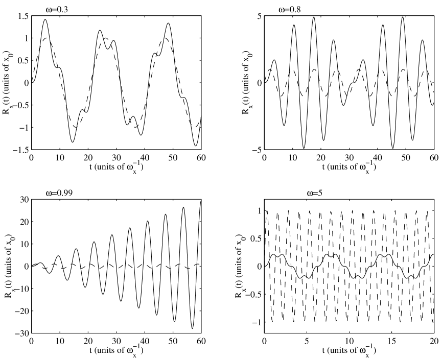
FIG. 1.: $R_{x}(t)$ for a periodically shaken trap with constant trap frequency $\omega_{x}$ and four different values of the shaking frequency $\omega$. The dashed curve is the position of the center of the trap $x_{0}(t)$.

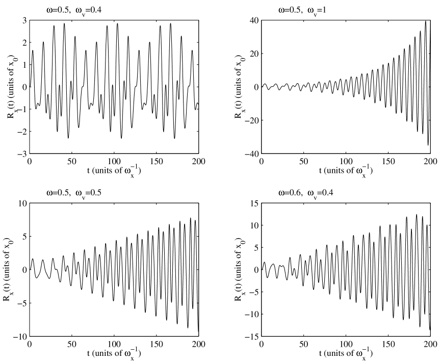
FIG. 2.: $R_{x}(t)$ for a periodically shaken trap with periodically vibrating trap frequency $\omega_{x}(t)=\omega_{x}(0)[1+0.25\sin(\omega_{v}t)]$ for different values of the shaking frequency $\omega$ and vibration frequency $\omega_{v}$.

REFERENCES

- [1] Stamper-Kurn, D. M., H.-J. Miesner, S. Inouye, M. R. Andrews, and W. Ketterle, Phys. Rev. Lett. 81, 500 (1998); Miesner, H.-J., D. M. Stamper-Kurn, M. R. Andrews, D. S. Durfee, S. Inouye, and W. Ketterle, Science 279, 1005 (1998); Inouye, S., M. R. Andrews, J. Stenger, H.-J. Miesner, D. M. Stamper-Kurn, and W. Ketterle, Nature (London) 392, 151 (1998); Jin, D. S., J. R. Ensher, M. R. Matthews, C. E. Wieman, and E. A. Cornell, Phys. Rev. Lett. 77, 420 (1996); Jin, D. S., M. R. Matthews, J. R. Ensher, C. E. Wieman, and E. A. Cornell, Phys. Rev. Lett. 78, 764 (1997); Mewes, M.-O., M. R. Andrews, N. J. van Druten, D. M. Kurn, D. S. Durfee, C. G. Townsend, and W. Ketterle, Phys. Rev. Lett. 77, 988 (1996).
- [2] S. A. Morgan, R. J. Ballagh and K. Burnett, Phys. Rev. A 53, 4338 (1997).
- [3] F. Dalfovo et al., Rev. Mod. Phys. 71, 463 (1999).
- [4] Yu. Kagan, E.L. Surkov, and G.V. Shlyapnikov, Phys. Rev. A 54, R1753 (1996); 55, R18 (1997).
- [5] Y. Castin and R. Dum, Phys. Rev. Lett. 77, 5315 (1996); 79, 3553 (1997).
- [6] W. Kohn, Phys. Rev. 143, 1242 (1961).
- [7] J. F. Dobson, Phys. Rev. Lett. 73, 2244 (1994).
- [8] E. J. Heller, J. Chem. Phys. 62, 1544 (1975).
- [9] M. Trippenbach, Y. B. Band, M. Edwards, M. Doery, and P. S. Julienne, J. Phys. B33, 47 (2000).
- [10] E. W. Hagley, L. Deng, M. Kozuma, M. Trippenbach, Y.B. Band, M. Edwards, M. Doery, P.S. Julienne, K. Helmerson, S.L. Rolston, and W.D. Phillips, Phys. Rev. Lett. 83, 3112 (1999).
- [11] M. Abramowitz and I. A. Stegun, Handbook of Mathematical Functions, (Dover, NY, 1972). See also, E.J. Heller, J.L. Ozment and D.W. Pratt, J. Chem. Phys. 88, 2169 (1988).
- [12] M. Kozuma, L. Deng, E. Hagley, J. Wen, R. Lutwak, K. Helmerson, S.L. Rolston, and W.D. Phillips, Phys. Rev. Lett.82, 871 (1999).
- [13] J. Stenger, S. Inouye, A.P. Chikkatur, D.M. Stamper–Kurn, D.E. Pritchard, and W. Ketterle, Phys. Rev. Lett.82, 4569 (1999).