Metal Nanowires: Quantum Transport, Cohesion, and Stability

Abstract

Metal nanowires exhibit a number of interesting properties: their electrical conductance is quantized, their shot-noise is suppressed by the Pauli principle, and they are remarkably strong and stable. We show that many of these properties can be understood quantitatively using a nanoscale generalization of the free-electron model. Possible technological applications of nanowires are also discussed.

Subject classification: 05.45.Mt; 47.20.Dr; 68.66.La; 73.63.Rt

1 Introduction

Metal nanowires represent nature’s ultimate limit of conductors down to a single atom in thickness. In the past eight years, experimental research on metal nanowires has burgeoned [1-13]. The simplest model of a metal is the free-electron model [14], which already describes many bulk properties of simple monovalent metals semiquantitatively. In this article, we discuss our generalization of the free-electron model to describe nanoscale conductors [15-22].

A remarkable feature of metal nanowires is the fact that they are stable at all. Fig. 1 shows electron micrographs by Kondo and Takayanagi [5] illustrating the formation of a gold nanowire. Under electron beam irradiation, the wire becomes ever thinner, until it is but four atoms in diameter. Almost all of the atoms are at the surface, with small coordination numbers. The surface energy of such a structure is enormous, yet it is observed to form spontaneously, and to persist almost indefinitely. Even wires one atom thick are found to be remarkably stable [8, 9, 13]. Naively, such structures might be expected to break apart into clusters due to surface tension [23], but we find that electron-shell effects can stabilize arbitrarily long nanowires [22].

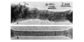
Figure 1: Transmission electron micrographs showing the formation of a gold nanowire [5] (image courtesy of Y. Kondo): (a) an image of Au(001) film with closely spaced nanoholes, the initial stage of the nanowire; (b) a nanowire four atoms in diameter, resulting from further electron-beam irradiation.

A crucial clue to understanding the physics of metal nanowires is the observed correlation between their electrical and mechanical properties. In a seminal experiment [3] carried out in 1995, Rubio, Agraït and Vieira simultaneously measured the electrical conductance and cohesive force of an atomic-scale gold wire as it formed and ruptured (see Fig. 2, left panel). They observed steps of order $G_{0}=2e^{2}/h$ in the conductance, which were synchronized with a sawtooth structure with an amplitude of order 1nN in the force. Similar results were obtained independently by Stalder and Dürig [4]. Note that the tensile strength of the nanowire in the final stages before rupture exceeds that of macroscopic gold by a factor of 20, and is of the same order of magnitude as the theoretical value in the absence of dislocations [3]. This is consistent with the recent finding of Rodrigues, Fuhrer, and Ugarte that such nanowires are, in fact, typically free of defects in their central region [13].

The standard description of nanoscale cohesion, pioneered by Landman and coworkers [24], is via molecular dynamics simulations [24, 25, 26], which utilize short-ranged interatomic potentials suitable to describe the bulk properties of metals. However, such an approach appears problematic when applied to metal nanowires, in which electron-shell effects [11] due to the transverse confinement are likely to be important. On the other hand, atomistic quantum calculations [27] using, e.g., the local-density approximation, are restricted to such small systems that their results can not really be disentangled from finite-size effects [20]. An alternative approach, developed by our group, is to replace the discrete ionic coordinates by a coarse-grained jellium background, in order to be able to treat the electronic degrees of freedom correctly. We have argued [15] that an atomic-scale contact between two pieces of metal can be thought of as a waveguide for conduction electrons (which are responsible for both electrical conduction and cohesion in simple metals): Each quantized mode transmitted through the contact contributes $2e^{2}/h$ to its conductance and a force of order $\varepsilon_{F}/\lambda_{F}$ (roughly 1nN) to its cohesion, where $\lambda_{F}$ is the de Broglie wavelength of an electron at the Fermi energy $\varepsilon_{F}$ (see Fig. 2, right panel). To my knowledge, our approach is the only one in which the observed correlations between the cohesive and conducting properties of metal nanowires have been explained within a single theoretical model.

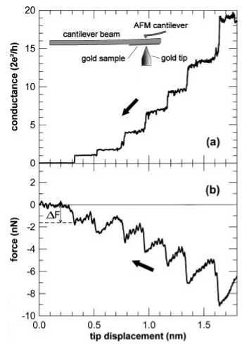
Figure 2: Left: Measured electrical conductance and cohesive force of a gold nanowire [3] (image courtesy of N. Agraït). Right: Calculated conductance and force of a metal nanowire, modeled as a constriction in a free-electron gas with hard walls [15]. Note that $\varepsilon_{F}/\lambda_{F}\simeq 1.7\mbox{nN}$ in gold.

The paper is organized as follows: The free-electron model of nanoscale conductors is introduced in the next section, followed by a discussion of quantum transport, including the effect of realistic contacts to the nanowire. Nanoscale cohesion is then analyzed within our model, followed by a discussion of the remarkable stability of nanowires. The paper concludes with some comments about the technological promise of metal nanowires.

2 Free-electron model

We investigate the simplest possible model [15, 16] for a metal nanowire: a free (conduction) electron gas confined within the wire by Dirichlet boundary conditions. A nanowire is an open quantum system, and so is treated most naturally in terms of the electronic scattering matrix $S$. The Landauer formula [28] expressing the electrical conductance in terms of the submatrix $S_{12}$ describing transmission through the wire is

$$G=\frac{2e^{2}}{h}\int d\varepsilon\frac{-\partial f(\varepsilon)}{\partial\varepsilon}\mbox{Tr}\left\{S_{12}^{\dagger}(\varepsilon)S_{12}(\varepsilon)\right\}\stackrel{{\scriptstyle T\rightarrow 0}}{{=}}\frac{2e^{2}}{h}\sum_{n}T_{n}(\varepsilon_{F}),$$ (1)

where $f(\varepsilon)$ is the Fermi-Dirac distribution function and the transmission probabilities $\{T_{n}\}$ are the eigenvalues of $S_{12}^{\dagger}S_{12}$. The conductance of a metal nanocontact was calculated exactly in this model by Torres et al. [29]. The appropriate thermodynamic potential to describe the energetics of such an open system is the grand canonical potential $\Omega$:

$$\Omega=-\frac{1}{\beta}\int d\varepsilon\,g(\varepsilon)\ln\left(1+e^{-\beta(\varepsilon-\mu)}\right)\stackrel{{\scriptstyle T\rightarrow 0}}{{=}}\int_{0}^{\varepsilon_{F}}d\varepsilon\,g(\varepsilon)(\varepsilon-\varepsilon_{F}),$$ (2)

where $\beta$ is the inverse temperature, $\mu$ is the chemical potential of electrons injected into the nanowire from the macroscopic electrodes, and $g(\varepsilon)$ is the electronic density of states (DOS) of the nanowire. The DOS of an open system may be expressed in terms of the scattering matrix as [30]

$$g(\varepsilon)=\frac{1}{2\pi i}\mbox{Tr}\left\{S^{\dagger}(\varepsilon)\frac{\partial S}{\partial\varepsilon}-\mbox{H.c.}\right\}.$$ (3)

This formula is also known as the Wigner delay. Thus, once the electronic scattering problem for the nanowire is solved, both transport and energetic quantities can be readily calculated [15, 16, 17]. Electron-electron interactions can be included at the mean-field level in this model in a straightforward way [16, 19, 21], but do not alter our main conclusions.

3 Quantum Transport

Evaluating the transmission probabilities $\{T_{n}\}$ in the WKB approximation for an axially-symmetric nanowire [15], the conductance calculated from Eq. (1) is shown in the upper-right panel of Fig. 2. Plateaus in the conductance at integer multiples of $G_{0}$ are evident, with some rounding of the steps due to tunneling. Some integers are absent, reflecting the degeneracies associated with axial symmetry [2, 29].

Conductance steps of size $G_{0}$ were first observed in quantum point contacts (QPCs) fabricated in semiconductor heterostructures [28] and are a rather universal phenomenon in metal nanowires [1-4], even being found in contacts formed in liquid metals [6]. The precision of conductance quantization in metal nanowires is poorer than that in semiconductor QPCs due to their inherently rough structure on the scale of the Fermi wavelength $\lambda_{F}$, which causes backscattering [17], and due to the imperfect hybridization of the atomic orbitals in the contact, especially for multivalent atoms [7]. For this reason, a statistical analysis of data for a large number of contacts is often made [1, 2, 6, 10, 11], resulting in a conductance histogram [see Fig. 3(a)].

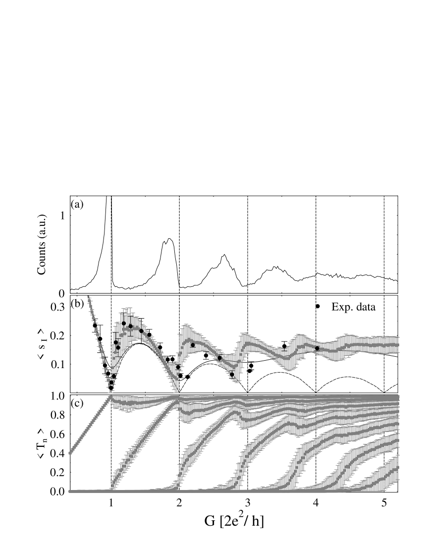
Figure 3: (a) Calculated conductance histogram [17]; (b) calculated mean shot noise $\left<s_{I}\right>$ (grey squares [18]), together with experimental data from Ref. [10] (black circles); (c) mean transmission probabilities $\left<T_{n}\right>$ [18]. The error bars indicate the standard deviations of the numerical results over the ensemble and the experimental errors, respectively.

To model quantum transport in gold nanowires, where there are no “missing integers” in the conductance histogram [1, 6, 10], geometries without axial symmetry were chosen, and weak disorder, corresponding to a mean-free path $k_{F}\ell=270$, was included both in the nanowire and in the electrodes neighboring it [17]. The transmission probabilities were calculated by solving Schrödinger’s equation using a recursive Green’s function algorithm [17]. Averaging over different contact shapes and impurity configurations, we obtained the histogram shown in Fig. 3(a), which is very similar to typical experimental histograms for gold [1, 6, 10]. The effect of disorder is twofold [17]: the conductance peaks are shifted downward due to backscattering, and the peaks are broadened due to universal conductance fluctuations, filtered by the nanowire.

Recently, additional information on quantum transport in metal nanowires has been obtained from experiments on shot noise [10]. Shot noise is the term used to describe the temporal fluctuations of electric current arising from the discreteness of the electric charge $e$. In 1918, Schottky showed that if the arrival times of charge carriers are uncorrelated, the shot-noise spectral power $P_{I}=2eI$, where $I$ is the time-average current. However, in a quantum conductor with a finite number of transmitted modes, the shot noise is suppressed below the Schottky value due to anticorrelations induced by Fermi-Dirac statistics. The suppression factor at zero temperature is given by [10]

$$s_{I}=\frac{P_{I}}{2eI}=\frac{\sum_{n}T_{n}(1-T_{n})}{\sum_{n}T_{n}}.$$ (4)

Fig. 3(b) shows the measured shot noise (solid circles [10]) of gold nanowires as a function of their conductance. The pronounced suppression of $s_{I}$ for wires with conductances near integer multiples of $G_{0}$ reveals unambiguously the quantized nature of the electronic transport. We computed [18] the mean and standard deviation of $s_{I}$ and $T_{n}$ as functions of $G$ (grey squares in Fig. 3) from the numerical data used to generate the conductance histogram in Fig. 3(a). The agreement of the experimental results for particular contacts and the calculated distribution of $s_{I}$ shown in Fig. 3(b) is extremely good: 67% of the experimental points lie within one standard deviation of $\langle s_{I}\rangle$ and 89% lie within two standard deviations. It should be emphasized that no attempt has been made to fit the shot-noise data; the numerical data of Ref. [17], where the length of the contact and the strength of the disorder were chosen to model experimental conductance histograms for gold, have simply been reanalyzed to calculate $\langle s_{I}\rangle$. The 97% suppression of shot noise for nanowires with a single quantum of conductance (i.e., wires one atom thick) suggests that such wires could be useful for low-temperature/low-noise applications, such as quantum computing.

4 Metallic nanocohesion

The cohesive force of the nanowire is $F=-\partial\Omega/\partial L$, where $L$ is the length of the nanowire. We assume that the volume per atom is conserved under elongation (ideal plastic deformation), so that the deformation occurs at constant volume (for alternative constraints, see Refs. [19, 21]). While the conductance is determined by the transmission probabilities, Eqs. (2) and (3) indicate that the energetics of a nanowire are determined by the scattering phase shifts. Evaluating the phase shifts in the WKB approximation, performing the energy integral in Eq. (2) at $T=0$, and taking the derivative with respect to elongation [15], one finds the force shown in the lower-right panel of Fig. 2. The correlations between the force and conductance are striking: as the wire is elongated and its diameter decreases, $|F|$ increases along a conductance plateau, but decreases sharply when the conductance drops. Each transmitted mode acts like a delocalized metallic bond, which can be stretched and broken.

The calculated force is remarkably similar, both quantitatively and qualitatively, to the measured force for gold nanowires, shown in the lower-left panel of Fig. 2. Inserting the value $\varepsilon_{F}/\lambda_{F}\simeq 1.7\mbox{nN}$ for gold, we see that both the overall scale of the force for a given value of the conductance and the heights of the last two force oscillations are in quantitative agreement with the experimental data. One discrepancy is that the jumps in both force and conductance are less abrupt than in the experimental curves, possibly because we considered only geometries that change continuously with elongation.

In order to separate out the mesoscopic sawtooth structure in the force, associated with the opening of individual conductance channels, from the overall (macroscopic) trend of the contact to become stronger as its diameter increases, it is useful to perform a systematic semiclassical expansion [31, 32] of the DOS, $g(\varepsilon)=\bar{g}(\varepsilon)+\delta g(\varepsilon)$, where $\bar{g}$ is a smooth average term, referred to as the Weyl contribution, and $\delta g(\varepsilon)$ is an oscillatory term, whose average is zero. For the free electron model with Dirichlet boundary conditions, the Weyl term is [32]

$$\bar{g}(\varepsilon)=\varepsilon^{-1}\left(\frac{k^{3}V}{2\pi^{2}}-\frac{k^{2}A}{8\pi}+\frac{k\,C}{6\pi^{2}}\right),$$ (5)

where $k=\sqrt{2m\varepsilon}/\hbar$, $V$ is the volume of the wire, $A$ its surface area, and $C$ the integrated mean curvature of its surface. The oscillatory contribution $\delta g(\varepsilon)$ to the DOS may be approximated as a Feynman sum over classical periodic orbits à la Gutzwiller [31, 32]:

$$\delta g(\varepsilon)=\sum_{\nu}A_{\nu}\cos\left(\frac{S_{\nu}(\varepsilon)}{\hbar}+\theta_{\nu}\right),$$ (6)

where $S_{\nu}$ is the classical action of a periodic orbit, $\theta_{\nu}$ is a phase shift determined by the singular points along the classical trajectory, and $A_{\nu}$ is an amplitude depending on the stability, symmetry, and period of the orbit. Using $\bar{g}(\varepsilon)$ in Eq. (2), one can derive a Sharvin-like formula for the force

$$F=\bar{F}+\delta F,\qquad\bar{F}=-\frac{\varepsilon_{F}}{\lambda_{F}}\left(\frac{\pi k_{F}D}{16}-\frac{4}{9}\right).$$ (7)

The first term in $\bar{F}$ is the surface tension. The oscillatory mesoscopic correction $\delta F$ may be calculated with the aid of Eq. (6). Under reasonable assumptions about the geometry, it can be shown [19] that the amplitude of the force oscillations is universal:

$$\mbox{rms}\,\delta F=0.58621\,\varepsilon_{F}/\lambda_{F}.$$ (8)

In more realistic models including electron-electron interactions [16, 19, 21] and self-consistent confining potentials [33], the surface tension is typically reduced compared to Eq. (7), but the force oscillations are essentially the same as in the free-electron model.

5 Stability of Nanowires

Figure 4: Density of states $g(\varepsilon_{F})$ of a cylindrical wire (upper diagram) and zero temperature stability coefficient $\alpha$ (lower diagram) versus the radius $R_{0}$ of the unperturbed wire. The wavevector of the perturbation is $qR_{0}=1$. Dashed curve: Weyl contribution to $\alpha$.

A cylindrical body longer than its circumference is unstable to breakup under surface tension [23], a phenomenon known as the Rayleigh instability. How then to explain the durability of long gold nanowires [c.f. Fig. 1(b)], the thinnest of which have been shown [12] to be almost perfectly cylindrical in shape? The key is the quantum corrections [22] to the classical stability coefficients.

Only axially-symmetric deformations can lower the surface energy of a cylindrical object, and thus lead to an instability [23]. Any such deformation may be written as a Fourier series

$$R(z)=R_{0}+\int_{-\infty}^{\infty}dq\,b(q)e^{iqz},$$ (9)

where $R(z)$ is the radius of the wire at $z$, $R_{0}$ is the radius of the unperturbed cylinder, and $b(q)$ is a complex perturbation coefficient. Using Eqs. (5) and (6) in Eq. (2), one obtains the following expansion [22]

$$\Omega[b]=\Omega[0]+\int_{0}^{\infty}\!\!dq\,\alpha(q)|b(q)|^{2}+{\cal{O}}(b^{3}),$$ (10)

where the stability coefficient $\alpha(q)$ depends implicitly on $R_{0}$ and $T$. The change in the grand canonical potential is of second order in $b$ and contributions from deformations with different $q$ decouple. If $\alpha(q)$ is negative for any value of $q$, then $\Omega$ decreases under the deformation and the wire is unstable.

Let us first discuss the stability of a nanowire at zero temperature. Fig. 4 shows the stability coefficient (lower diagram) and DOS (upper diagram) at the classical stability threshold $qR_{0}=1$ as a function of $R_{0}$. For a straight wire, the transverse motion is quantized, and the DOS consists of a sequence of sharp peaks associated with the opening of each successive subband. $\alpha$ has sharp negative peaks—indicating strong instabilities—at the subband thresholds, where the density of states is sharply peaked. Under surface tension and curvature energy alone (dashed curve in Fig. 4), the wire would be slightly unstable at the critical wavevector $qR_{0}=1$, since the curvature term is negative. However, the quantum correction is positive in the regions between the thresholds to open new subbands, thus stabilizing the wire. Since the oscillatory contribution to $\alpha$ is independent of $q$, we find that regions of stability persist for arbitrarilly long wavelength perturbations, indicating that an infinitely long cylindrical wire is a true metastable state if the radius lies in one of the windows of stability.

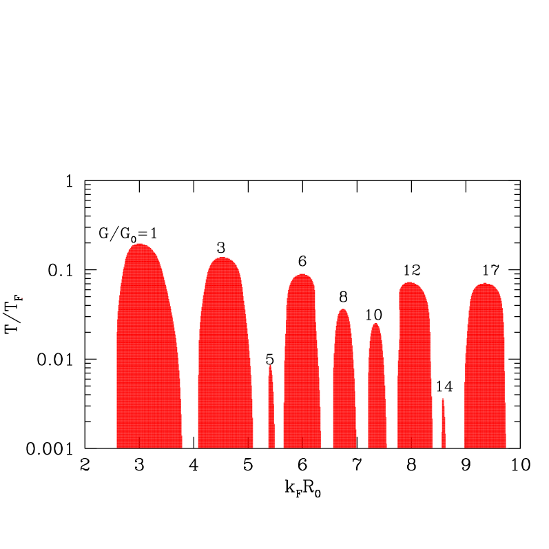
Figure 5: Stability of metal nanowires as a function of radius and temperature. Shaded regions indicate stability with respect to small perturbations; unshaded regions denote unstable configurations. Here $T_{F}$ is the Fermi temperature and $R_{0}$ is the mean radius of the wire. The quantized conductance values of the stable wires are indicated.

With these results, we can construct a stability diagram for metal nanowires (see Fig. 5). In the semiclassical approximation, $d\alpha/dq>0$ always, so the stability of the wire is determined by the sign of $\alpha(q=0)$. $\alpha(0)$ is a function of two dimensionless parameters, $k_{F}R_{0}$ and $T/T_{F}$. Regions where $\alpha(0)>0$ are shaded dark in Fig. 5, while regions where $\alpha(0)<0$ are unshaded. The stable regions persist up to extremely high temperatures for several quantized conductance values (recall that $T_{F}>10^{4}\mbox{K}$ for metals), indicating that electron-shell effects may stabilize nanowires even for temperatures well above the bulk melting temperature. It is important to point out that if a more realistic value of the surface tension [19, 21, 33] were used, the stability boundaries would be pushed to even higher temperatures. Thus the astounding stability properties shown in Fig. 5 are a very robust prediction of the jellium model.

6 Conclusions

Wires formed from chains of individual metal atoms have a number of properties which make them promising for nanotechnology: They are very strong, able to support tensions up to $\varepsilon_{F}/\lambda_{F}\approx 1\mbox{nN}$. Contrary to naive expectations, they are extremely stable, despite their large surface to volume ratio. They are nearly-ideal one-dimensional conductors, and exhibit dramatically-reduced shot noise. One potential application of metal nanowires is for integrated-circuit interconnects, due to their high conductance and structural robustness. The quantum suppression of shot noise in nanowires may also make them useful for low-temperature/low-noise applications, such as quantum computing.

AcknowledgementsI am indebted to Jérôme Bürki, Frank Kassubek, and Chang-hua Zhang, the students and postdocs without whom much of this research would have been impossible. I also wish to thank Dionys Baeriswyl, Raymond Goldstein, Hermann Grabert, and Xenophon Zotos for their valuable contributions. This research was supported by NSF grant DMR0072703 and by an award from Research Corporation.

References

- [1] L. Olesen et al., Phys. Rev. Lett. 72, 2251 (1994); Phys. Rev. Lett. 74, 2147 (1994).
- [2] J. M. Krans et al., Nature 375, 767 (1995).
- [3] G. Rubio, N. Agraït, and S. Vieira, Phys. Rev. Lett. 76, 2302 (1996).
- [4] A. Stalder and U. Dürig, Appl. Phys. Lett. 68, 637 (1996).
- [5] Y. Kondo and K. Takayanagi, Phys. Rev. Lett. 79, 3455 (1997).
- [6] J. L. Costa-Krämer et al., Phys. Rev. B 55, 5416 (1997).
- [7] E. Scheer et al., Nature 394, 154 (1998).
- [8] H. Ohnishi, Y. Kondo, and K. Takayanagi, Nature 395, 780 (1999).
- [9] A. I. Yanson et al., Nature 395, 783 (1999).
- [10] H. E. van den Brom and J. M. van Ruitenbeek, Phys. Rev. Lett. 82, 1526 (1999).
- [11] A. I. Yanson, I. K. Yanson, and J. M. van Ruitenbeek, Nature 400, 144 (1999); Phys. Rev. Lett. 84, 5832 (2000).
- [12] Y. Kondo and K. Takayanagi, Science 289, 606 (2000).
- [13] V. Rodrigues, T. Fuhrer, and D. Ugarte, Phys. Rev. Lett. 85, 4124 (2000); V. Rodrigues and D. Ugarte, Phys. Rev. B 63, 073405 (2001).
- [14] N. W. Ashcroft and N. D. Mermin, Solid State Physics, Saunders College Publishing, New York, 1976 (pp. 29-55).
- [15] C. A. Stafford, D. Baeriswyl, and J. Bürki, Phys. Rev. Lett. 79, 2863 (1997).
- [16] F. Kassubek, C. A. Stafford, and H. Grabert, Phys. Rev. B 59, 7560 (1999).
- [17] J. Bürki, C. A. Stafford, X. Zotos, and D. Baeriswyl, Phys. Rev. B 60, 5000 (1999); Phys. Rev. B 62, 2956 (2000).
- [18] J. Bürki and C. A. Stafford, Phys. Rev. Lett. 83, 3342 (1999).
- [19] C. A. Stafford, F. Kassubek, J. Bürki, and H. Grabert, Phys. Rev. Lett. 83, 4836 (1999); F. Kassubek, C. A. Stafford, and H. Grabert, Physica B 280, 438 (2000).
- [20] C. A. Stafford, J. Bürki, and D. Baeriswyl, Phys. Rev. Lett. 84, 2548 (2000).
- [21] C. A. Stafford et al., in: Quantum Physics at the Mesoscopic Scale, D. C. Glattli, M. Sanquer, and J. Trân Thanh Vân eds., EDP Sciences, Les Ulis (France), 2000 (p. 49).
- [22] F. Kassubek, C. A. Stafford, H. Grabert, and R. E. Goldstein, Nonlinearity 14, 167 (2001); C. A. Stafford, F. Kassubek, and H. Grabert, Adv. Solid State Phys. 41, 497 (2001).
- [23] S. Chandrasekhar, Hydrodynamic and Hydromagnetic Stability, Dover, New York, 1981 (pp. 515-74).
- [24] U. Landman, W. D. Luedtke, N. A. Burnham, and R. J. Colton, Science 248, 454 (1990).
- [25] T. N. Todorov and A. P. Sutton, Phys. Rev. B 54, R14234 (1996).
- [26] M. R. Sørensen, M. Brandbyge, and K. W. Jacobsen, Phys. Rev. B 57, 3283 (1998).
- [27] H. Hakkinen and M. Manninen, Europhys. Lett. 44, 80 (1998); A. Nakamura, M. Brandbyge, L. B. Hansen, and K. W. Jacobsen, Phys. Rev. Lett. 82, 1538 (1999).
- [28] S. Datta, Electronic Transport in Mesoscopic Systems, Cambridge University Press, 1995 (pp. 48-170).
- [29] J. A. Torres, J. I. Pascual, and J. J. Sáenz, Phys. Rev. B 49, 16581 (1994).
- [30] R. Dashen, S.-K. Ma, and H. J. Bernstein, Phys. Rev. 187, 345 (1969).
- [31] M. C. Gutzwiller, Chaos in Classical and Quantum Mechanics, Springer, New York, 1990.
- [32] M. Brack and R. K. Bhaduri, Semiclassical Physics, Addison-Wesley, Reading, MA, 1997.
- [33] C. Yannouleas, E. N. Bogachek, and U. Landman, Phys. Rev. B 57, 4872 (1998).