Theory of the dc Magnetotransport in Laterally Modulated Quantum Hall Systems Near Filling $\displaystyle\ {\cal V}=\frac{1}{2}$

Abstract

A quasiclassical theory for dc magnetotransport in a modulated quantum Hall system near filling factor $\nu=\frac{1}{2}$ is presented. A weak one-dimensional electrostatic potential acts on the two-dimensional electron gas. Closed form analytic expressions are obtained for the resistivity $\rho_{\perp}$ corresponding to a current at right angles to the direction of the modulation lines as well as a smaller component $\rho_{||}$ for a current along the direction of the modulation lines. It is shown that both resistivity components are affected by the presence of the modulation. Numerical results are presented for $\rho_{\perp}$ and $\rho_{||}$ and show reasonable agreement with the results of recent experiments.

I 1. Introduction and Background

It is well known that the transport properties of a two-dimensional electron gas (2DEG) in high magnetic fields providing a half filling of the lowest Landau level ($\nu=1/2$) are well described by the theory of Halperin, Lee and Read (HLR) one ; two which corresponds to a physical picture in which electrons are decorated by attached quantum flux tubes. These are the relevant quasiparticles of the system – so-called composite fermions (CFs). The CFs are spinless fermionic quasiparticles with charge $-e$ which move in a reduced effective magnetic field $B_{eff}=B-4\pi\hbar nc/e$, where $n$ is the electron sheet density. At $\nu=1/2$, the CFs form a Fermi sea and exhibit a Fermi surface (FS). For the homogeneous 2DEG, the FS of the CFs is a circle of radius $p_{F}=\sqrt{4\pi n\hbar^{2}}$ in quasimomentum space.

According to the theory of HLR, the resistivity tensor of the 2DEG is given by $\tensor{\rho}=\tensor{\rho}_{cf}+\tensor{\rho}_{cs}$, where $\tensor{\rho}_{cf}$ is the contribution from CFs whereas $\tensor{\rho}_{cs}$ arises from the fictitious effective magnetic field in the Chern-Simons formulation of the theory. Here, $\tensor{\rho}_{cs}$ has only off-diagonal elements. Therefore, the diagonal elements of the resistivity tensor of the 2DEG are the same as those for the CF resistivity tensor $\tensor{\rho}_{cf}=\tensor{\sigma}_{cf}^{-1}$, where $\tensor{\sigma}_{cf}$ is the CF conductivity tensor.

Some interesting features of the magnetoresistivity near $\nu=1/2$ have been reported in the transport experiments of a 2DEG whose density is modulated by a weak one-dimensional electrostatic potential. This includes a well-defined minimum at $\nu=1/2$ in the resistivity $\rho_{\perp}$ corresponding to a current at right angles to the direction of the modulation lines three ; four as well as a smaller component $\rho_{||}$ with a maximum at $\nu=1/2$ for a current along the lines of the modulation four . In addition, oscillations in these two components of the resistivity were observed close to filling factor $\nu=1/2$. Previous theories for dc magnetotransport in modulated quantum Hall systems near one half filling based on the Boltzmann transport equation for the CF distribution function five ; six ; seven are succesfull in accounting for the minimum in the magnetoresistivity $\rho_{\perp}.$ However, these theories, as well as semiclassical studies of dc magnetotransport properties of modulated 2DEG at low magnetic field eight ; nine ; ten ; eleven , fail to explain the magnetic field dependence of $\rho_{||}.$ Up to present the effect of modulations on $\rho_{||}$ was treated as a pure quantum effect which cannot be described within semiclassical calculations, although it remains exhibited within that range of magnetic fields where the semiclassical approach could be applied twelve ; thirteen ; fourteen ; fifteen .

We think that the existing theory is mistaken at this point, and the magnetic field dependence of both resistivity components near $\nu=1/2$ is dominated with similar mechanism and could be analyzed within a semiclassical approximation. This can be shown if we adopt a correct procedure of averaging of CF response functions over the period of modulations sixteen ; seventeen which gives semiclassical analogs for the response functions obtained as a result of quantum mechanical calculations. The proposed procedure differs from that used in the existing semiclassical theories eight ; nine ; ten ; eleven and provides different results for transport coefficients of a modulated 2DEG. In contrast with the corresponding conclusions of the earlier works, our results for the both components of magnetoresistivity tensor are consistent with those obtained as a semiclassical limit of quantum mechanical calculations (see e.g. thirteen ). They also demonstrate a better agreement with experiments on a dc magnetotransport in a modulated 2DEG in low magnetic fields.

In the main body of the paper we use a simplified semiquantitative approach, resembling that used in earlier works of Beenakker eight and Gerhardts nine . In the experiments of Ref.4 the mean free path $l$ of the CFs is larger than their cyclotron radius $R$ but smaller or of the same order as the period of modulations $\lambda.$ In this ”local” regime $R,l<\lambda$ this method of calculations gives reasonably good approximation for the transport coefficients we seek.

In the Appendix, we present calculations of the magnetoresistivity components based on the transport Boltzmann equation within a relaxation time approximation. The results of this analysis corroborate reasonably with the semiquantitative approach developed in the main body of the paper.

II 2. General Formulation of the Problem

We now consider a sinusoidal density modulation with a single harmonic of period $\lambda=2\pi/g$ along the $y$ direction and given by $\Delta n({\bf r})=\Delta n\sin(gy)$. This density modulation influences the CF system through the appearance of an additional inhomogeneous magnetic field $\Delta B({\bf r})=-4\pi\hbar c\Delta n(y)/e$, which is proportional to the density modulation $\Delta n(y)$ as well as through the external modulating electric field. Following Ref. seven , we parameterize the electric potential screened by the 2DEG as

$${U(y)=\frac{\Delta n}{n}E_{F}\frac{\sin(gy)}{e}},$$

where $E_{F}$ is the Fermi energy of the unmodulated CF system.

Our starting point is the Lorentz force equations describing the CF motion along the cyclotron orbits

$$\frac{dp_{x}}{dt} = -\frac{e}{c}B(y)v_{y};$$

$$\frac{dp_{y}}{dt} = \frac{e}{c}B(y)v_{x}+e\frac{dU(y)}{dy}\ ,$$ (1)

where $p_{x},p_{y}$ and $v_{x},v_{y}$ are the components of the quasimomentum and velocity of the CF and $B(y)=B_{eff}-4\pi\hbar\Delta n(y)c/e$.

For weak modulations, $\Delta n/n\ll 1$, we may assume that inhomogeneous terms in Eq. (1) are small for all values of $B_{eff}$ except when the filling factor is close to $\nu=1/2$, where $B_{eff}\to 0$. In this limit, we can write the CF velocity as ${\bf v}={\bf v}_{0}+\delta{\bf v}$, where ${\bf v}_{0}$ is the uniform field velocity and the correction $\delta{\bf v}$ is due to the density modulation. For a circular CF–FS, we have $v_{x0}=v_{F}\cos\Omega t,\ \ v_{y0}=v_{F}\sin\Omega t,\ \ \Delta n(y)\approx\Delta n\sin(gY\\ -gR\cos\Omega t)$, where $\Omega$ is the cyclotron frequency, $v_{F}$ is the Fermi velocity for CFs, $R=v_{F}/\Omega$ is the cyclotron radius, and $Y$ is the $y$ coordinate of the guiding center. Substituting these results for ${\bf v}$ and $\Delta n(y)$ into Eq. (1) and keeping only the terms to first order in the perturbation, we obtain

$$\frac{d(\delta v_{x})}{dt}=-\Omega\delta v_{y}-\frac{\Delta B}{B_{eff}}\Omega v_{F}\sin(\Omega t)\sin(gY-gR\cos(\Omega t))\ ,$$ (2)

$$\frac{d(\delta v_{y})}{dt} = \Omega\delta v_{x}+\frac{\Delta B}{B_{eff}}\Omega v_{F}\cos(\Omega t)\sin(gY-gR\cos(\Omega t))$$ (3)

$$+ \frac{1}{2}\frac{\Delta n}{n}v_{F}^{2}g\cos(gY-gR\cos(\Omega t))\ .$$

Apart from its effect for a modulation potential in a low magnetic field, it has been shown to order $\Delta n/n$ that the modulating potential $U(y)$ gives rise to spatially inhomogeneous corrections to the chemical potential and Fermi velocity of the quasiparticles as well as their scattering rates ten . For the CF system, $\Delta n/n$ may be treated as a much smaller parameter than $\Delta B/B_{eff}$. Therefore, we neglect the corrections to the CF Fermi velocity in Eqs. (12) and (13) as well as the corrections to the relaxation time.

We would like to point out that when some effects of electric modulation are neglected, one misses the possibility of describing an asymmetry in the shape near the minimum of $\rho_{\perp}$ near $B_{eff}=0$ which was observed in the experiments three ; four . It was shown by Zwerschke and Gerhardts seven that the small asymmetry of $\rho_{\perp}$ as a function of $B_{eff}$ near $B_{eff}=0$ originates from the effect of interference of the applied electric modulations and induced magnetic modulations. We believe that the observed asymmetry four in the shape near the maximum in $\rho_{||}$ is also due to the same reason. However, we do not analyze this effect here to avoid extra complications arising from additional calculations.

To lowest order in the modulating field, the corrections $\delta v_{x}$ and $\delta v_{y}$ are periodic over the unperturbed cyclotron orbit, as was used in Ref. nine . With this assumption, we calculate the averages of Eqs. (2) and (3) over the cyclotron orbit. After a straightforward calculation, we obtain the following results for the components $V_{x}$ and $V_{y}$ of the velocity of the guiding center

$$V_{x}(Y) = \frac{1}{2\pi}\int_{0}^{2\pi}d\psi\ \delta v_{x}(Y,\psi)=v_{F}\cos(gY)$$ (4)

$$\times \left[\frac{\Delta B}{B_{eff}}J_{1}(gR)-\frac{1}{2}gR\frac{\Delta n}{n}J_{0}(gR)\right],$$

$$V_{y}(Y) = \frac{1}{2\pi}\int_{0}^{2\pi}d\psi\ \delta v_{y}(Y,\psi)=0\ ,$$ (5)

where $\psi=\Omega t$, and $J_{0}(gR)$, $J_{1}(gR)$ are Bessel functions of the first kind. We now calculate the CF conductivity by assuming, as before seventeen , that $v_{x}(Y)=v_{x0}+V_{x}(Y)$ and that the cyclotron frequency $\Omega$ can be replaced by $\Omega(Y)=\Omega+\Delta\Omega(Y)$, where $\Delta\Omega(Y)$ is the correction to the cyclotron frequency due to the inhomogeneous effective magnetic field, averaged over the cyclotron orbit,

$$\Omega(Y) = \Omega\left\{1+\frac{\Delta B}{B_{eff}}\frac{1}{2\pi}\int_{0}^{2\pi}d\psi\ \sin(gY-gR\cos\psi)\right\}$$ (6)

$$= \Omega\left\{1+\frac{\Delta B}{B_{eff}}\sin(gY)J_{0}(gR)\right\}\ .$$

Within the local limit $R<<\lambda$ the guiding center velocity (3) becomes neiligible, and the conductivity tensor $\tensor{\sigma}_{cf}(Y)$ has the Drude form with the cyclotron frequency $\Omega$ replaced by $\Omega(Y).$

We now introduce the current density of CFs, averaged over the period of the modulation,

$${\bf j}=<{\bf j}(Y)>=\frac{g}{2\pi}\int_{-\pi/g}^{\pi/g}dY\ {\bf j}(Y)\ .$$ (7)

Within the local limit ${\bf j}(Y)$ related to a driving electric field by the usual linear relation:

$${\bf j}(Y)=\tensor{\sigma}_{cf}(Y)\cdot\left({\bf E}+\Delta{\bf E}(Y)\right)$$ (8)

with ${\bf E}$ denoting the external electric field and $\Delta{\bf E}(Y)$ the inhomogeneous contribution to the total electric field due to the density modulation, averaged over the cyclotron orbit. To proceed we define the effective CF conductivity by the relation

$${\bf j}=\tensor{\sigma}_{cf}\cdot<{\bf E}+\Delta{\bf E}(Y)>.$$ (9)

When an electrostatic modulation is applied along the $y$ direction, it affects only the current along the direction of the modulation lines ten , so within the geometry chosen here, $j_{y}$ does not depend on the $y$ coordinate. This result follows from the continuity equation. Consequently, we assume that $j_{y}$ is independent of $Y$. Also, since $E_{x}$ does not depend on $Y$, we can obtain closed form analytic expressions for the effective CF conductivity tensor from Eq. (9). To get these expressions we first assume that $E_{x}=0$ and solve for the conductivity to obtain

$$\sigma_{cf}^{yy}=\left<\frac{1}{\sigma_{cf}^{yy}(Y)}\right>^{-1}\ .$$ (10)

Solving again for $E_{y}$ and assuming that $<E_{y}(Y)>=0$, we obtain

$$\sigma_{cf}^{yx}=-\sigma_{cf}^{xy}=\left<\frac{\sigma_{cf}^{yx}(Y)}{\sigma_{cf}^{yy}(Y)}\right>\left<\frac{1}{\sigma_{cf}^{yy}(Y)}\right>^{-1}\ .$$ (11)

Finally, substituting the result for $E_{y}(Y)$ into the expression for the $x$ component of Eq. (9), and making use of

$$<j_{x}(Y)>=\left<\frac{\sigma_{cf}^{xy}(Y)}{\sigma_{cf}^{yy}(Y)}\right>j_{y}\ ,$$

we obtain

$$\sigma_{cf}^{xx}=\left<\sigma_{cf}^{xx}+\frac{\sigma_{cf}^{xy}(Y)}{\sigma_{cf}^{yy}(Y)}\left(\sigma_{cf}^{yx}-\sigma_{cf}^{yx}(Y)\right)\right>\ .$$ (12)

Now we define the effective CF magnetoresistivity $\tensor{\rho}_{cf}$ as $\tensor{\sigma}_{cf}^{-1}$. The above results for the effective conductivity components are valid in the local regime, regardless of the dc magnetotransport experiments. We use this to analyze the experimental data. Assuming that the current flows along the modulation lines ($j_{y}=0$), we obtain the following result for the magnetoresistivity

$$\rho_{||}=\rho_{xx}=\left\{<\sigma_{cf}^{xx}(Y)>+\left<\frac{\sigma_{cf}^{xy}(Y)^{2}}{\sigma_{cf}^{yy}(Y)}\right>\right\}^{-1};$$ (13)

Similarly, when current is driven across the modulation lines, and $<j_{x}>=0$ we get the expression for $\rho_{\perp}$ in the form:

$$\rho_{\perp}=\rho_{yy}=\left<\frac{1}{\sigma_{cf}^{yy}(Y)}\right>-\frac{\displaystyle{\left<\frac{\sigma_{cf}^{xy}(Y)}{\sigma_{cf}^{yy}(Y)}\right>^{2}}}{\displaystyle{<\sigma_{cf}^{xx}(Y)>+\left<\frac{\sigma_{cf}^{xy}(Y)^{2}}{\sigma_{cf}^{yy}(Y)}\right>}}\ .$$ (14)

It follows from these results that in the local regime the transverse resistivity $\rho_{\perp}$ shows a positive magnetoresistance proportional to $\big{(}\Omega\tau\Delta B/B_{eff}\big{)}^{2},$ whereas the longitudinal resistivity remains unchanged at the presence of modulations and takes on its Drude value which agrees with the current theory ten .

To analyze the influence of modulations on the magnetotransport characteristics within a broader range of magnetic fields $R\stackrel{{\scriptstyle<}}{{\sim}}\lambda$ we take into account corrections to the usual Drude conductivity originating from the guiding center drift. For this purpose we now introduce the conductivity tensor $\tensor{\sigma}_{cf}(Y)$ in the form:

$$\sigma_{cf}^{\alpha\beta}(Y)=\frac{e^{2}m_{c}\tau}{2\pi\hbar^{2}}\sum_{k=-\infty}^{\infty}\frac{v_{k\alpha}(Y)v_{-k\beta}(Y)}{1+ik\Omega(Y)\tau}\ \ ,$$ (15)

where $m_{c}$ is the cyclotron mass of the CF, $\tau$ is the relaxation time, $v_{k\beta}(Y)$ denotes the Fourier series coefficients of the velocity components given by

$\displaystyle v_{kx}=\frac{v_{F}}{2}(\delta_{k,1}+\delta_{k,-1})+V_{x}(Y)\delta_{k,0}\qquad$ and
$\displaystyle v_{ky}=\frac{iv_{F}}{2}(\delta_{k,1}-\delta_{k,-1})$.

Similar expression for the ”nonlocal” conductivity was used by Gerhardts nine (see Eqs. (2.10), (2.11) of the above paper), and earlier by Beenakker eight .

Starting from the definition (15), keeping only those terms up to order $(\Delta B/B_{eff})^{2}$ and using

$$\frac{\Delta B}{B_{eff}}\Omega\tau=\frac{\Delta n}{n}\frac{p_{F}}{\hbar}\ell=\frac{\Delta n}{n}k_{F}\ell\ ,$$

we obtain the following results for the effective CF conductivity components (8)–(10):

$$\sigma_{cf}^{xx} = \frac{\sigma_{0}}{1+(\Omega\tau)^{2}}\left\{1+\frac{1}{2}\left(\frac{\Delta n}{n}k_{F}\ell\right)^{2}\frac{(\Omega\tau)^{2}}{1+(\Omega\tau)^{2}}J_{0}^{2}(gR)\right\}$$ (16)

$$+ \sigma_{0}\left(\frac{\Delta B}{B_{eff}}\right)^{2}\left(J_{1}(gR)-\frac{g}{2k_{F}}J_{0}(gR)\right)^{2},$$

$$\sigma_{cf}^{yx} = -\sigma_{cf}^{xy}$$ (17)

$$= -\frac{\sigma_{0}\Omega\tau}{1+(\Omega\tau)^{2}}\left\{1-\frac{1}{2}\left(\frac{\Delta n}{n}k_{F}\ell\right)^{2}\frac{J_{0}^{2}(gR)}{1+(\Omega\tau)^{2}}\right\},$$

$$\sigma_{cf}^{yy} = \frac{\sigma_{0}}{1+(\Omega\tau)^{2}}\left\{1-\frac{1}{2}\left(\frac{\Delta n}{n}k_{F}\ell\right)^{2}\frac{J_{0}^{2}(gR)}{1+(\Omega\tau)^{2}}\right\},$$ (18)

where, in this notation, $\sigma_{0}=ne^{2}\ell/p_{F}$ is the Drude conductivity for CFs. The last term in Eq.(16) for $\sigma_{cf}^{xx}$ shows the drift of the guiding center and represents the diffusion of CFs in the $x$ direction. This can be verified by calculating the corresponding $x$ component of the diffusion coefficient $\delta{\cal D}$. Following Ref. eight , we have

$$\delta{\cal D} = \tau<V_{x}^{2}(Y)>$$

$$= \frac{v_{F}^{2}\tau}{2}\left(\frac{\Delta B}{B_{eff}}\right)^{2}\left(J_{1}(gR)-\frac{g}{2k_{F}}J_{0}(gR)\right)^{2}.$$

Substituting Eq. (18) into the Einstein relation $\sigma_{cf}^{\alpha\beta}=Ne^{2}{\cal D}_{\alpha\beta}$, where $N$ is the density of states for CFs, we obtain the last term in Eq. (19).

Using our expressions (16)–(18) we may calculate the diagonal components of the electronic resistivity tensor from the CF conductivity tensor $\tensor{\sigma}_{cf}$ given by Eqs. (11) and (12). When the density modulation is very weak, i.e., $\displaystyle{\frac{\Delta n}{n}k_{F}\ell\ll 1}$, the corrections to the magnetoresistivity due to the density modulation are small and may be neglected. In this case, the nonuniform part of the effective magnetic field does not significantly alter the dc transport. For stronger modulation, i.e., $\displaystyle{\frac{\Delta n}{n}k_{F}\ell\sim 1}$, the resistivity components are changed considerably. Keeping only the largest contributions when $\Delta B/B_{eff}$ is treated as a small parameter, we obtain the following approximate results for the components of the electron resistivity $\rho_{\perp}=\rho_{yy}$ and $\rho_{||}=\rho_{xx}$ corresponding to current flowing perpendicular and parallel, respectively, to the modulation lines.

$$\rho_{\perp} = \frac{1}{\sigma_{0}}\left\{1+\left(\frac{\Delta n}{n}k_{F}\ell\right)^{2}\left[J_{1}^{2}(gR)+\frac{1}{2}J_{0}^{2}(gR)\right]\right\},$$

$$\rho_{||} = \frac{1}{\sigma_{0}}\left\{1-\left(\frac{\Delta n}{n}\frac{k_{F}}{g}\right)^{2}(gR)^{2}\right.$$ (21)

$$\times \left.\left[J_{1}(gR)-\frac{1}{2}\frac{g}{k_{F}}J_{0}(gR)\right]^{2}\right\}.$$

We arrived at the expressions (20), (21) for magnetoresistivities as a result of a semiquantitative analysis described above. Our analysis is a merely semiquantitative one for it employs the relation (7) in ”nonlocal” $(R\stackrel{{\scriptstyle<}}{{\sim}}\lambda)$ calculations whereas this relation is completely adequate only within the extremely local regime $(R<<\lambda).$ However, similar considerations were carried out before eight ; nine , and it was shown eight ; nine ; ten that they yield results which basically agree with those obtained with proper calculations based on the Boltzmann transport equation. Here, we also use the latter to justify our results for resistivity components (see Appendix).

It follows from Eqs. (20) and (21) that both resistivities are influenced by the one-dimensional modulation, ruling out the local limit $R<<\lambda.$ This disagrees with the results obtained in Refs. five ; six ; seven ; eight ; nine ; ten ; eleven , where it was stated that only one component of the resistivity, i.e., $\rho_{\perp}$, changes as a result of the modulation. Comparison of our theory with the existing semiclassical theories shows that the difference in the results arises from the difference in definitions of the effective magnetoresistivity. Here, we define $\tensor{\rho}_{cf}$ as $\tensor{\sigma}_{cf}^{-1}$ where $\tensor{\sigma}_{cf}$ is introduced by Eq. (9), whereas Menne and Gerhardts ten use a different definition for the effective magnetoresistivity, namely:

$$\tensor{\rho}<{\bf j}>={\bf E}.$$

In other words, we first introduce the averaged effective conductivity and then we calculate the magnetoresistivity tensor, as an inverse of the effective conductivity. This is in contrast with Refs. five ; six ; seven ; eight ; nine ; ten ; eleven where the average was carried out last eighteen .

Our point to justify the averaging procedure based on the definition (7) is that the expressions for transport coefficients obtained either with quantum mechanical or with classical calculations have to be consistent at low magnetic fields where the cyclotron quantum $\hbar\Omega$ is minute compared to the Fermi energy of the system. Quantum mechanical calculations of the magnetoconductivity twelve ; thirteen ; fourteen ; fifteen insert summation over quantum numbers labeling eigenstates of the unperturbed (homogeneous) 2DEG in an external magnetic field, including the guiding center coordinate $Y.$ In the semiclassical limit the resultant conductivity passes into a classical conductivity tensor averaged over the period of modulations, therefore the latter is an accurate semiclassical analog of the conductivity calculated within the proper quantum mechanical approach. Our definition of the effective conductivity (9) agrees with that, so it is correct. A similar definition was already used to analyze the response of a modulated 2DEG to the surface acoustic wave sixteen . On the contrary, the approach of five ; six ; seven ; eight ; nine ; ten ; eleven is mistaken. Direct calculations of the averaged magnetoresistivity components proposed by Beenakker eight and further developed by Menne and Gerhardts ten give results which disagree with the corresponding expressions obtained within the semiclassical (low field) limit of quantum mechanical calculations thirteen . This difference is insignificant for the component $\rho_{\perp}$ but it is crucial for $\rho_{||}.$

Our results for $\rho_{\perp}$ and $\rho_{||}$ are different from those obtained in seventeen . The reason is that here we averaged the CF conductivity based on the definition in Eq. (9) consistent with the continuity equation, whereas in Ref. seventeen the conductivity $\sigma_{cf}$ was obtained as a simple spatial average of $\sigma_{cf}(Y)$. This procedure led to invalid results for the resistivity component $\rho_{\perp}$ which did not compare well with the experimental results.

In comparing the results of our paper in Eqs.(20) and (21) with the experimental results in Ref.four , we note that these expressions cannot be applied for filling factors close to $\nu=1/2$ because they are only valid when $\Delta B/B_{eff}\ll 1$. However, we may use them when the filling is not close to $\nu=1/2$ in order to analyze the dependence of the resistivity on magnetic field. When $gR\sim 1$ and $\displaystyle{\frac{\Delta n}{n}k_{F}\ell\sim 1}$, the correction to the resistivity $\rho_{\perp}$ is of the order of unity and increases with the effective magnetic field $B_{eff}$ with a minimum at $B_{eff}=0$ corresponding to $\nu=1/2$, as has been observed experimentally three ; four . For the range of magnetic field when the effective magnetic field is not small, our theory gives good qualitative agreement with that in Refs. five ; six ; seven . Also, our Eq. (20) gives results for $\rho_{||}$ in qualitative agreement with experiment over a range of effective magnetic fields corresponding to $2<gR<4$, unlike Refs. five ; six ; seven . The magnitude of $\rho_{||}$ is smaller than $\rho_{\perp}$.

III III. Numerical Results

We compare our numerical results obtained from Eqs. (21) and (21) with the experimental data by choosing the following values in our numerical calculations, $n=1.1\times 10^{15}m^{-2},\ \ p_{F}=1.2\times 10^{-26}\ kg.m/s,\ \lambda=0.5\ \mu m,\ \ell=1.0\ \mu m$ and $\Delta n/n=0.025$. Plots of $\rho_{xx}$ and $\rho_{yy}$ as functions of $B_{eff}$ are presented in Fig. 1.

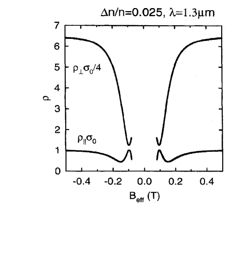
Figure 1: Plots of $\rho_{\perp}=\rho_{yy}$ and $\rho_{||}=\rho_{xx}$ in units of the Drude resistivity $\sigma_{0}^{-1}$ in zero magnetic field, as functions of the effective magnetic field $B_{eff}$ for $\Delta n/n=0.025$. Here, $n=1.1\times 10^{15}m^{-2},\ \ p_{F}=1.2\times 10^{-26}\ kg.m/s$ $\lambda=0.5\ \mu m$ and $\ell=1.0\ \mu m$.

The oscillations in both $\rho_{xx}$ and $\rho_{yy}$ are due to the density modulation and depend on the wavelength $\lambda$. The ratio $\rho_{xx}/\rho_{yy}$ for the range of magnetic fields shown in Fig. 1 is in good agreement with experiment four . In the immediate vicinity of $\nu=1/2$, where the condition $\frac{\Delta B}{B_{eff}}<1$ is not satisfied, our theory breaks down because the magnetic field dependence is strongly influenced by the channeled orbits of CFs which cannot be included in this formalism.

IV IV. Summary and Concluding Remarks

In this paper, we use a quasiclassical theory based on the Beenakker approximation for dc magnetotransport in a modulated quantum Hall system near filling factor $\nu=1/2$. Assuming that a weak one-dimensional electrostatic potential acts on the two-dimensional electron gas, we obtain closed form analytic expressions for the resistivity $\rho_{\perp}$ corresponding to a current at right angles to the direction of the modulation lines as well as a smaller component $\rho_{||}$ for a current along the direction of the modulation lines. Numerical results are presented for $\rho_{\perp}$ and $\rho_{||}$ and show some of the features observed experimentally. Our analytic results are not valid at filling factors too close to $\nu=1/2$ because our approximation scheme assumes that $\Delta B/B_{eff}$ is a small parameter which can be applied as a perturbation parameter. A completely different approach must be used for filling factors nearer $\nu=1/2$ and will be considered elsewhere.

Finally, we point out that expressions similar to our results for the magnetoresistivity in Eqs. (20) and (21) can also be used for a semiquantitative analysis of dc madnetotransport in a modulated 2DEG in a weak nonquantizing magnetic field when the modulation is magnetic in nature. This enables us to explain qualitatively the so-called “antiphase” oscillations of the magnetoresistivity $\rho_{||}.$ It was observed in experiments twelve and confirmed with the calculations based on quantum mechanical approach thirteen that both magnetoresistivity components of a 2DEG in a one-dimensional lateral superlattice show oscillations of the same period at low magnetic fields where quantum oscillations of the electron density of states at the Fermi surface (DOS) are negligible. Oscillations of $\rho_{\perp}$ are identified as a commensurability effect (Weiss oscillations) which is also described within a semiclassical approach. As for antiphase oscillations of $\rho_{||}$, the current semiclassical theory is enable to explain them, therefore it is proposed twelve ; thirteen ; fourteen ; fifteen that these oscillations are dominated by quantum mechanism, namely, by modulation-induced amplitude oscillations of DOS. The above explanation is hardly correct. It is true that at the presence of modulations quantum oscillations of DOS are superimposed with the commensurability oscillations. The same effect can be observed in conventional metals, as it was shown before eighteen . However, at low magnetic fields the quantum correction to DOS goes to zero, modulated or not. Only effects originating from classical mechanisms survive within this semiclassical limit. Besides, it is well known that periods of quantum oscillations of DOS and semiclassical commensurability oscillations differ, and their ratio is of the order of $\hbar g/p_{F}$ where $p_{F}$ is the Fermi momentum of the considered system. Based on coincidence of the periods of low field oscillations of both magnetoresistivity components we conclude that they have the same nature and origin. So, we treat the low-field oscillations of $\rho_{||}$ as semiclassical commensurability oscillations which are misinterpreted as a quantum effect by the existing theory. Our results (19) and (39) confirm this conclusion. We do not believe that this contradicts the results of thirteen based on quantum calculations. As in the case of Weiss oscillations, consistent results can be obtained within a classical approach as well as a semiclassical limit of quantum calculations, and we believe that our approach present a correct qualitative semiclassical description of the antiphase oscillations of $\rho_{||},$ restoring the self-consistence of the of the theory of magnetotransport in modulated 2D electron systems.

Acknowledgments: NAZ thanks G.M. Zimbovsky for help with the manuscript. GG acknowledges the support in part from a NATO Grant # CRG-972117 (U.S. - U.K. Collaborative Grant), the City University of New York PSC-CUNY grants #664279 and #669456 as well as grant # 4137308-02 from the NIH. JLB acknowledges support in part from an ”in service” grant from the PSC-CUNY research program.

V V. appendix

In this Appendix, we present a derivation of the expressions for the components of the magnetoresistivity based on the Boltzmann transport equation. Our goal is to show that both $\rho_{||}$ and $\rho_{\perp}$ can be affected by weak density modulations along the $y$ direction with $\Delta n(y)=\Delta n\ \sin(gy)$, where $g$ is a constant. For simplicity, we neglect a small direct effect due to the screened electric modulating potential $U(y)$ on the response functions and we concentrate on the effect of modulations of the effective magnetic field.

The CF current density can be written as

$${\bf j}(y)=Ne^{2}\int_{0}^{2\pi}\frac{d\psi}{2\pi}\ {\bf v}(\psi)\Phi(y,\psi)\ ,$$ (22)

where $N$ is the CF density of states on their Fermi surface and the distribution function $\Phi(y,\psi)$ satisfies the linearized Boltzmann equation

$$v_{y}\frac{\partial\Phi}{\partial y}+(\Omega+\Delta\Omega(y))\frac{\partial\Phi}{\partial\psi}+C[\Phi]={\bf E}\cdot{\bf v}\ .$$ (23)

Here, ${\bf E}$ is an external electric field. The collision integral $C[\Phi]$ in our calculations below is taken in a relaxation time approximation, with the relaxation towards the local equilibrium distribution function, i.e.,

$$C[\Phi]=\frac{1}{\tau}\left[\Phi(y,\psi)-\int_{0}^{2\pi}\frac{d\psi}{2\pi}\ \Phi(y,\psi)\right]\ .$$ (24)

The average of this $C[\Phi]$ over $\psi$ vanishes. As a result, the current density in Eq. (22) has to satisfy the continuity equation.

To proceed, we separate from the distribution function the homogeneous term $\Phi(\psi)$ which describes the linear response of the CF system in the absence of modulations. For this term, we use the expression given in ten , i.e.,

$$\Phi(\psi)=\rho_{0}\tau{\bf v}\cdot{\bf j}_{0}\ ,$$ (25)

where $\rho_{0}$ is the Drude resistivity ($\rho_{0}=\frac{1}{\sigma_{0}}$) and ${\bf j}_{0}$ is the CF current density for the unmodulated system.

Expressing $\Phi(y,\psi)$ as

$$\Phi(y,\psi)=\Phi(\psi)+\rho_{0}\tau\chi(y,\psi)\ ,$$ (26)

we obtain the following transport equation

$$v_{y}\frac{\partial\chi}{\partial y}+(\Omega+\Delta\Omega(y))\frac{\partial\chi}{\partial\psi}+C[\chi]=\Delta\Omega(y)\left(v_{y}j_{x}^{0}-v_{x}j_{y}^{0}\right)\ .$$ (27)

We now expand $\chi(y,\psi)$ as a Fourier series in its spatial variable, i.e.,

$$\chi(y,\psi)=\chi_{0}(\psi)+\sum_{n=1}^{\infty}\left(\chi_{n}e^{igny}+\chi_{n}^{\ast}e^{-igny}\right)\ .$$ (28)

This leads to a system of equations for the Fourier components $\chi_{n}(\psi)$ given by

$$\frac{\partial\chi_{0}}{\partial\psi} + \frac{1}{\Omega}C[\chi_{0}]=i\frac{\Delta\Omega}{2\Omega}\left(\frac{\partial\chi_{1}^{\ast}}{\partial\psi}-\frac{\partial\chi_{1}}{\partial\psi}\right),$$ (29)

$$igR\sin(\psi)\chi_{1} + \frac{\partial\chi_{1}}{\partial\psi}+\frac{1}{\Omega}C[\chi_{1}]=\frac{i}{2}\frac{\Delta\Omega}{\Omega}\left(v_{x}j_{y}^{0}-v_{y}j_{x}^{0}\right)$$ (30)

$$+ \frac{i}{2}\frac{\Delta\Omega}{\Omega}\left(\frac{\partial\chi_{0}}{\partial\psi}-\frac{\partial\chi_{2}}{\partial\psi}\right).$$

The equations determining the Fourier components $\chi_{n}$ for $n\geq 2$ are given by

$$ingR\ \chi_{n}+\frac{\partial\chi_{n}}{\partial\psi}+\frac{1}{\Omega}C[\chi_{n}]=i\frac{\Delta\Omega}{2\Omega}\left(\frac{\partial\chi_{n-1}}{\partial\psi}-\frac{\partial\chi_{n+1}}{\partial\psi}\right)\ .$$ (31)

It follows from Eqs. (29)-(31) that $\chi_{1}$ and $\chi_{1}^{\ast}$ are of the order of $\Delta B/B_{eff}$, whereas $\chi_{0},\chi_{2}$ and $\chi_{2}^{\ast}$ are of order $(\Delta B/B_{eff})^{2}$ and all Fourier components with $n>2$ are of order $(\Delta B/B_{eff})^{3}$ or smaller. Therefore, retaining in the expansion of $\chi(y,\psi)$ those terms no less than the square of $\Delta B/B_{eff}$, we can omit all terms with $n>2$ in the Fourier series (28). Then, looking for the solutions of (LABEL:ae8)-(31) in the limit when impurity scattering is weak, i.e., $\Omega\tau\gg 1$, we obtain the main approximations for the desired Fourier components, namely,

$$\chi_{0}(\psi) = \left(\frac{\Delta\Omega}{\Omega}\right)^{2}\sin(gR\cos\psi)\ QE_{x}\ ,$$ (32)

$$\chi_{1}(\psi) = \frac{\Delta\Omega}{\Omega}\exp(igR\cos\psi)\ QE_{x}\ ,$$ (33)

$$\chi_{2}(\psi) = -\frac{i}{2}\left(\frac{\Delta\Omega}{\Omega}\right)^{2}\exp(igR\cos\psi)\ QE_{x}n$$ (34)

$$+ \frac{i}{2}\left(\frac{\Delta\Omega}{\Omega}\right)^{2}\exp(2igR\cos\psi)\ SE_{x}\ ,$$

$$Q = \frac{v_{F}}{2}\sigma_{0}\Omega\tau\frac{J_{1}(gR)}{1-J_{0}^{2}(gR)}\ ,$$ (35)

$$S = \frac{v_{F}}{2}\sigma_{0}\Omega\tau\frac{J_{0}(gR)J_{1}(gR)}{(1-J_{0}^{2}(gR))(1+J_{0}(2gR))}\ .$$ (36)

Substituting the derived results in Eqs. (32)-(34) into the Fourier expansion (28), we obtain the distribution function $\chi(y,\psi)$ which we use to calculate the CF current density for a modulated system.

We see that only the $j_{x}$ component has an extra term due to the modulation, whereas $j_{y}$ remains unchanged and does not depend on the $y$ coordinate. This agrees with the continuity equation and is a motivation for us to calculate the averaged CF current density in a simple way:

$$<{\bf j}(y)>=<\tensor{\sigma}_{cf}(y)>\cdot{\bf E}\ .$$ (37)

We obtain

$$\sigma_{cf}^{xx}=<\sigma_{cf}^{xx}(y)>=\frac{\sigma_{0}}{1+(\Omega\tau)^{2}}+\sigma_{0}\left(\frac{\Delta B}{B_{eff}}\right)^{2}\frac{J_{1}^{2}(gR)}{1-J_{0}^{2}(gR)}\ .$$ (38)

The second term in (38) represents the diffusion of the CFs along the $x$ direction due to the drift of the guiding center. Other components of the CF conductivity tensor remain unchanged due to the modulation and we obtain the following expressions for the electron magnetoresistivity:

$$\rho_{yy}=\rho_{\perp}\approx\frac{1}{\sigma_{0}}\left\{1+\left(\frac{\Delta n}{n}k_{F}l\right)^{2}\frac{J_{1}^{2}(gR)}{1-J_{0}^{2}(gR)}\right\},$$ (39)

$$\rho_{xx}=\rho_{||}\approx\frac{1}{\sigma_{0}}\left\{1-\left(\frac{\Delta n}{n}k_{F}R\right)^{2}\frac{J_{1}^{2}(gR)}{1-J_{0}^{2}(gR)}\right\}.$$ (40)

These results (38), (39) are obtained using the main approximation in the expansion of the distribution function $\chi(y,\psi)$ in the expansion of the distribution function $\chi(y,\psi)$ in the inverse powers of the parameter $\Omega\tau>>1.$ Taking into account higher order terms in this expansion does not change the main result, namely, that both resistivities are influenced by the modulations. Corresponding calculations are lengthy, and we do not present them here.

So, our analysis based on the Boltzmann equation gives results which do not contradict our semiquantitative approach which we employed in Section 2. We have shown that both magnetoresistivity components are affected by the modulation, although the effect on $\rho_{\perp}$ is larger than on $\rho_{||}$. Apart from the denominator $(1-J_{0}^{2}(gR))$, the first terms in the expressions for the corrections due to modulation in our results (20) and (21) coincide with the corrections in the expressions (39) and (40).

We now return to the discrepancy between our results and those in Refs. five ; six ; seven ; eight ; nine ; ten ; eleven . We use of the definitions in ten for the effective magnetoresistivity tensor $\tensor{\rho}_{eff}\cdot<{\bf j}>={\bf E}$ and their result $\tensor{\rho}_{{\cal D}}{\bf j}={\bf E}+{\bf\Delta}$, where $\tensor{\rho}_{{\cal D}}$ is the Drude resistivity tensor and the vector ${\bf\Delta}$ is (see ten )

$$\Delta_{x,y}=\mp\frac{2\rho_{0}\tau}{v_{F}^{2}}\left<\int_{0}^{2\pi}\frac{d\psi}{2\pi}\ \Delta\Omega(y)v_{y,x}\chi(y,\psi)\right>\ .$$ (41)

We conclude that for weak modulation, when $<{\bf j}>\approx{\bf j}_{0}$, we have

$$\left(\tensor{\rho}_{{\cal D}}-\tensor{\rho}_{eff}\right)\cdot{\bf j}_{0}={\bf\Delta}\ .$$ (42)

This means that the components of the vector ${\bf\Delta}$ are linear combinations of the components of the corrections of the linear resistivity tensor. As in the local limit, the effective resistivity tensor is directly calculated in ten , avoiding calculations of the effective conductivity first.

Substituting our expression for $\chi(y,\psi)$ into (41), we can obtain ${\bf\Delta}$, and then the components of the electron magnetoresistivity. The results corroborate the corresponding results of ten and we arrive at their conclusion that only $\rho_{\perp}$ is affected by the modulation. This confirms our conclusion that the root of the disagreement between our results and those of five ; six ; seven ; eight ; nine ; ten ; eleven is in the different ways of averaging the response functions over the period of the modulation.

References

- (1) B.I. Halperin, P.A. Lee, and N.A. Read, Phys. Rev. B 47, 7312 (1993).
- (2) B.I. Halperin in “Low-Dimensional Semiconductor Structures,” edited by . Das Sarma and A. Pinczuk (Wiley, NY, 1996).
- (3) J.H S, K. von Klitzing, D. Weiss, and W. Wegschneider, Phys. Rev. Lett. 80, 4538 (1998).
- (4) R.W. Willett, K.W. West, and L.N. Pfeiffer, Phys. Rev. Lett. 83, 2624 (1999); see also the review article by R.W. Willett, Advances in Physics, 46, 447 (1997).
- (5) F. von Oppen, A. Stern, and B.I. Halperin, Phys. Rev. B 80, 4434 (1998).
- (6) A.D. Merlin, P. Wölfle, Y. Levinson, and O. Entin Wohlman, Phys. Rev. Lett. 81, 1070 (1998).
- (7) S.D.U. Zwerscke and R.R. Gerhardts, Phys. Rev. Lett. 83, 2616 (1999).
- (8) C.W.J. Beenakker, Phys. Rev. Lett. 62, 2020, (1989).
- (9) R.R. Gerhardts, Phys. Rev. B 53, 11064 (1996).
- (10) R. Menne and R.R. Gerhardts, Phys. Rev. B 57, 1707 (1998).
- (11) A.D. Mirlin and P. Wolfle, Phys. Rev. B 58, 12986 (1998).
- (12) D.Weiss, K.v. Klitzing, K. Ploog and G. Weimann, Europhys. Lett 8, 179 (1989).
- (13) C. Zhang and R.R. Gerhardts, Phys. Rev. B 41, 12850, (1990).
- (14) A. Manolescu, R.R. Gerhardts, M. Suhrke and U. Rossler, Phys. Rev. B 63, 115322 (2001).
- (15) J. Grob and R.R. Gerhardts, Phys. Rev. B 66, 155321 (2002).
- (16) Y. Levinson, O. Entin-Wohlman, A.D. Mirlin and P. Wolfle, Phys. Rev. B 58, 7113 (1998).
- (17) N.A. Zimbovskaya and J.L. Birman, Phys. Rev. B 60, 12174 (1999), Solid State Comm. 116, 21 (2000).
- (18) There is one exception, namely the paper of A.D. Mirlin and P. Wolfle eleven , where the authors claim that they first introduce the averaged effective conductivity, which seems to be the same approach as adopted in our work. However, the comparison of eleven with the work of Menne and Gerhardts ten shows that the quantity which is claimed there to be the effective conductivity actually is the different quantity, namely, an inverse of the effective magnetoresistivity tensor introduced in ten .
- (19) See e.g. N. Zimbovskaya, Local Geometry of the Fermi Surface and High-Frequency Phenomena in Metals, Ch. 7. Springer-Verlag, New York, 2001.