Hexatic$-$Herringbone Coupling at the Hexatic Transition in Smectic Liquid Crystals: $4-\epsilon$ Renormalization Group Calculations Revisited

Abstract

Simple symmetry considerations would suggest that the transition from the smectic-A phase to the long-range bond orientationally ordered hexatic smectic-B phase should belong to the XY universality class. However, a number of experimental studies have constantly reported over the past twenty years “novel” critical behavior with non-XY critical exponents for this transition. Bruinsma and Aeppli argued in Physical Review Letters 48, 1625 (1982), using a $4-\epsilon$ renormalization-group calculation, that short-range molecular herringbone correlations coupled to the hexatic ordering drive this transition first order via thermal fluctuations, and that the critical behavior observed in real systems is controlled by a ‘nearby’ tricritical point. We have revisited the model of Bruinsma and Aeppli and present here the results of our study. We have found two nontrivial strongly-coupled herringbone-hexatic fixed points apparently missed by those authors. Yet, those two new nontrivial fixed-points are unstable, and we obtain the same final conclusion as the one reached by Bruinsma and Aeppli, namely that of a fluctuation-driven first order transition. We also discuss the effect of local two-fold distortion of the bond order as a possible missing order parameter in the Hamiltonian.

]

I Introduction

The nature of phase transitions in two dimensional (2D) systems, has been the subject of numerous investigations over the last three decades. According to the Mermin-Wagner-Hohenberg theorem [2], the continuous symmetry of the XY and Heisenberg models cannot be spontaneously broken at finite temperature, and there can be no long range magnetic order. However, Kosterlitz and Thouless (KT) [3] argued that there is a new type of phase transition from a high temperature phase with exponentially decay of the correlations to a low temperature phase with power law decay of the correlations. The idea of KT has been extended by Halperin and Nelson [4] and Young [5] to the 2D melting problem. One of the main results of the KTHNY theory is the prediction of an intermediate 2D phase called the hexatic phase for systems that have a six-fold (hexagonal) symmetry in their crystalline ground state. This hexatic phase displays short range positional order, but quasi long range bond-orientational order, which is different from the true long range bond-orientational and quasi long range translational order of a 2D solid phase [4, 6]. The hexatic phase can be characterized by a bond-orientational order parameter defined by $\Psi_{6}=\mid\!\Psi_{6}\!\mid\exp(i6\psi_{6})$. Assuming that the hexatic state occurs and is not preempted by a direct first order transition from the solid to the isotropic liquid phase, the system should, in the simplest scenario for 2D, display either a KT transition or a first order transition from the hexatic state to the isotropic liquid phase [6].

It was soon realized after the proposal of the KTHNY theory that the hexatic phases, with short range positional order but true long range bond orientational order, might exist in highly anisotropic three dimensional (3D) systems. Specifically, Birgeneau and Lister [7] applied the notion of a hexatic state of the 2D melting theory to 3D liquid crystal phases consisting of stacked 2D layers. They proposed that some of the experimentally observed smectic liquid crystal phases could be physical realization of 3D hexatics. Birgeneau and Lister suggested that the (weak) interlayer interaction could promote the quasi long range order of 2D hexatic layers to true long range bond orientational order in 3D.

Stimulated by these theoretical advances, numerous experimental efforts have been undertaken to test theoretical predictions in different liquid crystal materials candidate for displaying hexatic phases [8]. An x-ray study of the liquid crystal compound 65OBC (n-alkyl-4’-m-alkoxybiphenyl-4-carboxylate,n=6,m=5) [9] provided the first indication of the existence of the 3D analog of the 2D hexatic phase. It was also found that in addition to the hexagonal pattern of diffuse spots of scattered intensity, which is the signature of the hexatic phase, there are some broader peaks corresponding to correlations in the molecular orientations about their long axes [9]. The positions of these peaks show that, locally, the molecules are packed according to a herringbone pattern perpendicular to the smectic layer stacking direction (see Fig. 1). Despite the indication of short range herringbone correlations, this novel phase is simply denoted as the hexatic-B (HexB) phase. Upon increasing temperature, this phase looses its long range bond orientational order and undergoes a transition to the smectic-A (SmA) phase, which essentially consists of a stack of 2D liquid layers. Upon cooling, the HexB phase transforms via a first order phase transition into the crystal-E (CryE) phase, which exhibits both long range translational order and long range herringbone orientational order in the orientations of the molecular axes.

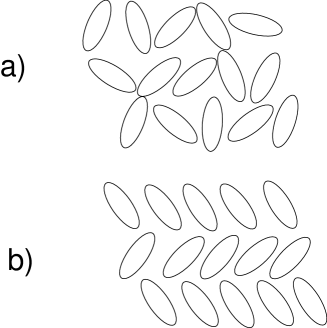
FIG. 1.: Local hexagonal coordination of the molecules ‘as seen’ along the stacking direction of the smectic layers. The elliptical shape of the molecules as seen along the stacking direction is meant to represent the “wide” benzene rings present on most thermotropic liquid crystal molecules. a) without herringbone correlations. b) with local herringbone packing correlations of the molecular axes.

According to the $U(1)$ symmetry of the $\Psi_{6}$ bond orientational order parameter, one would naively expect to find XY-like critical exponents at the SmA$-$HexB transition. However, heat capacity investigations near the SmA$-$HexB transition of 65OBC [8, 9, 10] and subsequent calorimetric studies on many other components in the nmOBC homologous series [8, 11] have constantly been reporting continuous (second order) SmA$-$HexB transitions with very large values for the heat capacity critical exponent, $\alpha\approx 0.6$. This is drastically different from the 3D XY critical exponent $\alpha=-0.007$ [12]. As well, thermal conductivity and birefringence experiments have allowed the determination of other static critical exponents, all of which differ systematically from the 3D XY value, while they, together, obey the standard scaling relationships expected for a genuine second order phase transition [8].

In the light of the existence of the short range herringbone fluctuations, detected in the x-ray diffraction studies [9], Bruinsma and Aeppli (BA) [13] formulated a Ginzburg-Landau theory that includes both the hexatic and herringbone order. Because the HexB phase exhibits only short range positional order, BA suggested that the herringbone order can also be represented by an XY order parameter described by $\Phi_{2}=\mid\!\Phi_{2}\!\mid\exp(i2\phi_{2})$. At the microscopic level, it is the molecular anisotropy that creates a coupling between the hexatic bond order and the herringbone molecular order [14, 15]. At the phenomenological Ginzburg-Landau level, this coupling is described by a hexatic-herringbone interaction term $V_{\rm hex-her}=h{\rm Re}(\Psi_{6}^{*}\Phi_{2}^{3})$.

BA constructed an appropriate free energy density based on symmetry considerations and investigated the effects of fluctuation corrections to the mean field behavior for 3D systems. In the mean field approach, their results indicate that the SmA$-$HexB transition should be continuous. However, $4-\epsilon$ renormalization group (RG) calculations, which includes thermal fluctuations and the coupling term $h{\rm Re}(\Psi_{6}^{*}\Phi_{2}^{3})$, show that short-range molecular herringbone correlations coupled to the hexatic ordering drive this transition first order, which becomes second order at a tricritical point[13].

Interestingly, heat capacity measurement studies of (truly two-dimensional) two-layer free standing films of different nmOBC compounds yield very sharp heat capacity peaks near the SmA$-$HexB transition which can be described by the critical exponent $\alpha\approx 0.3$ [8, 16].This is in sharp contrast with the usual broad and nonsingular specific heat hump associated to the KT transition in the 2D XY model, or yet the first order transition that could occur in a physical system where the vortex core energy is less than some critical value[6, 17]. This $\alpha\approx 0.3$ result further suggests that the SmA$-$HexB cannot be described by a simple model with a unique (critical) XY-like order parameter. In this context, there has been some numerical simulations done to obtain more insight into the nature of the SmA$-$HexB transition in 2D systems. The model used in the simulations [18, 19] consists of a 2D lattice of coupled XY spins based on the BA Hamiltonian. The simulation results suggest the existence of a new type phase transition in which the two different orderings are simultaneously established through a continuous transition. It is interesting to note here that, in seemingly different context, there has also been numerous theoretical and numerical attempts to identify ‘novel chiral’ universality classes for systems such as frustrated XY model and Ising-XY coupled model [20].

Certainly, for three dimensions, the scenario of a fluctuation-driven first order SmA$-$HexB transition due to hexatic$-$herringbone coupling would appear reasonable for the SmA$-$HexB transition in 65OBC which, upon further cooling, undergoes a HexB$-$CryE transition that establishes long range herringbone and positional order. However, the mixture of 3(10)OBC and PHOAB exhibits a very large temperature range for the HexB phase above the crystallization temperature to the CryE phase. If there were herringbone fluctuations near the SmA$-$HexB transition in that mixture, one could expect them to be quite small because of the large HexB temperature range, and the SmA$-$HexB transition could then possibly be continuous, and to belong to the (then naively expected) XY universality class. However, the fact that the SmA-HexB transition in the 3(10)OBC-PHOAB mixture is found to be first order does not support this simple minded argument [8]. Following the same type of reasoning, recent x-ray diffraction studies on 75OBC [8] show that the intensity of the herringbone peaks is weaker than those of 65OBC. In principle, if one assumes that 65OBC is near a tricritical point, 75OBC should therefore be further removed from this point (due to the weaker herringbone diffraction peaks, and consequently, weaker $V_{\rm hex-her}$), with again the possibility to recover 3D XY critical behavior. Yet, the same (unconventional) heat-capacity critical exponents are found for these two materials.

The experimental results above could be interpreted as a possible indication of an underlying “novel” (non-XY) stable fixed point that control the SmA$-$HexB transition when herringbone correlations are present. The apparent lack of progress on the theoretical side of the SmA$-$HexB problem has led us to reinvestigate the model of BA and to, specifically, look for a possible calculation error. Firstly, it is important to note that the conclusion of a fluctuation-driven first order within a $4-\epsilon$ calculation is acutely depending on the ‘numerics’ and not constrained by symmetry consideration: a small error (such as a factor 2 instead of 4 here or there) can change the conclusion of a fluctuation-driven first order transition. Secondly, and more specific to the BA problem, we show in the next section, when describing the Ginzburg-Landau free energy density for the SmA$-$HexB transition, that some terms in the RG equations, to first order in $\epsilon$, were missed in the work of BA. Based on our RG equations, we find two nontrivial strongly-coupled herringbone-hexatic fixed points, apparently missed by those authors. However, those two nontrivial fixed-points are unstable, and we reach the same final conclusion as the one found by BA, namely that of a fluctuation-driven first order transition. We also discuss the possibility of a third and a priori possibly physically pertinent order parameter in the Hamiltonian model of the SmA$-$HexB transition. Because of local distortion of the bond orientational order induced by the anisotropy of the intermolecular potential [14, 15] and the herringbone correlations, one may generalize the Hamiltonian to the case with three XY-like order parameters, in which two of them are two-fold symmetric, one for the herringbone correlations, $\Phi_{2}$, and one for the local two-fold distortion, $\Psi_{2}$, and a third order parameter with six-fold symmetry, $\Psi_{6}$, related to hexatic ordering. We discuss both mean field and RG calculations for this new model.

The rest of this paper is organized as follows. In Sec. II.A, we reintroduce the BA model and present the result of our RG calculations. In the Sec. II.B, we generalize the Hamiltonian to the case of three order parameter and discuss the mean field theory and RG results. The discussions and conclusions appear in Sec. III.

II Models and RG Calculations

A BA Hamiltonian

To formulate the Landau Ginzburg (LG) free energy, which describes both the hexatic and herringbone order, one recalls that the hexatic order is six-fold symmetric, while rotating a herringbone pattern by $180^{o}$ leaves it unchanged. Consequently, the appropriate LG free energy ought to be invariant with respect to the transformation $\phi_{2}(r)\rightarrow\phi_{2}(r)+n\pi$ and $\psi_{6}(r)\rightarrow\psi_{6}(r)+m(2\pi/6)$ where $n$ and $m$ are integers. Thus to lowest order in $\Psi_{6}$ and $\Phi_{2}$, the BA Hamiltonian [13] is:

$$\beta F = \int d^{3}x\;\bigg{[}\frac{r_{6}}{2}\mid\!\Psi_{6}\!\mid^{2}+\frac{1}{2}\mid\!\nabla\Psi_{6}\!\mid^{2}+\frac{r_{2}}{2}\mid\!\Phi_{2}\!\mid^{2}$$ (1)

$$+ \frac{1}{2}\mid\!\nabla\Phi_{2}\!\mid^{2}+u_{6}\mid\!\Psi_{6}\!\mid^{4}+u_{2}\mid\!\Phi_{2}\!\mid^{4}$$ (2)

$$+ w\mid\!\Phi_{2}\!\mid^{2}\mid\!\Psi_{6}\!\mid^{2}+h{\rm Re}(\Psi_{6}^{*}\Phi_{2}^{3})\bigg{]}.$$ (3)

The condition for thermodynamic stability of $F$ for $w=0$ is $h^{4/3}<(4^{4/3}/3)u_{2}u_{6}^{1/3}$. This condition can be obtained by minimizing the free energy density on the critical isothermal line $r_{2}=r_{6}=0$ and requesting that $\beta F>0$. As discussed in the Ref. [13], in the mean field approximation, for $w=0$ and $h=0$ the phase diagram in the $r_{2}-r_{6}$ plane includes four distinct phases: an isotropic (SmA) phase with $\Psi_{6}=\Phi_{2}=0$, a hexatic (HexB) phase with no herringbone order with $\Psi_{6}\neq 0,\Phi_{2}=0$, a “putative” ‘herringbone liquid crystal’ phase with $\Psi_{6}=0,\Phi_{2}\neq 0$, and a fully ordered state with $\Phi_{2}\neq 0,\Psi_{6}\neq 0$ akin to a crystalline E phase[21], with all these phases separated by second order transitions. However, if $h\neq 0$, the herringbone liquid crystal state with no hexatic order ($\Phi_{2}\neq 0,\Psi_{6}=0$) is eliminated because $\Phi_{2}$ acts as a symmetry breaking field on $\Psi_{6}$. Within mean field theory, the transition lines between the isotropic and ordered phases remain second order for $h\neq 0$, and terminate together with the first order line at a multicritical point[22].

We now discuss the RG flow equations and the stability of the fixed points (FPs). Our calculations show that the RG equations to first order in $\epsilon=4-d$ are:

$$\frac{dr_{2}}{dl}=2r_{2}+\frac{16K_{4}u_{2}}{1+r_{2}}+\frac{4K_{4}w}{1+r_{6}}$$ (4)

$$\frac{dr_{6}}{dl}=2r_{6}+\frac{16K_{4}u_{6}}{1+r_{6}}+\frac{4K_{4}w}{1+r_{2}}$$ (5)

$$\frac{du_{2}}{dl}=\epsilon u_{2}-40K_{4}u_{2}^{2}-2K_{4}w^{2}-9K_{4}h^{2}$$ (6)

$$\frac{du_{6}}{dl}=\epsilon u_{6}-40K_{4}u_{6}^{2}-2K_{4}w^{2}$$ (7)

$$\frac{dw}{dl}=\epsilon w-16K_{4}wu_{2}-16K_{4}wu_{6}-8K_{4}w^{2}-18K_{4}h^{2}$$ (8)

$$\frac{dh}{dl}=\epsilon h-24K_{4}hu_{2}-12K_{4}hw,$$ (9)

where $K_{4}=1/8\pi^{2}$. The above RG equations differ from those found by BA in Ref.[13]:

• The first set of differences are the $4K_{4}w/(1+r_{6})$ and $4K_{4}w/(1+r_{2})$ terms in the first and second equations, while BA have $2K_{4}w/(1+r_{6})$ and $2K_{4}w/(1+r_{6})$. The extra factor $2$ comes from the fact that the fields $\Psi_{6}$ and $\Phi_{2}$ are complex and the related correlations have two components. For $h=0$, Eq. (4) (with the factor $4K_{4}w$) reproduces the RG equations of coupled two components two-vector model as in previous studies[23, 24]. We therefore believe that the above RG equations for $dr_{2}/dl$ and $dr_{6}/dl$ are correct.

• Compared to the BA equations, we also obtain two completely new terms, $-18K_{4}h^{2}$, in the fifth equation and $-12K_{4}hw$ in the sixth equation, which can be easily checked using Feynmann diagram technique. Indeed, these two new terms come from the connected diagrams in the second order perturbative RG obtained by multiplication of the relevant diagrams of $h\Psi_{6}^{*}\Phi_{2}^{3}$ with $h\Psi_{6}\Phi_{2}^{*3}$, and of $w\mid\!\Phi_{2}\!\mid^{2}\mid\!\Psi_{6}\!\mid^{2}$ with $h{\rm Re}(\Psi_{6}^{*}\Phi_{2}^{3})$, respectively.

Because of the two extra terms in the RG equations for $dw/dl$ and $dh/dl$, we obtain, in addition to the simple decoupled FP ($r_{6}^{*}=r_{2}^{*}=-\epsilon/5,u_{6}^{*}=u_{2}^{*}=\epsilon/(40K_{4})$, $w^{*}=h^{*}=0$), two new fixed points such that $(w^{*}\neq 0,h^{*}=0)$ and ($w^{*}\neq 0,h^{*}\neq 0)$. The first nontrivial FP is given by $h^{*}=0,r_{6}^{*}=r_{2}^{*}=-\epsilon/4,u_{6}^{*}=u_{2}^{*}=\epsilon/(48K_{4})$, and w${}^{*}=\epsilon/(24K_{4})$. This FP, akin to the one found in minimally coupled two component two vector model [23, 24], was not discussed by BA.

However, and most interestingly, we find another “new” nontrivial mixed herringbone-hexatic FP with all the couplings being non-zero:

$$r_{6}^{*} = -0.24845566\epsilon,$$ (10)

$$r_{2}^{*} = -0.24018995\epsilon,$$ (11)

$$u_{6}^{*} = 0.01941403\epsilon/K_{4},$$ (12)

$$u_{2}^{*} = 0.01838082\epsilon/K_{4},$$ (13)

$$w^{*} = 0.04657169\epsilon/K_{4},$$ (14)

$$h^{*} = \pm 0.00766519\epsilon/K_{4}.$$ (15)

Therefore, based on our RG calculations, there is a FP with $h^{*}\neq 0$, which was not found in the previous work of BA. Linearizing the recursion relations in the vicinity of the FPs yields for the FP with ($w^{*}\neq 0$, $h^{*}=0$): $y_{1}=2-\epsilon/2,y_{2}=2-\epsilon/6,y_{3}=-\epsilon,y_{4}=-2\epsilon/3,y_{5}=y_{6}=0$. Thus, two eigenvalues are marginal, compatible with what has been found in similar minimally coupled two component two vector model [23]. The eigenvalues for the FP with ($h^{*}\neq 0,w^{*}\neq 0)$ above are

$$y_{1} = 2-0.488829\epsilon,$$ (17)

$$y_{2} = 2-0.115889\epsilon,$$ (18)

$$y_{3} = -0.997894\epsilon,$$ (19)

$$y_{4} = -0.537266\epsilon,$$ (20)

$$y_{5} = +0.121467\epsilon,$$ (21)

$$y_{6} = +0.0402392\epsilon.$$ (22)

These results show that there are four positive eigenvalues, and the above “new” nontrivial FP is therefore unstable. The two largest (most positive) eigenvalues, $y_{1}$ and $y_{2}$, correspond, respectively, to the thermal eigenvalue and the ‘relative’ coupling strength that positions the system in coupling parameter space and determines what sequence of phase transition occurs. Namely, isotropic$\rightarrow$(hexatic+herringbone) via a unique phase transtion or isotropic $\rightarrow$ hexatic $\rightarrow$(hexatic+herringbone) via two distinct phase transitions. The four eigenvalues $y_{3}$$-$$y_{6}$ essentially control the flow in the $w-h$ plane. $y_{5}$ and $y_{6}$ are positive, and we interpret the result as an indication that the above “new” nontrivial mixed herringbone-hexatic FP is unstable. Indeed, we have confirmed this by explicit numerical integration of the RG equations, and found that the RG flow goes to the unstable region identified above, which we interpret as the transition being driven first order by fluctuations. Therefore, while we have indeed found some discrepancies between our RG equations and those of BA, and recovered two extra coupled fixed points, we at the end still reach the same physical conclusion of BA, namely that of a fluctuation-driven first order smA$-$HexB transition.

B Generalized Hamiltonian

We expect physically that the local molecular anisotropy (e.g. from the anisotropic nature of benzene rings found in most thermotropic liquid crystal materials) to couple to the local bond direction, and to create a local two-fold distortion of the otherwise perfect local six-fold symmetric nearest-neighbor bond order[14, 15]. Consequently, we now discuss the LG free energy, which describes both the hexatic and herringbone order, as well as the local two-fold distortion of the bond order. If we assume that the distortion of lattice has two-fold symmetry, with the order parameter $\Psi_{2}=\mid\!\Psi_{2}\!\mid\exp(i2\psi_{2})$, then the resulting free energy is invariant under the transformation $\phi_{2}(r)\rightarrow\phi_{2}(r)+n\pi$, $\psi_{6}(r)\rightarrow\psi_{6}(r)+m(2\pi/6)$, and $\psi_{2}(r)\rightarrow\psi_{2}(r)+p\pi$ where $n$, $m$, and $p$ are integers.

From an RG point of view, our motivation to expand the symmetry of our Hamiltonian stems from the observation that in $N$ coupled 2-vector models a new stable fixed points (called mixed fixed point [23, 24]) appears in the coupling parameter space (when $N>2$). Thus, to lowest order in $\Psi_{6}$, $\Phi_{2}$, and $\Psi_{2}$, we have $\beta F=\beta F_{0}+U$, where the Gaussian part is given by

$$\beta F_{0} = \frac{1}{2}\int d^{3}x\;\bigg{[}r_{6}\mid\!\Psi_{6}\!\mid^{2}+r_{2}\mid\!\Phi_{2}\!\mid^{2}+\tilde{r}_{2}\mid\!\Psi_{2}\!\mid^{2}$$ (23)

$$+ 2r{\rm Re}(\Phi_{2}\Psi_{2}^{*})+\mid\!\nabla\Psi_{6}\!\mid^{2}+\mid\!\nabla\Phi_{2}\!\mid^{2}$$ (24)

$$+ \mid\!\nabla\Psi_{2}\!\mid^{2}+2g{\rm Re}(\nabla\Phi_{2}\nabla\Psi_{2}^{*})\bigg{]},$$ (25)

and the perturbative Hamiltonian has the following form[25]:

$$U = \int d^{3}x\;\bigg{[}u_{6}\mid\!\Psi_{6}\!\mid^{4}+u_{2}\mid\!\Phi_{2}\!\mid^{4}+\tilde{u}_{2}\mid\!\Psi_{2}\!\mid^{4}$$ (26)

$$+ w_{1}\mid\!\Psi_{6}\!\mid^{2}\mid\!\Phi_{2}\!\mid^{2}+w_{2}\mid\!\Psi_{6}\!\mid^{2}\mid\!\Psi_{2}\!\mid^{2}+w_{3}\mid\!\Phi_{2}\!\mid^{2}\mid\!\Psi_{2}\!\mid^{2}$$ (27)

$$+ h_{1}{\rm Re}(\Psi_{6}^{*}\Phi_{2}^{3})+h_{2}{\rm Re}(\Psi_{6}^{*}\Psi_{2}^{3})+h_{3}{\rm Re}(\Phi_{2}^{2}\Psi_{2}^{*2})$$ (28)

$$+ v_{1}{\rm Re}(\Psi_{6}^{*}\Phi_{2}\Psi_{2}^{2})+v_{2}{\rm Re}(\Psi_{6}^{*}\Phi_{2}^{2}\Psi_{2})+v_{3}\mid\!\Psi_{6}\!\mid^{2}{\rm Re}(\Phi_{2}\Psi_{2}^{*})$$ (29)

$$+ v_{4}\mid\!\Phi_{2}\!\mid^{2}{\rm Re}(\Phi_{2}\Psi_{2}^{*})+v_{5}\mid\!\Psi_{2}\!\mid^{2}{\rm Re}(\Phi_{2}\Psi_{2}^{*})\bigg{]}$$ (30)

For the case that $r_{2}=\tilde{r}_{2}$, one can simply diagonalize the Gaussian part of the Hamiltonian using the transformation $\Phi_{2}=(\tilde{\Phi}_{2}+\tilde{\Psi}_{2})/\sqrt{2}$ and $\Psi_{2}=(\tilde{\Phi}_{2}-\tilde{\Psi}_{2})/\sqrt{2}$, and then do the RG calculations. The RG calculations for the case that $\Psi_{6}=0$ were done by Yosefin and Domany [26] in the study of the phase transitions in fully frustrated XY models

In the mean field approach, there are now four distinct phases for $r\neq 0$ ($\Psi_{6}=\Phi_{2}=\Psi_{2}=0;\Psi_{6}=0,\Phi_{2}\neq 0,\Psi_{2}\neq 0;\Psi_{6}\neq 0,\Psi_{2}=\Phi_{2}=0;\Psi_{6}\neq 0,\Psi_{2}\neq 0,\Phi_{2}\neq 0$). One should note that for the phases where both $\Phi_{2}$ and $\Psi_{2}$ are non-zero, we have the condition of local stability of the free energy, $r_{2}\tilde{r}_{2}<r^{2}$. In addition, the singularity of the propagators at zero wavevector (${\bf q})=0$) is for $r_{2}\tilde{r}_{2}=r^{2}$, which is the critical point of the system.

To obtain further insight into the specific situation where both $\Phi_{2}$ and $\Psi_{2}$ go simultaneously critical (soft), we perform an RG calculation. To simplify the calculations, we consider the case that $r_{2}=\tilde{r}_{2}$, so that the fields $\Phi_{2}$ and $\Psi_{2}$ are simultaneously critical (soft), and that they are equally coupled to the $\Psi_{6}$ hexatic field ($u_{2}=\tilde{u}_{2}$, $w_{1}=w_{2}$). We further need to require that the full theory, after diagonalization of the gaussian part, is self-consistent with no new RG-generated terms. This imposes that $h_{1}=h_{2}$ and $v_{1}=v_{2}$. Using the above mentioned transformation for $\Phi_{2}$ and $\Psi_{2}$ and rescaling the fields, one can rewrite the Hamiltonian as,

$$\beta F=\int d^{3}x\;\bigg{[}\frac{r_{6}}{2}\mid\!\Psi_{6}\!\mid^{2}+\frac{r_{2}^{\prime}}{2}\mid\!\tilde{\Phi}_{2}\!\mid^{2}+\frac{\tilde{r}_{2}^{\prime}}{2}\mid\!\tilde{\Psi}_{2}\!\mid^{2}$$ (31)

$$+\frac{1}{2}\mid\!\nabla\Phi_{6}\!\mid^{2}+\frac{1}{2}\mid\!\nabla\tilde{\Phi}_{2}\!\mid^{2}+\frac{1}{2}\mid\!\nabla\tilde{\Psi}_{2}\!\mid^{2}+u_{6}\mid\!\Psi_{6}\!\mid^{4}$$ (32)

$$+u_{2}^{\prime}\mid\!\tilde{\Phi}_{2}\!\mid^{4}+\tilde{u}_{2}^{\prime}\mid\!\tilde{\Psi}_{2}\!\mid^{4}+w_{1}^{\prime}\mid\!\Psi_{6}\!\mid^{2}\mid\!\tilde{\Phi}_{2}\!\mid^{2}$$ (33)

$$+w^{\prime}_{2}\mid\!\Psi_{6}\!\mid^{2}\mid\!\tilde{\Psi}_{2}\!\mid^{2}+w_{3}^{\prime}\mid\!\tilde{\Phi}_{2}\!\mid^{2}\mid\!\tilde{\Psi}_{2}\!\mid^{2}$$ (34)

$$+h_{1}^{\prime}{\rm Re}(\Psi_{6}^{*}\tilde{\Phi}_{2}^{3})+h_{3}^{\prime}{\rm Re}(\tilde{\Phi}_{2}^{2}\tilde{\Psi}_{2}^{*2})+v_{1}^{\prime}{\rm Re}(\Psi_{6}^{*}\tilde{\Phi}_{2}\tilde{\Psi}_{2}^{2})\bigg{]},$$ (35)

where the new (primed) coefficients can be written in terms of old coefficients. To first order of $\epsilon$, the RG equations are given by,

$$\frac{dr_{6}}{dl} = 2r_{6}+\frac{16K_{4}u_{6}}{1+r_{6}}+\frac{4K_{4}w_{1}^{\prime}}{1+r_{2}^{\prime}}+\frac{4K_{4}w_{2}^{\prime}}{1+\tilde{r}_{2}^{\prime}}$$ (36)

$$\frac{dr_{2}^{\prime}}{dl} = 2r_{2}^{\prime}+\frac{16K_{4}u_{2}^{\prime}}{1+r_{2}^{\prime}}+\frac{4K_{4}w_{1}^{\prime}}{1+r_{6}}+\frac{4K_{4}w_{3}^{\prime}}{1+\tilde{r}_{2}^{\prime}}$$ (37)

$$\frac{d\tilde{r}_{2}^{\prime}}{dl} = 2\tilde{r}_{2}^{\prime}+\frac{16K_{4}\tilde{u}_{2}^{\prime}}{1+\tilde{r}_{2}^{\prime}}+\frac{4K_{4}w_{2}^{\prime}}{1+r_{6}}+\frac{4K_{4}w_{3}^{\prime}}{1+r_{2}^{\prime}}$$ (38)

$$\frac{du_{6}}{dl} = \epsilon u_{6}-40K_{4}u_{6}^{2}-2K_{4}w_{1}^{\prime 2}-2K_{4}w_{2}^{\prime 2}$$ (39)

$$\frac{du_{2}^{\prime}}{dl} = \epsilon u_{2}^{\prime}-40K_{4}u_{2}^{\prime 2}-2K_{4}w_{1}^{\prime 2}-2K_{4}w_{3}^{\prime 2}-9K_{4}h_{1}^{\prime 2}$$ (40)

$$- 2K_{4}h_{3}^{\prime 2}$$ (41)

$$\frac{d\tilde{u}_{2}^{\prime}}{dl} = \epsilon\tilde{u}_{2}^{\prime}-40K_{4}\tilde{u}_{2}^{\prime 2}-2K_{4}w_{2}^{\prime 2}-2K_{4}w_{3}^{\prime 2}-2K_{4}h_{3}^{\prime 2}$$ (42)

$$- K_{4}v_{1}^{\prime 2}$$ (43)

$$\frac{dw_{1}^{\prime}}{dl} = \epsilon w_{1}^{\prime}-16K_{4}u_{6}w_{1}^{\prime}-16K_{4}u_{2}^{\prime}w_{1}^{\prime}-8K_{4}w_{1}^{\prime 2}$$ (44)

$$- 4K_{4}w_{2}^{\prime}w_{3}^{\prime}-18K_{4}h_{1}^{\prime 2}-2K_{4}v_{1}^{\prime 2}$$ (45)

$$\frac{dw_{2}^{\prime}}{dl} = \epsilon w_{2}^{\prime}-16K_{4}u_{6}w_{2}^{\prime}-16K_{4}\tilde{u}_{2}^{\prime}w_{2}^{\prime}-8K_{4}w_{2}^{\prime 2}$$ (46)

$$- 4K_{4}w_{1}^{\prime}w_{3}^{\prime}-4K_{4}v_{1}^{\prime 2}$$ (47)

$$\frac{dw_{3}^{\prime}}{dl} = \epsilon w_{3}^{\prime}-16K_{4}u_{2}^{\prime}w_{3}^{\prime}-16K_{4}\tilde{u}_{2}^{\prime}w_{3}^{\prime}-8K_{4}w_{3}^{\prime 2}$$ (48)

$$- 4K_{4}w_{1}^{\prime}w_{2}^{\prime}-16K_{4}(h_{3}^{\prime})^{2}-4K_{4}v_{1}^{\prime 2}$$ (49)

$$\frac{dh_{1}^{\prime}}{dl} = \epsilon h_{1}^{\prime}-24K_{4}h_{1}^{\prime}u_{2}^{\prime}-12K_{4}w_{1}^{\prime}h_{1}^{\prime}-4K_{4}v_{1}^{\prime}h_{3}^{\prime}$$ (50)

$$\frac{dh_{3}^{\prime}}{dl} = \epsilon h_{3}^{\prime}-8K_{4}u_{2}^{\prime}h_{3}^{\prime}-8K_{4}\tilde{u}_{2}^{\prime}h_{3}^{\prime}-16K_{4}w_{3}^{\prime}h_{3}^{\prime}$$ (51)

$$- 6K_{4}h_{1}^{\prime}v_{1}^{\prime}$$ (52)

$$\frac{dv_{1}^{\prime}}{dl} = \epsilon v_{1}^{\prime}-8K_{4}v_{1}^{\prime}\tilde{u}_{2}^{\prime}-4K_{4}w_{1}^{\prime}v_{1}^{\prime}-8K_{4}w_{2}^{\prime}v_{1}^{\prime}$$ (53)

$$- 8K_{4}w_{3}^{\prime}v_{1}^{\prime}-12K_{4}h_{1}^{\prime}h_{3}^{\prime}.$$ (54)

We have found a number of FPs for the above RG equations that fulfill the condition ($r_{2}^{*}=\tilde{r}_{2}^{*}$, and for which $u_{2}^{*}=\tilde{u}_{2}^{*}$, $w_{1}^{*}=w_{2}^{*}$, $h_{1}^{*}=h_{2}^{*}$, $v_{1}^{*}=v_{2}^{*}$ and $v_{4}^{*}=v_{5}^{*}$). Some of these are given in the Table I, where each column correspond to a different FP (the nontrivial mixed herringbone-hexatic FP found in Section IIa occurs here as well, but is again unstable). As in the simplest case of Hamiltonian (2.1), none of the FP correspond to a nontrivial stable fixed point: each fixed point (column) shows more than two positive eigenvalues. Given the complexity of those nonlinear equations we cannot be 100% sure that we have found all the (unstable) FP in the $(u_{6},u_{6}^{\prime},\tilde{u}_{2}^{\prime},w_{1}^{\prime},w_{3}^{\prime},h_{1}^{\prime},h_{3}^{\prime},v_{1}^{\prime})$ plane. However, a numerical investigation of the RG flow in that plane starting from a large number of initial values for the coupling parameters always failed to converge towards a stable (attractive) fixed point. Therefore, we reach the same conclusion obtained in the previous section, namely that of a fluctuation-driven first order transition for this expanded symmetry Hamiltonian, and the stabilization of novel fixed point in $N$ coupled two vector models for $N>2$ does not appear to occur in this generalized Hamiltonian due to the extra coupling parameters.

Table I: The FPs of RG equations for generalized Hamiltonian.

$r_{6}^{\prime*}/\epsilon$	-1/5	-3/11	-2/7	0	-0.2761944898	-0.2583527792	-0.2727272730
$r_{2}^{\prime*}/\epsilon$	-1/5	-3/11	-2/7	-1/5	-0.2761944898	-0.2756996328	-0.2727272730
$\tilde{r}_{2}^{\prime*}/\epsilon$	-1/5	-3/11	-2/7	-1/5	-0.2566490108	-0.2756996328	-0.2727272724
$u_{6}^{\prime*}(K_{4}/\epsilon)$	1/40	1/44	1/56	0	0.0202792491	0.0237809941	0.0227272727
$u_{2}^{\prime*}(K_{4}/\epsilon)$	1/40	1/44	1/56	0.0125	0.0202792491	0.0194412033	0.0170454546
$\tilde{u}_{2}^{\prime*}(K_{4}/\epsilon)$	1/40	1/44	1/56	0.0125	0.0238702512	0.0194412033	0.0170454546
$w_{1}^{\prime*}(K_{4}/\epsilon)$	0	1/44	1/28	0	0.0405584982	0.0170262066	0.0227272727
$w_{2}^{\prime*}(K_{4}/\epsilon)$	0	1/44	1/28	0	0.0164217503	0.0170262066	0.0227272727
$w_{3}^{\prime*}(K_{4}/\epsilon)$	0	1/44	1/28	0.05	0.0164217503	0.0430587966	0.0454545454
$h_{1}^{\prime*}(K_{4}/\epsilon)$	0	1/44	0	0	0	0	0
$h_{3}^{\prime*}(K_{4}/\epsilon)$	0	1/44	0	$\pm$ 0.025	0	$\pm$ 0.0041763898	$\pm$ 0.0113636364
$v_{1}^{\prime*}(K_{4}/\epsilon)$	0	1/44	0	0	0	0	0

III Discussion

In Section II. A, we found that there are two “new” FPs missed in Ref. [13]. However, those FPs are unstable, and we reach the same final conclusion as Bruinsma and Aeppli, namely that the SmA$-$HexB transition is driven first order by fluctuations in the BA Hamiltonian. We also discussed a slightly modified simple model that considers not only the hexatic and herringbone order, but also one that involves the local two-fold deformation of the bond correlations induced by the herringbone correlations. We assumed that this deformation can be represented by a two-fold symmetry order parameter, as in the case of herringbone order, and wrote the free energy based on symmetry arguments. We were not able to find a new stable FP which could possibly result in unconventional (“new”) second order critical exponents.

It is not clear to us in what directions to pursue the paradoxical puzzle of “new universality” (non $3D$ XY transition) in hexatic liquid crystal materials. In the work presented here, we have found a novel “mixed” hexatic-herringbone fixed point in the theory, but which is unstable to first order in $\epsilon$. One note that the two positives eigenvalues $y_{5}$ and $y_{6}$ in Eq. 2.4 are only very slightly positive for $\epsilon=1$. This observation may open the possibility that in a calculation that includes hexatic-herringbone coupling, there is no stable fixed point to lowest order in $\epsilon$, but that the fixed point may be stabilized in a theory that goes beyond an $O(\epsilon^{1})$ calculation. This is what happens, for example, in the normal to superconducting phase transition where the $\epsilon$ expansion to order $\epsilon^{1}$ predicts a fluctuation-driven first order phase transition[27] while theoretical arguments and Monte Carlo simulations strongly argue for a second order (inverted 3D XY) phase transition[28].

.

Having said that, one should note that there are experiments on liquid crystal materials that do not display any herringbone correlations  [29, 30] but still show a SmA$-$HexB transition with exponents that differ from the critical behavior expected to a $2D$ [29] or $3D$[30] XY critical behavior. That may suggest that the whole idea of hexatic$-$herringbone interactions is a red herring. Another possibility is that of (more subtle) ‘hidden’ order parameter(s) distinct from the herringbone order characterizes the SmA$-$HexB transition in real materials, and that the coupling between this hidden order parameter and the hexatic order parameter $\Psi_{6}$ produces a novel stable fixed point. Clearly, more experimental studies are needed to shed light on this problem. In particular, high resolution scattering experiments would seem necessary to search for extended short-range correlation in either molecular correlations or distortion of hexagonal co-ordination to shed some light on what such ‘hidden’ order parameter(s) may be.

We finally note that a related (unconventional critical behavior) situation arises in the context of layered systems of smectic liquid crystals studied by Defontaines and Prost [31]. These authors have argued that critical points that do not involve any symmetry change can define a set of new universality classes in layered systems. Possibly, considerations of some features of the Defontaines and Prost theory may be useful in further investigations of the SmA$-$HexB problem.

We hope that our work and reinvestigation of the long standing SmA$-$Hex-B transition in smectic liquid crystal materials will motivate further theoretical, numerical and experimental investigations of this very interesting problem.

IV Acknowledgements

We thank Ian Affleck, Igor Herbut and and Mehran Kardar for useful discussions. M. G. thanks C. C. Huang for stimulating his interest in the problem of the critical behavior of the SmA$-$HexB transition. This research has been funded by NSERC of Canada. M. G. acknowledges the Research Corporation and the Province of Ontario for generous financial support.

REFERENCES

- [1]
- [2] N. D. Mermin and H. Wagner, Phys. Rev. Lett. 22, 1133 (1966); Hohenberg, Phys. Rev. 158, 383 (1967).
- [3] J. M. Kosterlitz and D. J. Thouless, J. Phys. C 6, 1181 (1973); J. M. Kosterlitz, J. Phys. C 7, 1046 (1974).
- [4] B. I. Halperin and D. R. Nelson, Phys. Rev. Lett. 41, 121 (1978); D. R. Nelson and B. I. Halperin, Phys. Rev. B 19, 2457 (1979).
- [5] A. P. Young, Phys. Rev. B 19, 1855 (1979).
- [6] K. J. Strandburg, Rev. Mod. Phys. 60, 161 (1988).
- [7] R. J. Birgeneau and J. D. Lister, J. Phys., Paris, Lett. 39, L339 (1978).
- [8] C. C. Huang and T. Stoebe, Advances in Physics 42, 343 (1993); T. Stoebe and C. C. Huang, Int. J. Mod. Phys. B 9, 2285 (1995).
- [9] R. Pindak et al., Phys. Rev. Lett. 46, 1135 (1981).
- [10] C. C. Huang, et al., Phys. Rev. Lett. 46, 1289 (1981).
- [11] T. Pitchford et al., Phys. Rev. A 32, 1938 (1985).
- [12] J. C. Le Guillou and J. Zinn Justin, J. Phys., Paris, Lett. 46, L137 (1985).
- [13] R. Bruinsma and G. Aeppli, Phys. Rev. Lett 48, 1626 (1982).
- [14] A transition in a two dimensional model of an anisotropic liquid crystal with induced bond order is discussed in: M.J.P. Gingras, P.C.W. Holdsworth and B. Bergersen, Europhys. Lett. 9, 539 (1989); ibid, Phys. Rev. A 41, 3377 (1990); ibid, Phys. Rev. A 41, 6786 (1990).
- [15] The effect of the anisotropy of the intermolecular potential on the locking between molecular order and bond order is examined in: M.J.P. Gingras, P.C.W. Holdsworth and B. Bergersen, Mol. Cryst. Liq. Cryst. 204, 177 (1991).
- [16] T. Stoebe, C. C. Huang, and J. W. Goodby, Phys. Rev. Lett. 68, 2944 (1992).
- [17] P. Minnhagen, Rev. Mod. Phys. 59, 1001 (1987).
- [18] I. M. Jiang et al., Phys. Rev. E 48, R3240 (1993).
- [19] I. M. Jiang, T. Stoebe and C. C. Huang, Phys. Rev. Lett. 76, 2910 (1996).
- [20] J. Lee et al. Phys. Rev. B 44, 4819 (1991); E. Granato et al., Phys. Rev. Lett. 66, 1090 (1991).
- [21] The parametrization of the crystalline E phase should also include a third order parameter: the amplitude of the Fourier transform of the mass density at the Bragg reciprocical wave vector.
- [22] The liquid crystal phase discussed here is, at least at the Ginzburg-Landau level considered, equivalent to the 2D locked hexatic-nematic state as mentioned by Nelson and Halperin in Phys. Rev. B 21, 5312 (1980), and investigated via Monte Carlo simulations in Ref. [15].
- [23] A. Aharony, Phase transitions and Critical Phenomena, Vol. 6, edited by C. Domb and M. S. Green, Academic Press (1976).
- [24] E. Brezin, J. C. Le Guillou, and J. Zinn-Justin, Phys. Rev. B 10, 892 (1974).
- [25] It is worth noting that we implicitely make the assumption here that the effective symmetry-breaking fields that couple the , and fields are assumed to have an homogeneous and constant phase relationship arbitrarily set to zero in spirit to the theories used in Refs. [13, 22]. In other words, the Ginzburg-Landau-Wilson free energies for the smetic-Ahexatic-B problem are not local gauge theories.
- [26] M. Yosefin and E. Domany, Phys. Rev. B 32, 178 (1985).
- [27] B.I. Halperin, T.C. Lubensky and S.K.Ma, Phys. Rev. Lett. 32, 292 (1974).
- [28] C. Dasgupta and B.I. Halperin, Phys. Rev. Lett. 47, 1556 (1981).
- [29] A.J. Jin et al. Phys. Rev. Lett. 74, 4863 (1995); ibid, Phys. Rev. E 53, 3639 (1996).
- [30] E. Górecka et al., Phys. Rev. E 50, 2863 (1994).
- [31] A. D. Defontaines and J. Prost, Phys. Rev. E 47, 1184 (1993).