Variational perturbation approach to the Coulomb electron gas

Abstract

The efficiency of the variational perturbation theory [Phys. Rev. C 62, 045503 (2000)] formulated recently for many-particle systems is examined by calculating the ground state correlation energy of the 3D electron gas with the Coulomb interaction. The perturbation beyond a variational result can be carried out systematically by the modified Wick’s theorem which defines a contraction rule about the renormalized perturbation. Utilizing the theorem, variational ring diagrams of the electron gas are summed up. As a result, the correlation energy is found to be much closer to the result of the Green’s function Monte Carlo calculation than that of the conventional ring approximation is.

I Introduction

A variational method has been widely used as a convenient and powerful tool to calculate physical quantities such as energy and order parameters [1-5]. The most important advantage of this approach consists in its applicability even for the strongly correlated systems through suitable trial wavefunctions. However, it is extremely difficult to improve the results for the systems with many degrees of freedom. In contrast, results of the perturbative approach are systematically improved by calculating the further corrections using the Feynmann rule [6-8]. However, the convergency can not be guaranteed in the unweakly coupled cases.

There have appeared many efforts trying to combine the above two approaches in order to overcome each drawback [9-14]. Many studies have been performed mainly in the areas of relativistic field theories and quantum mechanics under the principle of minimal sensitivity (PMS) [9], which says that approximated physical quantities in the perturbation theory should be minimized with respect to the parameters absent in the original Hamiltonian. These studies are called optimized perturbation theory or variational perturbation theory (VPT), which is applied very successfully to quantum mechanical problems such as the anharmonic oscillator and the double-well potential. However, we are faced with extremely complex higher-order calculations in the case of quantum field theories.

Recently, papers on another kind of VPT have been published [15-18]. This approach is not related to the PMS, because the minimization is carried out at the zeroth order and the variational parameters are fixed before the perturbative calculation. It has a simple expansion rule, which makes the VPT approach to many-particle systems more manageable. In this paper, the VPT for fermion systems of ref. [17] is briefly reviewed, and as a test on the efficiency of the method, we calculate the ground state correlation energy of the three dimensional Coulomb electron gas within a ring approximation.

II Variational perturbation theory

In this section, we briefly review the VPT in the functional integral formalism [17]. The partition function for fermion systems with two-body interaction is generally given by

$$Z=\int D[\bar{\psi}\psi]\ \exp({-G_{ij}^{o^{-1}}\bar{\psi}_{i}\psi_{j}-V_{ijkl}\bar{\psi}_{i}\bar{\psi}_{j}\psi_{k}\psi_{l}})\ ,$$ (1)

where $\bar{\psi}_{i}$,$\psi_{i}$ are Grassmann variables and each subscript stands for all possible quantum numbers including an imaginary time. The integration and summation symbols are omitted by the summation convention. Here, $G^{o}$ is the bare Green’s function matrix and $V$ is an interaction tensor. The second term of the exponent in Eq.(1) is the perturbative term in the conventional perturbation theory. Now, introducing a variational Green’s function $G$, the exponent is rewritten as

$$-G_{ij}^{-1}\bar{\psi}_{i}\psi_{j}-(G_{ij}^{o^{-1}}-G_{ij}^{-1})\bar{\psi}_{i}\psi_{j}-V_{ijkl}\bar{\psi}_{i}\bar{\psi}_{j}\psi_{k}\psi_{l}\ .$$ (2)

Then, the second and third terms in Eq.(2) are regarded as a renormalized interaction. According to the Jensen-Peierls’ inequality [19,20], we get the inequality between the thermodynamic potential $\Omega$ and the variational thermodynamic potential $\bar{\Omega}(G)$; $\Omega\leq\bar{\Omega}(G)$. Minimizing $\bar{\Omega}(G)$ with respect to $G$, we obtain an equation of $G$ as

$$G^{-1}-G^{o^{-1}}+\Sigma=0\ ,$$ (3)

where $\left<b|\Sigma|a\right>\equiv 2(V_{ibaj}-V_{biaj})G_{ji}$. We note that $G$ corresponds to the self-consistent Hartree-Fock Green’s function for the interacting fermion system. Using the condition Eq.(3), the minimized variational thermodynamic potential $\bar{\Omega}_{\rm min}$ and the correction part $\Delta\Omega\equiv\Omega-\bar{\Omega}_{\rm min}$ are arranged as follows, according to the notation in ref.[17];

$$\bar{\Omega}_{\rm min}=\frac{1}{\beta}{\rm Tr}\ln G-\frac{1}{2\beta}{\rm Tr}\Sigma G\ ,$$ (4)

$$\Delta\Omega=-\frac{1}{\beta}\left<\exp\left[-V_{ijkl}\left(\partial_{\eta_{i}}\partial_{\eta_{j}}\partial_{\bar{\eta}_{k}}\partial_{\bar{\eta}_{l}}\right)^{\prime}\right]\right>_{G,C}\ ,$$ (5)

where $\left<\cdot\cdot\cdot\right>_{G}\equiv\cdot\cdot\cdot e^{\bar{\eta}_{i}G_{ij}\eta_{j}}|_{\bar{\eta},\eta=0}$ represents the thermal average using $G$ and the subscript $C$ indicates the connected contractions among all possible contractions by the modified Wick’s theorem Eq.(7) below. During the derivation of the above equations, Grassmann variables $\bar{\eta}$, $\eta$ are introduced as source fields of the original fields $\psi$, $\bar{\psi}$, and the renormalized interaction of Eq.(2) is expressed as functional derivatives about source fields. After integrating out the Gaussian integral ($\int D[\bar{\psi}\psi]\exp(-\bar{\psi}_{i}G_{ij}^{-1}\psi_{j}+\bar{\eta}_{i}\psi_{i}+\bar{\psi}_{i}\eta_{i})={\rm Det}G^{-1}e^{\bar{\eta}_{i}G_{ij}\eta_{j}}$) and rearranging the thermodynamic potential under the condition Eq.(3), we obtain Eqs.(4) and (5). Here, the primed derivative operation $(\cdot\cdot\cdot)^{\prime}$ is defined as

$$\left(\partial_{\eta_{i}}\partial_{\eta_{j}}\partial_{\bar{\eta}_{k}}\partial_{\bar{\eta}_{l}}\right)^{\prime}$$

$$\equiv\left(\partial_{\eta_{i}}\partial_{\eta_{j}}\partial_{\bar{\eta}_{k}}\partial_{\bar{\eta}_{l}}-G_{li}\partial_{\eta_{j}}\partial_{\bar{\eta}_{k}}-G_{kj}\partial_{\eta_{i}}\partial_{\bar{\eta}_{l}}\right.$$

$$\ \ \ +\left.G_{lj}\partial_{\eta_{i}}\partial_{\bar{\eta}_{k}}+G_{ki}\partial_{\eta_{j}}\partial_{\bar{\eta}_{l}}+G_{li}G_{kj}-G_{lj}G_{ki}\right)\ .$$ (6)

Carrying out the nth order calculation of the above operation, we find modified Wick’s theorem for the perturbative expansion of the present VPT as

$$\left<\left(\partial_{\eta_{i_{1}}}\partial_{\eta_{j_{1}}}\partial_{\bar{\eta}_{k_{1}}}\partial_{\bar{\eta}_{l_{1}}}\right)^{\prime}\cdot\cdot\cdot\left(\partial_{\eta_{i_{n}}}\partial_{\eta_{j_{n}}}\partial_{\bar{\eta}_{k_{n}}}\partial_{\bar{\eta}_{l_{n}}}\right)^{\prime}\right>_{G}$$

$$={\rm Sum\ of\ all\ possible\ contractions}$$

$$\ \ {\rm\ between\ different\ cells}.$$ (7)

Here we call one $(\cdot\cdot\cdot)^{\prime}$ a unit cell and the contraction rule is as follows; each $\partial_{\eta_{i}}$ is paired with a $\partial_{\bar{\eta}_{j}}$ in a different cell and then, each pair of derivatives $\partial_{\eta_{i}}\partial_{\bar{\eta}_{j}}$ is replaced by Green’s function $G_{ji}$. In this pairing, every permutation of two derivatives changes the sign. The differences from the original Wick’s theorem are to forbid the intracell contraction and to use the renormalized Green’s function $G$. The unit cell with an interaction, $V_{ijkl}\left(\partial_{\eta_{i}}\partial_{\eta_{j}}\partial_{\bar{\eta}_{k}}\partial_{\bar{\eta}_{l}}\right)^{\prime}$, can be described by a diagram as in Fig.1 (a). A contraction is to join two incomming and outgoing lines together and to assign it a propagator $G$ which corresponds to a double line. In Fig.1 (b), we show ring diagrams with renormalized propagators, where the first order diagram does not exist because it is an intracell-joining diagram.

For example, the second order perturbation of $\Delta\Omega$ is given by;

$$-\frac{1}{\beta}V_{ijkl}V_{i^{\prime}j^{\prime}k^{\prime}l^{\prime}}G_{l^{\prime}i}G_{k^{\prime}j}G_{kj^{\prime}}G_{li^{\prime}}$$

$$+\frac{1}{\beta}V_{ijkl}V_{i^{\prime}j^{\prime}k^{\prime}l^{\prime}}G_{l^{\prime}i}G_{k^{\prime}j}G_{ki^{\prime}}G_{lj^{\prime}}\ .$$ (8)

Figure 1: (a) Unit cell to construct Feynmann diagrams; (b) the summation of variational ring diagrams. the first order diagram cannot exist in the present theory.

III Coulomb Electron Gas

The present formulation can be easily applied to any fermion systems with two-body interaction. In this section, the ground state correlation energy of the three dimensional Coulomb electron gas is calculated using the variational ring approximation which is described by ring diagrams in Fig.1 (b). The model Hamiltonian is given by

$$H=\sum_{k\sigma}\epsilon_{k}a_{k\sigma}^{\dagger}a_{k\sigma}+\frac{1}{2}\sum_{kk^{\prime}q\sigma\sigma^{\prime}}^{{}^{\prime}}v(q)a_{k\sigma}^{\dagger}a_{k^{\prime}\sigma^{\prime}}^{\dagger}a_{k^{\prime}-q\sigma^{\prime}}a_{k+q\sigma}\ ,$$ (9)

where $a_{k\sigma}^{\dagger}$($a_{k\sigma}$) is a creation(annihilation) operator of an electron with wavevector $k$ and spin $\sigma$. We have defined $\epsilon_{k}=\hbar^{2}k^{2}/2m_{e}$ and $v(q)=4\pi e^{2}/Vq^{2}$. Here, $V$, $m_{e}$ and $e$ are the system volume, the electron mass and charge respectively. The primed summation indicates that the $q=0$ term is excluded because of the cancellation with the positively charged background. In this model, the interaction $V_{ijkl}$ of Eq.(1) is expressed as

$$V_{ijkl} \rightarrow V_{k_{1}\sigma_{1}\tau_{1},k_{2}\sigma_{2}\tau_{2},k_{3}\sigma_{3}\tau_{3},k_{4}\sigma_{4}\tau_{4}}$$ (10)

$$= \frac{1}{2}v(|k_{4}-k_{1}|)\delta_{k_{1}+k_{2},k_{3}+k_{4}}\delta_{\sigma_{1}\sigma_{4}}\delta_{\sigma_{2}\sigma_{3}}$$

$$\times \delta(\tau_{1}-\tau_{2})\delta(\tau_{3}-\tau_{4})\delta(\tau_{2}-\tau_{3})\ .$$

The variational Green’s function $G$ is determined by Eq.(3). For a homogeneous system, $G_{k\sigma\tau,k\sigma\tau^{\prime}}$ is written as $G_{k\sigma}(\tau-\tau^{\prime})$ and the Fourier transform of Eq.(3) with respect to time gives

$$G_{k\sigma}(i\omega_{n})=-\frac{1}{i\omega_{n}-(\tilde{\epsilon}_{k\sigma}-\mu)}\ ,$$ (11)

where $\omega_{n}={(2n+1)\pi}/{\beta}$ is the fermion Matsubara frequency with integer $n$, and $\tilde{\epsilon}_{k\sigma}=\epsilon_{k}-\sum_{q}v(q)n_{k+q\sigma}$ is the renormalized electron energy using the Fermi distribution function with the renormalized energy, $n_{k\sigma}={1}/{(e^{\beta(\tilde{\epsilon}_{k\sigma}-\mu)}+1)}$.

Therefore, the minimized variational thermodynamic potential $\bar{\Omega}_{\rm min}$ at $T=0$K is

$$\bar{\Omega}_{\rm min}=\sum_{k\sigma}(\tilde{\epsilon}_{k}-\mu)n_{k\sigma}+\frac{1}{2}\sum_{kq\sigma}v(q)n_{k+q\sigma}n_{k\sigma}\ .$$ (12)

This is the Hartree-Fock result. The second term cancels the doubly counted interaction energy in the first term to give the singly counted result. If the interaction part of $\tilde{\epsilon}_{k\sigma}$ and the second term are summed up, $\bar{\Omega}_{\rm min}$ has the same form as the conventional first order result $\Omega_{1}$; $\Omega_{1}=\sum_{k\sigma}({\epsilon}_{k}-\mu)n^{0}_{k\sigma}-\frac{1}{2}\sum_{kq\sigma}v(q)n^{0}_{k+q\sigma}n^{0}_{k\sigma}$ , where $n^{0}_{k\sigma}={1}/{(e^{\beta({\epsilon}_{k\sigma}-\mu)}+1)}$. In addition, the Fermi distribution function with a renormalized energy is a step function in the ground state like that with a bare energy. Therefore, the Hartree-Fock ground state energy is equal to the conventional first order one, which results from the spherical symmetry of electron gas [21]. Hence, one might think that the ground state energy obtained by higher order calculations through the present VPT would produce the same result as that of the conventional perturbation method. However, as we will see below, they are different because the VPT propagator has a renormalized energy $\tilde{\epsilon}_{k\sigma}$ and furthermore, there are some forbidden diagrams in the VPT expansion, which are allowed in the conventional perturbation.

Since the present formalism parallels exactly the conventional perturbation except for the modification of the Wick’s theorem and the renormalization of the propagator, we can carry out the ring diagram summation without any difficulty. The ring contribution to the thermodynamic potential is depicted by Fig.1 (b). The double line represents a renormalized propagator $G$. The variational ring diagrams are summed up to the logarithmic function as in the conventional ring approximation [6], namely,

$$\frac{1}{2\beta}\sum_{q\nu_{n}}\ln[1+v(q)F(q,\nu_{n})]-\frac{1}{2\beta}\sum_{q\nu_{n}}v(q)F(q,\nu_{n})\ ,$$ (13)

where $\nu_{n}=2\pi n/\beta$ is the boson Matsubara frequency and $F(q,\nu_{n})$ is the renormalized Lindhard function,

$$F(q,\nu_{n})=\sum_{k\sigma}\frac{n_{k+q,\sigma}-n_{k,\sigma}}{i\nu_{n}-(\tilde{\epsilon}_{k+q,\sigma}-\tilde{\epsilon}_{k,\sigma})}\ .$$ (14)

At zero temperature, the discrete frequency summation $\frac{1}{2\beta}\sum_{\nu_{n}}$ is replaced by a continuous integral $\frac{1}{4\pi}\int d\nu$.

Figure 2 shows Lindhard functions at zero temperature. The small(large) dotted line corresponds to the bare(renormalized) Lindhard function. According to the linear response theory, the Lindhard function $F_{0}(q,\nu)$ has important properties that it is proportional to the spin and charge susceptibilities of free fermion systems, $\chi_{0}^{s}(q,\nu)$ and $\chi_{0}^{e}(q,\nu)$. In addition, $F_{0}(0,0)$ is equal to the density of states at the Fermi surface, $D(\epsilon_{F})$ [22]. We note that the values of $F(q,0)$ is much reduced by the inclusion of the exchange energy into a bare energy band. Furthermore, the behavior near $q=0$ is completely different, which originate from the much larger energy slope around the Fermi surface than the bare one. The difference between $F(q,\nu)$ and $F_{0}(q,\nu)$ results in different ground state energies between the variational and conventional ring approximations.

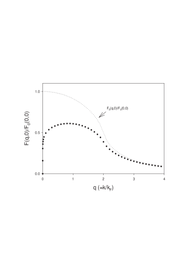
Figure 2: The variational Lindhard function $F(q,0)$(large dotted line) at the zero temperature and frequency; the small dotted line represents the free electron Lindhard function $F_{0}(q,0)$. The magnitudes are renormalized by $F_{0}(0,0)$.

The chemical potential $\mu$ is an independent variable of the thermodynamic potential $\Omega(\mu)$, hence in order to obtain the free energy as a function of electron density, we should change the independent variable using the Legendere transformation; $F(N)=\Omega(\mu)+\mu N$ and $-\frac{\partial\Omega}{\partial\mu}=N$, where $N$ is the number of particles and $F(N)$ is the free energy. However, this relation can not be applied directly in approximations except for Hartree-Fock’s and Baym’s self-consistent schemes [23] because $-\frac{\partial\Omega}{\partial\mu}$ does not represent the particle number. Instead, we use the fact that the Fermi wavevector does not change with the inclusion of correlation according to Luttinger’s theorem [24]. Therefore, we approximate the free energy as follows; $F(N)\simeq\bar{\Omega}_{\rm min}(\mu_{0})+\Delta\Omega_{\rm ring}(\mu_{0})+\mu_{0}N$ and $-\frac{\partial\bar{\Omega}_{\rm min}}{\partial\mu}|_{\mu_{0}}=N$, where the Fermi wavevector (or the density) is fixed by the second relation without the correlation part. In the case of the conventional ring approximation, if $\bar{\Omega}_{\rm min}$ is replaced by a non-interacting part $\Omega_{0}$, the free energy by this transformation reproduces the RPA(random phase approximation) correlation energy.

Figure 3 shows the correlation energy as a function of $r_{s}$ which is the averaged relative distance between electrons defined by $V=(4/3)\pi(a_{0}r_{s})^{3}N$, where $V$, $N$ and $a_{0}$ are the system volume, the number of electrons and the Bohr radius, respectively. The triangles are the result of the Green’s function Monte Carlo calculation [25] and the better agreement with it is realized by the VPT. The conventional rings contain only direct Coulomb interacting processes without exchange contributions which are very important for fermion systems, and thus, the summation of them gives, so called, the RPA result [26]. On the other hand, the variational rings possess infinitely many higher order exchange processes through the variational propagator $G$ as well as direct processes. As a result, we achieve much improvement in the correlation energy beyond the RPA. It is well known that the ring approximation can be applied satisfactorily for very small $r_{s}$ ($r_{s}\ll 1$). In Fig.3, however, we note that even for large $r_{s}$, the variational rings give successful results.

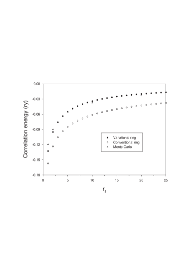
Figure 3: The ground state correlation energy per particle calculated with ring diagrams; the solid and open circles are results of the variational and conventional ring approximations, respectively. The triangles represent the result of the Green’s function Monte Carlo calculation.

Here, we examined the efficiency of the VPT by calculating the correlation energy of the Coulomb electron gas. Further corrections beyond variational rings and the extension to finite temperatures are also easily accessible within the present VPT and we expect good applications to any other systems.

IV summary

After briefly reviewing the VPT formulated recently for the many-particle systems, we have applied this method to the Coulomb electron gas. The ground state correlation energy of the Coulomb electron gas is calculated with the ring approximation of the VPT. Improvement is achieved by the expansion with variational propagators. Especially, we note that even for large $r_{s}$, the approximation produces quite successful results, as is evident from the good agreement with that of the Green’s function Monte Carlo calculation.

- (1) J. Fröhlich, Non-Perturbative quantum field theory (World Scientific, 1992).
- (2) M. C. Gutzwiller, Phys. Rev. Lett. 10, 159 (1963).
- (3) J. D. Talman, Phys. Rev. A 13, 1200 (1976).
- (4) H. S. Noh, S. K. You, and C. K. Kim, Int. J. Mod. Phys. B 11, 1829 (1997).
- (5) J. Bünemann and W. Weber, Phys. Rev. B 55, 4011 (1997).
- (6) A. L. Fetter and J. D. Walecka, Quantum Theory of Many-Particle Systems (McGraw-Hill, 1971).
- (7) G. D. Mahan, Many-Particle Physics (Plenum Press, 1981).
- (8) J. W. Negele and H. Orland, Quantum Many-Particle Systems (Addison-Wesley, 1988).
- (9) P. M. Stevenson, Phys. Rev. D 23, 2916 (1981).
- (10) A. Okopinska, Phys. Rev. D 35, 1835 (1987); 38, 2507 (1988).
- (11) H. Kleinert, Phys. Lett. A 173, 332 (1993).
- (12) V. Janiš, and J. Schlipf, Phys. Rev. B 52, 17119 (1995).
- (13) J. Krzyweck, Phys. Rev. A 56, 4410 (1997).
- (14) M. Bachmann, H. Kleinert, and A. Pelster, Phys. Rev. A 60, 3429 (1999).
- (15) P. Cea and L. Tedesco, Phys. Rev. D 55, 4967 (1997).
- (16) S. K. You, K. J. Jeon, C. K. Kim, and K. Nahm, Eur. J. Phys. 19, 179 (1998).
- (17) S. K. You, C. K. Kim, K. Nahm, and H. S. Noh, Phys. Rev. C 62, 045503 (2000).
- (18) W. F. Lu, C. K. Kim, J. H. Yee, and K. Nahm, Phys. Rev. D 64, 025006 (2001).
- (19) L. S. Schulman, Techniques and Applications of Path Integration (John Wiley and Sons, 1981).
- (20) D. Ruelle, Statistical Mechanics - Rigorous Results (W. A. Benjamin, 1969).
- (21) D. Pines and P. Nozières, The Theory of Quantum Liquids (Addison-Wesley, 1989).
- (22) D. J. Kim, Phys. Rep. 171, 129 (1988).
- (23) G. Baym, Phys. Rev. 127, 1391 (1962).
- (24) J. M. Luttinger, Phys. Rev. 119, 1153 (1960).
- (25) D. M. Ceperley and B. J. Alder, Phys. Rev. Lett. 45, 566 (1980).
- (26) K. S. Singwi, M. P. Tosi, R. H. Land, and A Sjölander, Phys. Rev. 176, 589 (1968).