Symmetry breaking and coarsening of clusters in a prototypical driven granular gas

Abstract

Granular hydrodynamics predicts symmetry-breaking instability in a two-dimensional (2D) ensemble of nearly elastically colliding smooth hard spheres driven, at zero gravity, by a rapidly vibrating sidewall. Super- and subcritical symmetry-breaking bifurcations of the simple clustered state are identified, and the supercritical bifurcation curve is computed. The cluster dynamics proceed as a coarsening process mediated by the gas phase. Far above the bifurcation point the final steady state, selected by coarsening, represents a single strongly localized densely packed 2D cluster.

Introduction. Rapid granular flow continues to attract a great deal of attention of physicists Jaeger . Among most fascinating phenomena here is clustering: nucleation and growth of dense granular clusters, surrounded by dilute granular gas in “freely-cooling” Hopkins and driven Kadanoff1 ; Grossman ; Esipov ; Kudrolli ; Urbach granular gases. Clustering can be viewed as a variant of thermal condensation instability, encountered also in gases and plasmas that cool by their own radiation plasma . This analogy brings about the question of universality of structure formation in ensemble of particles with energy losses of different nature. A related, largely unexplored issue is cluster coarsening. Reviewing different cluster-forming granular systems with a fixed number of particles Hopkins ; Urbach ; Aranson , one notices that coarsening is ubiquitous. In most of these systems a single cluster usually survives after transients die out. The present work addresses novel issues of pattern formation and coarsening in cluster-forming driven granular gases. We shall consider a simple (indeed, prototypical) system: a 2D ensemble of inelastically colliding smooth hard spheres, confined in a rectangular box and driven by a rapidly vibrating side wall at zero gravity. The other three walls are assumed elastic. Though this and related systems were investigated theoretically Kadanoff1 ; Grossman ; Brey ; Tobochnik and experimentally Kudrolli ; Kudrolli2 , it has been recognized only recently that they exhibit nontrivial pattern-forming properties LMS ; KM . These properties will be in the focus of this work. We identify the character of symmetry-breaking bifurcations of the simple clustered state and show that, depending on the control parameters, both super- and subcritical bifurcations can occur. We find that selection of the final steady state occurs via cluster coarsening dynamics, mediated by the gas phase. Far above the bifurcation point, only one densely packed 2D cluster survives. We shall conclude that cluster selection by coarsening is universal in cluster-forming granular flows with a fixed number of particles.

Model. Let $N\gg 1$ identical smooth hard spheres of diameter $d$ and mass $m=1$ are rolling without friction on a smooth horizontal surface of a rectangular box with dimensions $L_{x}\times L_{y}$. The number density of grains is $n(x,y,t)$, the granular temperature is $T(x,y,t)$. For a submonolayer coverage $n\leq n_{c}=2/(\sqrt{3}d^{2})$, the (hexagonal) close-packing density. Three of the walls are immobile, and grain collisions with them are assumed elastic. The fourth wall (located at $x=L_{x}$) is rapidly vibrating, $x=L_{x}+A\cos\omega t$, and supplies energy to the system. The energy is being lost via inelastic hard-core grain collisions characterized by a constant normal restitution coefficient $r$. Our crucial assumption will be a strong inequality $1-r^{2}\ll 1$. In the quasielastic limit, and for small Knudsen numbers, the Navier-Stokes granular hydrodynamics is expected to be reasonably accurate, even for large granular densities, as long as the granulate is in a fluidized state Grossman . Therefore, the steady states of the system can be described by the coarse-grained momentum and energy balance equations

$$p=const\,,\,\,\,\nabla\cdot(\kappa\,\nabla T)=I\,,$$ (1)

where $p$ is the pressure, $\kappa$ is the thermal conductivity and $I$ is the rate of energy losses. To make the full use of hydrodynamics, we shall work in the parameter regime when the energy supply from the vibrating wall can be represented as a hydrodynamic heat flux. This requires $A\ll l$, where $l$ is the mean free path of the particles at the vibrating wall. We shall also assume a double inequality $T^{1/2}/l\ll\omega\ll T^{1/2}/A$. The left inequality guarantees the absence of correlations between successive collisions of particles with the vibrating wall. The right inequality makes the calculation simpler, but it is not crucial. The resulting energy flux is LMS ; Kumaran

$$q=\kappa\,\partial T/\partial x=(2/\pi)^{1/2}\,A^{2}\,\omega^{2}\,n\,T^{1/2}\,.$$ (2)

To close the hydrodynamic model, one needs constitutive relations (CRs) : $p,\kappa$ and $I$ in terms of $n$ and $T$. The CRs have been derived systematically only in the dilute limit. Reasonably accurate CRs in the whole range of densities can be obtained by employing free volume arguments close to the dense-packing limit, interpolating between the high- and low-density limits and finding the fitting constants by comparing the results with particle simulations Grossman ; Luding . We shall use the CRs suggested by Grossman et al. Grossman because of their relative simplicity. A special investigation KM showed that the stability diagram does not change much if one uses instead the CRs derived by Jenkins and Richman JR .

Eqs. (1) can be rewritten in terms of one variable: the (scaled) inverse density $z(x,y)=n_{c}/n(x,y)$ Grossman ; LMS . We introduce scaled coordinates ${\mathbf{r}}/L_{x}\to{\mathbf{r}}$ so that the box dimensions become $1\times\Delta$, where $\Delta=L_{y}/L_{x}$ is the box aspect ratio. We have

$$\nabla\cdot\left(F(z)\nabla z\right)={\cal L}\,Q(z)\,.$$ (3)

Introducing $\psi=\int_{0}^{z}F(z^{\prime})\,dz^{\prime}$, we rewrite it as

$$\nabla^{2}\psi={\cal L}\,\tilde{Q}(\psi)\,$$ (4)

The boundary conditions are

$$\left.\frac{\partial\psi}{\partial x}\right|_{x=0}=\left.\frac{\partial\psi}{\partial y}\right|_{y=0}=\left.\frac{\partial\psi}{\partial y}\right|_{y=\Delta}=0$$ (5)

and (see Ref. LMS )

$$\left.\frac{\partial\psi}{\partial x}\right|_{x=1}={\cal L}\,\tilde{H}\left[\psi(1,y)\right]\,\frac{\int\limits_{0}^{\Delta}\!\int\limits_{0}^{1}\tilde{Q}(\psi)\,dxdy}{\int\limits_{0}^{\Delta}\tilde{H}(\psi(1,y))\,dy}\,.$$ (6)

Here $\tilde{Q}(\psi)=Q\left[z(\psi)\right]$ and $\tilde{H}(\psi)=H\left[z(\psi)\right]$, while $F,G,H$ and $Q$ are functions of $z$ only; they are given in Ref. LMS . In the rest of the paper the symbol  $\tilde{}$  will be omitted. Conservation of the total number of particles yields an equation for the area fraction $f=N/(L_{x}L_{y}n_{c})$:

$$f=\frac{1}{\Delta}\,\int\limits_{0}^{\Delta}\!\int\limits_{0}^{1}\frac{dxdy}{z(\psi)}\,.$$ (7)

The steady state problem is fully determined by three scaled parameters: ${\cal L}=(32/3\gamma)\,(L_{x}/d)^{2}\,(1-r^{2})$ (where $\gamma\simeq 2.26$), the area fraction $f$ and aspect ratio $\Delta$. Notice that the steady-state density distributions are independent of $A$ and $\omega$. This is in contrast to the case of a non-zero gravity, where the gravity acceleration, combined with $A\omega^{2}$, yields a governing parameter.

Strip state. The basic state of the system is the “strip state”: a laterally symmetric cluster located at the wall $x=0$ Grossman . The physics of the strip state is simple. Due to inelastic collisions, the granular temperature goes down with increasing distance from the driving wall. To maintain the pressure balance, the granular density should increase with this distance, reaching the maximum at the opposite (elastic) wall. The strip state is described by the $y$-independent solution of Eqs. (4) and (5); we shall call it $z=Z(x)$ that corresponds to $\psi=\Psi(x)$. Notice that Eq. (6) holds automatically in 1D LMS . An example of the strip state is shown in Fig. 2 (bottom left). A similar state was observed in experiment Kudrolli .

Symmetry-breaking instability. The 1D strip state gives way, by a symmetry-breaking bifurcation, to 2D clustered states. The bifurcation point can be found by linearizing Eqs. (4)-(7) around $\psi=\Psi(x)$. In the framework of time-dependent hydrodynamics, this corresponds to marginal stability of the strip state with respect to small perturbations along the strip. We write

$$\psi(x,y)=\Psi(x)+\varphi_{k}(x)\exp(iky)+\mbox{c.c.}$$ (8)

and, after linearization, arrive at a linear eigenvalue problem for $k=k_{c}(f)$:

$$\varphi_{k}^{\prime\prime}-{\cal L}Q_{\Psi}\,\varphi_{k}-k_{c}^{2}\,\varphi_{k}=0\,,$$ (9)

$$\varphi_{k}^{\prime}(0)=0\,,$$ (10)

$$\varphi_{k}^{\prime}(1)-{\cal L}\,\frac{\int\limits_{0}^{1}\tilde{Q}(\Psi(x))\,dx}{\tilde{H}(\Psi(1))}\,\left.H_{\Psi}\right|_{x=1}\,\varphi_{k}(1)=0\,.$$ (11)

Here and below $(\dots)_{\Psi}(x)=\left.\left[F^{-1}\,d(\dots)/dz\right]\right|_{z=Z(x)}$, and $(\dots)$ stands for any function. Solving the eigenvalue problem for a given ${\cal L}$, we obtain the marginal stability curve $k=k_{c}(f)$ and corresponding eigenfunctions $\varphi_{k}(x)$. The modes with $k<k_{c}(f)$ are unstable. At fixed ${\cal L}$, the instability occurs for $f_{1}({\cal L})<f<f_{2}({\cal L})$, where $k_{c}(f_{1})=k_{c}(f_{2})=0$ LMS . The driving force of the instability is negative effective lateral compressibility of the gas KM . Figure 1 gives an example of the marginal stability curve in terms of the minimum aspect ratio $\Delta_{c}(f)=\pi/k_{c}(f)$, at which the instability occurs.

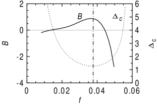
Figure 1: The critical aspect ratio $\Delta$ for the instability and parameter $B$ determining the bifurcation curve (21) versus the area fraction $f$ for ${\cal L}=1.25\cdot 10^{4}$. The vertical dash-dot line corresponds to $f=0.0378$.

Bifurcation curve. To determine the nature of the bifurcation (sub- or supercritical) and compute the bifurcation curve, one should go to the second order of the perturbation theory. We can write

$$\psi(x,y)=\Psi(x)+\sum\limits_{n}\,\varphi_{n}(x)\,\exp(inky)\,,$$ (12)

where $\varphi_{-n}(x)=\varphi^{*}_{n}(x)$, and assume that $\varphi_{0}\sim\varphi_{1}^{2}$, $\varphi_{2}\sim\varphi_{1}^{2}$, $\varphi_{3}\sim\varphi_{1}^{3}$, etc. Therefore, we need to take into account only the terms $n=0,\pm 1$ and $\pm 2$. This yields the following linear equations:

$$\varphi_{0}^{\prime\prime}-{\cal L}\,Q_{\Psi}\,\varphi_{0}={\cal L}\,Q_{\Psi\Psi}\,\left|\varphi\right|^{2}\,,$$ (13)

$$\varphi_{1}^{\prime\prime}-{\cal L}\,Q_{\Psi}\,\varphi_{1}-k_{c}^{2}\varphi_{1}=\left(k^{2}-k_{c}^{2}\right)\,\varphi+$$

$$+{\cal L}\,\left[Q_{\Psi\Psi}\,\left(\varphi_{0}\varphi+\varphi_{2}\varphi^{*}\right)+\frac{1}{2}\,Q_{\Psi\Psi\Psi}\,\varphi\left|\varphi\right|^{2}\right]\,,$$ (14)

$$\varphi_{2}^{\prime\prime}-{\cal L}\,Q_{\Psi}\,\varphi_{2}-4k_{c}^{2}\varphi_{2}=\frac{1}{2}\,{\cal L}\,Q_{\Psi\Psi}\,\varphi^{2}\,,$$ (15)

and the boundary conditions:

$$\varphi_{0}^{\prime}(0)=\varphi_{1}^{\prime}(0)=\varphi_{2}^{\prime}(0)=0\,,$$ (16)

$$\varphi_{1}^{\prime}(1)={\cal L}\Biggl{[}\frac{H_{\Psi}}{H}\varphi_{1}\,\int\limits_{0}^{1}Q\,dx\,$$

$$+\frac{\int\limits_{0}^{1}Q\,dx}{H}\left(H_{\Psi\Psi}\left(\varphi_{0}\varphi+\varphi_{2}\varphi^{*}\right)+\frac{1}{2}H_{\Psi\Psi\Psi}\,\varphi\left|\varphi\right|^{2}\right)$$

$$+\frac{H_{\Psi}}{H}\left(\int\limits_{0}^{1}Q_{\Psi}\,\varphi_{0}\,dx+\int\limits_{0}^{1}Q_{\Psi\Psi}\left|\varphi\right|^{2}\,dx\right)\,\varphi$$

$$-\frac{H_{\Psi}}{H^{2}}\,\varphi\left(H_{\Psi}\,\varphi_{0}+H_{\Psi\Psi}\left|\varphi\right|^{2}\right)\,\int\limits_{0}^{1}Q\,dx\Biggr{]}\Biggr{|}_{x=1}\,,$$ (17)

$$\varphi_{2}^{\prime}(1)={\cal L}\left.\left[\frac{H_{\Psi}}{H}\,\varphi_{2}+\frac{H_{\Psi\Psi}}{2H}\left|\varphi\right|^{2}\right]\right|_{x=1}\,\int\limits_{0}^{1}Q\,dx\,,$$ (18)

where $\varphi=A\,Y(x)$ is a properly normalized solution of Eqs. (9)-(11), see below. As the boundary condition for $\varphi_{0}$ at $x=1$ is fulfilled automatically, one more condition is needed. For a fixed $f$, this condition is supplied by Eq. (7):

$$\int\limits_{0}^{1}\frac{\varphi_{0}}{Z^{2}F}\,dx=2\int\limits_{0}^{1}\left(\frac{1}{Z^{3}F^{2}}+\frac{F_{\Psi}}{2Z^{2}F^{2}}\right)\left|\varphi_{1}\right|^{2}\,dx\,.$$ (19)

The solvability condition for Eq. (14) yields the bifurcation curve: a relation between the amplitude of $\varphi_{1}$ (we call it $A$) and $k_{c}^{2}-k^{2}$. One way to define $A$ is the following: $\varphi_{1}(x)=A\,Y(x)+A|A|^{2}\,\delta\varphi_{1}(x)$, where $Y(x)$ is the solution of Eqs. (9) and (10) obeying the normalization $Y(0)=1$. This yields $A\left(k_{c}^{2}-k^{2}\right)=CA|A|^{2}$, where $C=const$. The trivial solution $A=0$ describes the strip state, while the nontrivial one, $k_{c}^{2}-k^{2}=C|A|^{2}$ describes the bifurcated state. $C>0\,(<0)$ corresponds to supercritical (subcritical) bifurcation. The solvability condition is a generalization of the standard “orthogonality” condition, or the Fredholm alternative Iooss . It yields $C$ explicitly in terms of definite integrals of solutions of the homogeneous forms of Eqs. (9), (13) and (15) that can be found numerically, see Appendix. We present here the resulting bifurcation curve for $Y_{c}$, the (normalized) $y$-coordinate of the center of mass of the granulate:

$$Y_{c}=\frac{\int_{0}^{1}dx\int_{-\Delta/2}^{\Delta/2}\,y\,z^{-1}\,dy}{\Delta\int_{0}^{1}dx\int_{-\Delta/2}^{\Delta/2}z^{-1}\,dy}\,,$$ (20)

where we shifted the $y$-coordinate: $y+\Delta/2\to y$. Let the aspect ratio of the system $\Delta$ be slightly larger than $\Delta_{c}=\pi/k_{c}(f)$ so that only one mode, with $k=\pi/\Delta$, is unstable. The bifurcation curve takes the form

$$\left|Y_{c}\right|=\frac{2}{\pi^{2}B^{1/2}}\left(\frac{\Delta}{\Delta_{c}}-1\right)^{1/2}\,.$$ (21)

where $B=Cf^{2}/(2k_{c}^{2}f_{1}^{2})$ and $f_{1}=2\int_{0}^{1}YZ^{-2}F^{-1}dx$. Eq. (21) assumes $B>0$: a supercritical bifurcation. Figure 1 shows $B(f)$ for ${\cal L}=12,500$. We find that $B>0$ on an interval of $f$ that lies within the instability interval $(f_{1},f_{2})$. Closer to the points $f_{1}$ and $f_{2}$ we obtain $B<0$ which indicates subcritical bifurcation. Subcritical bifurcations close to the high-density instability border were previously observed by solving numerically the nonlinear steady state equations (4)-(6) LMS .

Figure 2: Steady states found in time-dependent hydrodynamic simulations for ${\cal L}=1.25\cdot 10^{4}\,$, $f=0.0378$ and $\Delta=1.2$ (bottom left), $1.3$ (top left) and $3.0$ (right). The left wall of the box is the driving wall.

Time-dependent hydrodynamic simulations: bifurcations and coarsening. We performed a series of time-dependent hydrodynamic simulations, to verify the bifurcation theory and to follow the cluster dynamics at large aspect ratios. The full time-dependent hydrodynamic equations were solved with the same constitutive relations and boundary conditions as those used in our steady state analysis. Instead of the shear viscosity in the Navier-Stokes equation we accounted for a small model friction force $-n{\mathbf{v}}/{\tau}$, where ${\mathbf{v}}$ is the hydrodynamic velocity. An extended version of the compressible hydro code VULCAN vulcan was employed.

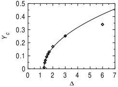
Figure 3: Bifurcation curve $Y_{c}(\Delta)$ predicted by Eq. (21) (line) and found in hydrodynamic simulations (squares) for ${\cal L}=1.25\cdot 10^{4}$ and $f=0.0378$.

We fixed ${\cal L}=1.25\cdot 10^{4}$ and $f=0.0378$ and varied $\Delta$. The initial scaled density included a zero mode corresponding to the fixed $f$ plus small-amplitude random noise. Figure 2 shows the final states for different aspect ratios $\Delta$. For ${\cal L}$ and $f$ used, the marginal stability theory predicts $\Delta_{c}\simeq 1.28$ (see Fig. 1). Indeed, the strip state observed at $\Delta=1.2$ (Fig. 2, bottom left) gives way to a slightly asymmetric state at $\Delta=1.3$ (Fig. 2, top left). Far above the bifurcation point the final state represents a densely packed 2D cluster (“island”), located in a corner (Fig. 2, right). This implies that all but one of the multiple 2D steady state solutions found earlier (chains of islands periodic in the $y$-direction) LMS are unstable. The stable steady state selected by the coarsening dynamics is the one with the maximum possible period, equal to twice the lateral dimension of the system.

Figure 3 shows the bifurcation curve $Y_{c}(\Delta)$ predicted by Eq. (21), and measured in the simulations after transients die out. Excellent agreement is obtained for not too large supercriticalities. Close to the bifurcation point we observed exponential slowdown as expected.

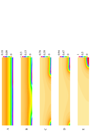
Figure 4: Time history of the density field for ${\cal L}=1.25\cdot 10^{4}$, $f=0.0378$ and $\Delta=5$ at scaled times $650$ (A), $2,100$ (B), $2,850$ (C), $3,250$ (D), and $7,000$ (E). The left wall is the driving wall. Notice the change of color code with time.

Now we present the simulation results on the cluster dynamics and selection. For large $\Delta$ the dynamics involve two stages (see Fig. 4). During the first stage, several clusters nucleate at the wall opposite to the driving wall (Fig. 4A). Their number is of the order of $\Delta/\Delta_{c}$ which apparently corresponds to the maximum linear growth rate of the instability versus $k$. At the slower second stage the clusters become denser. As they compete for the material, their number goes down, and only one densely packed cluster (“island”) finally survives, always in a corner (Fig. 4e). The clusters interact mostly through the gas phase, similarly to Ostwald ripening in phase ordering systems with conserved order parameter, controlled by gasdynamics plasma ; AMS . We also observed, for a different realization of noise in the initial conditions, direct coalescence of transient clusters. However, the resulting single cluster is always the same in simulations with the same ${\cal L},\,f$ and $\Delta$.

In summary, we used hydrodynamics to determine the character of symmetry-breaking bifurcations in a prototypical driven granular gas and compute the supercritical bifurcation curve. We found the selected steady state with broken translational symmetry and showed that selection is made via a coarsening process similar to Ostwald ripening. It appears that cluster selection by coarsening is a universal selection mechanism in cluster-forming granular flows with a fixed number of particles.

This research was supported by the Israel Science Foundation, founded by the Israel Academy of Sciences and Humanities, and by the Russian Foundation for Basic Research (grant No. 02-01-00734).

Appendix. Solvability condition. Here we present the solvability condition for the boundary value problem described by the linear equation (14) and boundary conditions (16) and (17). This solvability conditions yields the constant $C$ that enters the bifurcation equation $k_{c}^{2}-k^{2}=C\,|A|^{2}$. Consider the following problem:

$$w^{\prime\prime}(x)+P(x)w(x) = f(x)\,,$$ (22)

$$w^{\prime}(0) = 0\,,$$ (23)

$$w^{\prime}(1)+aw(1) = g\,,$$ (24)

where $g$ is a parameter; and assume that the homogeneous variant of this problem,

$$w^{\prime\prime}(x)+P(x)w(x) = 0\,,$$ (25)

$$w^{\prime}(0) = 0\,,$$ (26)

$$w^{\prime}(1)+aw(1) = 0$$ (27)

has a nontrivial solution. The problem (22)-(24) will have no solution unless there is a relation between $f(x)$ and $g$. What is the relation? To answer this question, we construct the solution of the problem (22)-(24) using two fundamental solutions $w_{0}$ and $w_{1}$ of the homogeneous equation (25). We choose these solutions as follows. Let $w_{0}$ obeys the boundary conditions  (26) and

$$w_{0}(0)=1\,.$$ (28)

In view of the above assumption, Eq. (27) is fulfilled automatically. The second fundamental solution $w_{1}$ of Eq. (25) obeys the following boundary conditions (again at $x=0$):

$$w_{1}(0)=0\,,\quad w_{1}^{\prime}(0)=1\,.$$ (29)

Notice that each of the solutions $w_{0}$ and $w_{1}$ is defined by an initial value problem, rather than by a boundary value problems.

The general solution of Eqs. (22)-(24) can be written as $C_{0}(x)\,w_{0}(x)+C_{1}(x)\,w_{1}(x)$, where functions $C_{0}(x)$ and $C_{1}(x)$ are yet unknown, and we can demand $C_{0}^{\prime}(x)\,w_{0}(x)+C_{1}^{\prime}(x)\,w_{1}(x)=0$. Straightforward calculations yield the solvability condition

$$g=\left[w_{1}^{\prime}(1)+aw_{1}(1)\right]\int\limits_{0}^{1}fw_{0}\,dx\,.$$ (30)

In the particular case of $g=0$ Eq. (30) is reduced to the standard orthogonality condition $\int\limits_{0}^{1}fw_{0}\,dx\,=0$ Iooss .

Applying the solvability condition (30) to Eq. (14) with the boundary conditions (16) and (17), we obtain the following relationship:

$${\cal L}\Biggl{\{}\left(\frac{H_{\Psi\Psi}}{H}(\varphi_{0}\varphi+\varphi_{2}\varphi^{*})+\frac{H_{\Psi\Psi\Psi}}{2H}\,\varphi\left|\varphi\right|^{2}\right)\int\limits_{0}^{1}Q\,dx+$$

$$+\frac{H_{\Psi}}{H}\varphi\left(\int\limits_{0}^{1}Q_{\Psi}\,\varphi_{0}\,dx+\int\limits_{0}^{1}Q_{\Psi\Psi}\left|\varphi\right|^{2}\,dx\right)-$$

$$-\left(\frac{H_{\Psi}^{2}}{H^{2}}\varphi\varphi_{0}+\frac{H_{\Psi}H_{\Psi\Psi}}{H^{2}}\varphi\left|\varphi\right|^{2}\right)\int\limits_{0}^{1}Q\,dx\Biggr{\}}\Biggr{|}_{x=1}=$$

$$=\left.\left[Y_{11}^{\prime}-{\cal L}\frac{H_{\Psi}}{H}Y_{11}\int\limits_{0}^{1}Q\,dx\right]\right|_{x=1}\int\limits_{0}^{1}Y_{10}\biggl{[}\left(k^{2}-k_{c}^{2}\right)\varphi+$$

$$+{\cal L}\left(Q_{\Psi\Psi}\left(\varphi_{0}\varphi+\varphi_{2}\varphi^{*}\right)+\frac{1}{2}\,Q_{\Psi\Psi\Psi}\,\varphi\left|\varphi\right|^{2}\right)\biggl{]}\,dx\,,$$ (31)

where $Y_{0}(x)$ is solution of Eq. (9) with the boundary conditions

$$Y_{0}(0)=1\,,\quad Y_{0}^{\prime}(0)=0\,,$$ (32)

and $Y_{1}(x)$ is the solution of Eq. (9) with the boundary conditions:

$$Y_{1}(0)=0\,,\quad Y_{1}^{\prime}(0)=1\,.$$ (33)

Notice that each of the solutions $Y_{0}(x)$ and $Y_{1}(x)$ is defined by an initial value problem, rather than by a boundary value problems. This makes the numerical solution straightforward. To complete the calculation, we solve numerically the initial-value problems for the linear differential equations for $\varphi$, $\varphi_{0}$ and $\varphi_{2}$ and compute the definite integrals entering Eqs. (19) and (31). The final result is given by Eq. (21).

References

- (1) H.M. Jaeger, S.R. Nagel, and R.P. Behringer, Rev. Mod. Phys. 68, 1259 (1996); L.P. Kadanoff, Rev. Mod. Phys. 71, 435 (1999).
- (2) M.A. Hopkins and M.Y. Louge, Phys. Fluids A 3, 47 (1991); I. Goldhirsch and G. Zanetti, Phys. Rev. Lett. 70, 1619 (1993); S. McNamara and W.R. Young, Phys. Rev. E 53, 5089 (1996).
- (3) Y. Du, H. Li, and L.P. Kadanoff, Phys. Rev. Lett. 74, 1268 (1995).
- (4) E.L. Grossman, T. Zhou, and E. Ben-Naim, Phys. Rev. E 55, 4200 (1997).
- (5) S.E. Esipov and T. Pöschel, J. Stat. Phys. 86, 1385 (1997).
- (6) A. Kudrolli, M. Wolpert, and J.P. Gollub, Phys. Rev. Lett. 78, 1383 (1997).
- (7) J.S. Olafsen and J.S. Urbach, Phys. Rev. Lett. 81, 4369 (1998).
- (8) B. Meerson, Rev. Mod. Phys. 68, 215 (1996).
- (9) I. S. Aranson et al., Phys. Rev. Lett. 84, 3306 (2000).
- (10) J.J. Brey and D. Cubero, Phys. Rev. E 57, 2019 (1998).
- (11) J. Tobochnik, Phys. Rev. E 60, 7137 (1999).
- (12) A. Kudrolli and J. Henry, Phys. Rev. E 62, R1489 (2000).
- (13) E. Livne, B. Meerson, and P.V. Sasorov, Phys. Rev. E 65, 021302 (2002).
- (14) E. Khain and B. Meerson, cond-mat/0201569.
- (15) V. Kumaran, Phys. Rev. E 57, 5660 (1998).
- (16) S. Luding, Phys. Rev. E 63, 042201 (2001).
- (17) J.T. Jenkins and M.W. Richman, Phys. Fluids 28, 3485 (1985).
- (18) G. Iooss and D.D. Joseph, Elementary Stability and Bifurcation Theory (Springer, New York, 1980), p. 88.
- (19) E. Livne, Astrophys. J. 412, 634 (1993).
- (20) I. Aranson, B. Meerson and P.V. Sasorov, Phys. Rev. E 52, 948 (1995).