The fractality of the relaxation modes in deterministic reaction-diffusion systems

Abstract

In chaotic reaction-diffusion systems with two degrees of freedom, the modes governing the exponential relaxation to the thermodynamic equilibrium present a fractal structure which can be characterized by a Hausdorff dimension. For long wavelength modes, this dimension is related to the Lyapunov exponent and to a reactive diffusion coefficient. This relationship is tested numerically on a reactive multibaker model and on a two-dimensional periodic reactive Lorentz gas. The agreement with the theory is excellent. KEY WORDS:Reaction-diffusion systems; hydrodynamic modes; fractals; microscopic chaos.

PACS numbers: 05.45.Df; 05.45.Ac; 05.60.-k; 05.70.Ln

I Introduction

Recently, many studies have been devoted to fractal structures induced by the chaotic dynamics in the phase-space of non-equilibrium statistical systems and, in particular, to the fractal character of the hydrodynamic modes governing the exponential relaxation of the system to the thermodynamic equilibrium [1, 2, 3, 4, 5, 6, 7, 8, 9, 10, 11, 12] . This fractal character has been related to the entropy production in the approach of equilibrium, for a diffusive multibaker model [1]. Previous works had shown similar results for the entropy production in non-equilibrium steady states [2]. On the other hand, the fractal dimension characterizing the hydrodynamic modes of diffusion has been related to the diffusion coefficient and to the positive Lyapunov exponent by a relation, first obtained for diffusive multibaker maps [3], and proved for general chaotic systems with two degrees of freedom [4]. The construction of the hydrodynamic modes in Refs. [3, 4] gives us a new approach to relate macroscopic transport coefficients and microscopic chaotic properties. It establishes a link between the irreversible transport processes and the reversible microscopic dynamics.

Two other approaches are the so-called escape rate formalism and the thermostated system approach. The first approach can be applied to open systems with absorbing boundaries [5, 6, 7, 8, 9]. The escape of trajectories leads to the formation of a fractal repeller, consisting in the set of orbits forever trapped within the absorbing boundaries. Under such conditions, the transport properties can be related to the positive Lyapunov exponents and the Kolmogorov-Sinai entropy per unit time as well as to fractal dimensions [5, 6, 7, 8, 9]. In the second approach, an external field is applied to the system, and in order to keep the kinetic energy constant, a special force acts on the particles as a heat pump [10, 11, 12]. The system is still time-reversible but does not preserve phase-space volumes anymore. The trajectories converge to a fractal attractor. In thermostated systems, the transport properties have been related to the sum of Lyapunov exponents [11, 12]. In the new approach of Refs. [3, 4], the advantage is that the fractal curve considered is directly related to the hydrodynamic modes of relaxation towards thermodynamic equilibrium. It does not require absorbing boundaries neither a thermostat.

In the present paper, we extend the new approach of Refs. [3, 4] to reaction-diffusion processes. Reaction-diffusion processes are of fundamental importance to understand self-organization in physico-chemical systems [13, 14]. In chemical systems, the microscopic mechanisms of the relaxation toward the thermodynamic equilibrium are still poorly understood already for simple reactions. For the purpose of contributing to this important question, we consider here a simple reactive process of isomerization. The particle is supposed to perform a deterministic motion among static scatterers and to carry a color $A$ or $B$. When colliding on some special scatterers, playing the role of catalysts, its color changes instantaneously with a given probability $p_{0}$,

$$A+\mbox{catalytic\ scatterer}\ \longleftrightarrow \ B+\mbox{catalytic\ scatterer}\ ,\qquad\mbox{with\ probability}\ p_{0}\ ,$$ (1)

$$A+\mbox{other\ scatterer}\ \longleftrightarrow \ A+\mbox{other\ scatterer}\ ,$$ (2)

$$B+\mbox{other\ scatterer}\ \longleftrightarrow \ B+\mbox{other\ scatterer}\ .$$ (3)

For this class of systems, we obtain an expression of the Hausdorff dimension of the reactive modes of relaxation in terms of the reactive dispersion relation and of a function $Q(\alpha,\beta)$ generalizing the Ruelle topological pressure $P(\beta)$. In the long wavelength limit, we then infer a relation between the Hausdorff dimension of the modes, the reactive diffusion coefficient, the reaction rate, and two derivatives of the function $Q(\alpha,\beta)$. In the limit $p_{0}\to 0$, we recover a relation previously derived for the diffusive case [3, 4]. This new expression relates the macroscopic transport and reaction processes to the microscopic underlying dynamics.

The paper is organized as follows. In Section II, we generalize the work of Refs. [4, 3] to the reactive case considered here. In Section III, we test our relation on a reactive multibaker model. We next study the case of a two-dimensional periodic reactive Lorentz gas in Section IV. Conclusions are drawn in Section V.

II Relaxation modes: general results

We consider a system such as a Lorentz gas in which the particles move independently of each other along trajectories of a deterministic dynamical system given by

$$\frac{d{\bf X}}{dt}={\bf F}({\bf X})$$ (4)

The variables of this system are for instance the positions and velocities of the particle: ${\bf X}=({\bf r},{\bf v})$. The vector field ${\bf F}({\bf X})$ is defined in this space. The system is spatially periodic in the positions $\bf r$. The particle moves in a periodic lattice of scatterers given by a certain potential of interaction.

Moreover, each particle carries a color which is either $A$ or $B$. The color changes when the particle interacts with some of the scatterers, called the catalytic scatterers according to the reaction (3). We notice that we may also consider that the particle has a spin one-half which flips upon collision on special scatterers.

We can model the reactive events by a change of color with probability $p_{0}$ when the trajectory meets a certain hypersurface $\Sigma({\bf X})=0$ defined in the space of the variables $\bf X$. This hypersurface surrounds each catalytic scatterer and constitutes the locus where the reaction occurs. The introduction of the color has for consequence that the phase space is composed of two copies of the space of the variables $\bf X$, which are glued together along the hypersurface $\Sigma$. This hypersurface can be viewed as the gate from copy corresponding to the color $A$ to the one corresponding to color $B$ and vice versa. These two copies now form two subspaces of the whole phase space of the reactive system. In this framework, a reactive event corresponds to the crossing of the hypersurface $\Sigma$ from one color subspace to the other.

A statistical ensemble of particles of both colors is described by two probability densities $q({\bf X},A,t)$ and $q({\bf X},B,t)$, to find a particle at the point $\bf X$ with color $c=A$ or $B$, at the current time $t$. The time evolution of these probability densities is ruled by two coupled Liouville equations:

$$\cases{\partial_{t}\;q({\bf X},A,t)+{\rm div}\left[{\bf F}({\bf X})\;q({\bf X},A,t)\right]=-p_{0}\,\Xi\left[\Sigma({\bf X})\right]\left[q({\bf X},A,t)-q({\bf X},B,t)\right]\ ,\cr\partial_{t}\;q({\bf X},B,t)+{\rm div}\left[{\bf F}({\bf X})\;q({\bf X},B,t)\right]=+p_{0}\,\Xi\left[\Sigma({\bf X})\right]\left[q({\bf X},A,t)-q({\bf X},B,t)\right]\ .\cr}$$ (5)

where $\Xi$ is a special distribution defined as

$$\Xi\left[\Sigma({\bf X})\right]\ h({\bf X})\ \equiv\ \lim_{\epsilon\to 0^{+}}\ \left|{\bf F}({\bf X})\cdot\frac{\partial\Sigma}{\partial{\bf X}}({\bf X})\right|\ \delta\left[\Sigma({\bf X})\right]\ h\left[{\bf X}-\epsilon{\bf F}({\bf X})\right]$$ (6)

$\delta$ being the Dirac distribution. The distribution (6) expresses the fact that the particles change their color upon crossing of the hypersurface $\Sigma$. Accordingly, the probability densities just after the hypersurface $\Sigma$ in the direction of the vector field $\bf F$ are the following linear combinations of the densities just before $\Sigma$:

$$\cases{q({\bf X}_{+},A,t)=(1-p_{0})\,q({\bf X}_{-},A,t)+p_{0}\,q({\bf X}_{-},B,t)\ ,\cr q({\bf X}_{+},B,t)=p_{0}\,q({\bf X}_{-},A,t)+(1-p_{0})\,q({\bf X}_{-},B,t)\ ,\cr}$$ (7)

where ${\bf X}_{\pm}={\bf X}_{*}\pm\epsilon{\bf F}({\bf X}_{*})$ with $\Sigma({\bf X}_{*})=0$ and an arbitrarily small $\epsilon>0$. These linear combinations can be expressed in terms of the transmission matrix

$${\mathsf{T}}=\pmatrix{1-p_{0}&p_{0}\cr p_{0}&1-p_{0}\cr}.$$ (8)

We denote by ${\bf X}={\bf\Phi}^{t}{\bf X}_{0}$ the trajectory of the differential equation (4) from the initial condition ${\bf X}_{0}$. Moreover, we gather both probability densities in the vector

$${\bf q}({\bf X},t)=\pmatrix{q({\bf X},A,t)\cr q({\bf X},B,t)\cr}.$$ (9)

The solution of the coupled Liouville equations (5) from the initial probability densities ${\bf q}_{0}$ can then be written in the form of the following Frobenius-Perron operator:

$${\bf q}({\bf X},t)=\left(\hat{\mathsf{P}}^{t}\cdot{\bf q}\right)({\bf X})=\frac{{\mathsf{T}}^{N_{t}({\bf X})}\cdot{\bf q}_{0}\left({\bf\Phi}^{-t}{\bf X}\right)}{\left|\frac{\partial{\bf\Phi}^{t}}{\partial{\bf X}}({\bf\Phi}^{-t}{\bf X})\right|}$$ (10)

with the matrix (8) and where $N_{t}({\bf X})$ is the number of crossings through the hypersurface $\Sigma$ performed by the segment of trajectory from ${\bf X}_{0}={\bf\Phi}^{-t}{\bf X}$ to ${\bf X}={\bf\Phi}^{t}{\bf X}_{0}$. If the flow of Eq. (4) is volume preserving, we have that ${\rm div}{\bf F}=0$ which implies that $\left|\frac{\partial{\bf\Phi}^{t}}{\partial{\bf X}}\right|=1$, which is the case for the systems considered in the following.

The system of Liouville’s equations (5) defines a random process and it is important to characterize the dynamical randomness generated by this process. For this purpose, we calculate its Kolmogorov-Sinai entropy per unit time which is the amount of information produced per unit time by the process. The Kolmogorov-Sinai entropy is calculated by partitioning the whole phase space into small cells and by computing the probability for a trajectory to visit successively different cells of the partition [15]. If we suppose that the differential equation (4) defines a chaotic dynamical system with Lyapunov exponents $\{\lambda_{i}\}$, the dynamical instability of the deterministic motion is a first contribution to the Kolmogorov-Sinai entropy given by the sum of positive Lyapunov exponents according to Pesin’s theorem [15]. A second contribution comes from the random change of color upon crossing of the hypersurface $\Sigma$. At each crossing, the particle jumps from one color subspace to the other with probability $p_{0}$. If the number of crossings is equal to $N_{t}$ during the lapse of time $t$, the frequency of $\Sigma$ crossings is equal to :

$$\nu\ \equiv\ \lim_{t\to\infty}\ \frac{\langle N_{t}\rangle}{t},$$ (11)

where $\langle\cdot\rangle$ denotes the average with respect to the equilibrium state. At each crossing, we have an independent dichotomous random variable with probabilities $(p_{0},1-p_{0})$, which defines a Bernoulli process with the rate $\nu$. Accordingly, the overall Kolmogorov-Sinai entropy per unit time of the process (5) is given by

$$h_{\rm KS}\ =\ \sum_{\lambda_{i}>0}\lambda_{i}\ +\ \nu\ \left[p_{0}\ln\frac{1}{p_{0}}+(1-p_{0})\ln\frac{1}{1-p_{0}}\right].$$ (12)

Pesin’s expression of the Kolmogorov-Sinai entropy is recovered in the deterministic limits $p_{0}=0$ and $p_{0}=1$.

For $0<p_{0}<1$, we remark that the Kolmogorov-Sinai entropy (12) remains positive and finite as for a fully deterministic dynamical system. The way the reaction is modelled here is therefore compatible with a deterministic dynamics that would take place near each catalytic scatterer on a time scale much shorter than the free flight between each scatterer. We can imagine that the reaction follows a complicated trajectory on such a short time scale in a complicated potential, which is here simplified by capturing the complexity of the reaction into a sole transition probability $p_{0}$. Still the so-defined random process has a finite Kolmogorov-Sinai entropy contrary to stochastic processes which have an infinite Kolmogorov-Sinai entropy per unit time. Indeed, it has been shown elsewhere [16, 17] that stochastic processes such as the birth-and-death processes or the linearized Boltzmann processes have a dynamical randomness on arbitrarily small scales $\epsilon$ with an $\epsilon$-entropy per unit time increasing as $h(\epsilon)\sim\ln(1/\epsilon)$. Stochastic processes defined by Langevin stochastic differential equations have an even larger dynamical randomness with an $\epsilon$-entropy per unit time increasing as $h(\epsilon)\sim 1/\epsilon^{2}$. The Kolmogorov-Sinai entropy is the supremum of the $\epsilon$-entropy in the limit $\epsilon\to 0$ and is therefore infinite. In contrast with such stochastic processes, the present random process has a finite Kolmogorov-Sinai entropy. This dynamical randomness is comparable with the randomness of the classical dynamics on graphs which has been recently characterized [18]. For the classical graphs, the motion is one-dimensional so that the only source of randomness is the random bifurcations at the vertices of the graph. Here, there is an extra source of randomness which is the dynamical instability due to the chaotic motion of the particle in the multi-dimensional phase space of Eq. (4).

The overall dynamical randomness (12) induces a relaxation of the probability densities toward the thermodynamic equilibrium. In order to study this relaxation we have to find the relaxation rates which are given by the eigenvalues of the Frobenius-Perron operator (10). It turns out that the Liouville equations (5) can be decoupled if we introduce the probability density $f$ to find a particle at the point $\bf X$ no matter which is its color, and the difference $g$ between both color densities:

$$f({\bf X},t) = q({\bf X},A,t)+q({\bf X},B,t)$$ (13)

$$g({\bf X},t) = q({\bf X},A,t)-q({\bf X},B,t).$$ (14)

These new functions are gathered in the vector

$${\bf q}_{\rm d}({\bf X},t)=\pmatrix{f({\bf X},t)\cr g({\bf X},t)\cr}$$ (15)

which is related to the previous vector (9) by the relation

$${\bf q}_{\rm d}={\mathsf{S}}\cdot{\bf q}$$ (16)

in terms of the matrix

$${\mathsf{S}}=\pmatrix{1&1\cr 1&-1\cr}.$$ (17)

This matrix diagonalizes the transition matrix (8) into

$${\mathsf{T}}_{\rm d}={\mathsf{S}}\cdot{\mathsf{T}}\cdot{\mathsf{S}}^{-1}=\pmatrix{1&0\cr 0&1-2p_{0}\cr}.$$ (18)

Accordingly, the Liouville equations (5) decouple into

$$\cases{\partial_{t}\;f({\bf X},t)+{\rm div}\left[{\bf F}({\bf X})\;f({\bf X},t)\right]=0\ ,\cr\partial_{t}\;g({\bf X},t)+{\rm div}\left[{\bf F}({\bf X})\;g({\bf X},t)\right]=-2p_{0}\,\Xi\left[\Sigma({\bf X})\right]g({\bf X},t)\ .\cr}$$ (19)

which shows that the probability density $f$ obeys the deterministic Liouville equation while the difference $g$ solely controls the reaction. Similarly, the Frobenius-Perron operator (10) splits in the two following operators:

$$f({\bf X},t) = \frac{f_{0}\left({\bf\Phi}^{-t}{\bf X}\right)}{\left|\frac{\partial{\bf\Phi}^{t}}{\partial{\bf X}}({\bf\Phi}^{-t}{\bf X})\right|}$$ (20)

$$g({\bf X},t) = (1-2p_{0})^{N_{t}({\bf X})}\frac{g_{0}\left({\bf\Phi}^{-t}{\bf X}\right)}{\left|\frac{\partial{\bf\Phi}^{t}}{\partial{\bf X}}({\bf\Phi}^{-t}{\bf X})\right|}.$$ (21)

An eigenvalue problem can now be considered separately for both operators (20) and (21). If we denote them generically by $\hat{P}^{t}$, we are looking for eigenstates given by some distributions which are quasiperiodic in the position space $\bf r$ with a wavenumber $\bf k$:

$$\Psi_{\bf k}({\bf X})=e^{i{\bf k}\cdot{\bf r}({\bf X})}\ \Upsilon_{\bf k}({\bf X})$$ (22)

where $\Upsilon_{\bf k}$ is periodic in $\bf r$. The wavenumber $\bf k$ describes spatial inhomogeneities of wavenumber $\ell=2\pi/\|{\bf k}\|$. The distribution (22) is supposed to be a solution of the eigenvalue problem

$$\hat{P}^{t}\Psi_{\bf k}=e^{s_{\bf k}t}\Psi_{\bf k}$$ (23)

associated with the operator $\hat{P}^{t}$. The quantity $-s_{\bf k}$ is the relaxation rate of the eigenstate (22).

The idea is that these eigenstates can be obtained in principle by applying the operator $\hat{P}^{t}$ over a long time to some expression (22) and by renormalizing the result in order to compensate the relaxation according to

$$\Psi_{\bf k}({\bf X})=\lim_{t\to\infty}e^{-s_{\bf k}t}\ \hat{P}^{t}\left[e^{i{\bf k}\cdot{\bf r}({\bf X})}\ \Upsilon({\bf X})\right]$$ (24)

even starting from some arbitrary function $\Upsilon$. This renormalization-semigroup idea has been developed in detail for diffusion in Refs. [17, 24]. For chaotic dynamical systems (4), such eigenstates turn out to be singular distributions without a density function but with cumulative functions defined by

$$F_{\bf k}(\theta)=\int_{0}^{\theta}d\theta^{\prime}\Psi_{\bf k}\left[{\bf X}(\theta^{\prime})\right]$$ (25)

where $\theta$ is a parameter (such as an angle) of a curve ${\bf X}(\theta)$ defined in the phase space.

The hydrodynamic modes of diffusion as well as the reactive modes can be identified as the eigenstates corresponding to the slowest relaxation rates and they can be constructed thanks to the above idea of renormalization semigroup, as we shall show below.

A Diffusive modes

In order to construct a diffusive mode of wavenumber ${\bf k}$ we consider the Frobenius-Perron operator (20) and an initial distribution $\Upsilon({\bf X})$ of particles of initial positions ${\bf r}_{0}$. We integrate the trajectories by using the equations of motion (4) in order to obtain the position ${\bf r}_{t}$ after a long time $t$. As a consequence of the aforementioned idea of renormalization semigroup, the relaxation rate of the diffusive mode is given by the decay rate of the Van Hove intermediate incoherent scattering function [19, 20] as

$$s_{{\bf k}}=\lim_{t\to\infty}\ \frac{1}{t}\ \ln\langle\exp[i{\bf k}\cdot({\bf r}_{t}-{\bf r}_{0})]\rangle$$ (26)

where $\langle\cdot\rangle$ is an average over initial conditions distributed according to some distribution $\Upsilon$ [4, 17, 24]. In a similar way, the cumulative function of the diffusive mode can be obtained as

$$F_{\bf k}(\theta)\equiv\lim_{t\to\infty}\frac{\int_{0}^{\theta}d\theta^{\prime}\ \exp\{i{\bf k}\cdot[{\bf r}_{t}(\theta^{\prime})-{\bf r}_{0}(\theta^{\prime})]\}}{\int_{0}^{2\pi}d\theta^{\prime}\ \exp\{i{\bf k}\cdot[{\bf r}_{t}(\theta^{\prime})-{\bf r}_{0}(\theta^{\prime})]\}}$$ (27)

where the initial conditions are distributed according to a distribution $\Upsilon$ which is here taken as a uniform distribution along a one-dimensional line parametrized by the angle $\theta\;\in[0,2\pi[$ [4].

For two-degree-of-freedom chaotic systems with one positive Lyapunov exponent $\lambda$, the cumulative function (27) forms a fractal curve in the complex plane and its Hausdorff dimension is given in terms of the diffusion coefficient and the Lyapunov exponent according to

$$D_{\rm H}({\bf k})=1+\frac{\cal D}{\lambda}k^{2}+{\mathcal{O}}(k^{4})$$ (28)

as shown in Refs. [3, 4]. The derivation of Ref. [4] is here summarized because we need it for the generalization to the reactive modes.

We assume that we can use the result by Sinai, Bowen and Ruelle that averages can be performed in terms of unstable trajectories covering the phase space within a certain resolution [21, 22, 23]. The probability weight given to each of these trajectories is inversely proportional to their stretching factor $\Lambda_{t}^{(i)}$ which characterizes their dynamical instability. Accordingly, Eq. (26) can be transformed into the condition

$$\sum_{j}|\Lambda_{t}^{(j)}|^{-1}\ \exp(-s_{{\bf k}}t)\ \exp\{i{\bf k}\cdot[{\bf r}_{t}^{(j)}-{\bf r}_{0}^{(j)}]\}\sim_{t\to\infty}\ 1\ .$$ (29)

If the sum in Eq. (29) is restricted to the trajectories issued from initial conditions in the interval $[0,\theta]$, we obtain at time $t$ a polygonal approximation of the cumulative function (27): the integral $\int_{0}^{\theta}$ is an average over trajectories with initial conditions in $[0,\theta]$ and the denominator is proportional to the factor $\exp(s_{\bf k}t)$. At time $t$, the curve $({\rm Re}\;F_{\bf k},{\rm Im}\;F_{\bf k})\subset\hbox{\mb C}$ is thus approximated by a polygon of sides given by the small complex vectors

$$\Delta F^{(j)}=|\Lambda_{t}^{(j)}|^{-1}\;\exp(-s_{\bf k}t)\;\exp\left\{i{\bf k}\cdot\left[{\bf r}_{t}^{(j)}-{\bf r}_{0}^{(j)}\right]\right\}\;.$$ (30)

Each side has the length

$$\varepsilon_{j}=|\Delta F^{(j)}|=|\Lambda_{t}^{(j)}|^{-1}\;\exp(-{\rm Re}\;s_{\bf k}\;t)\;.$$ (31)

In the limit $t\to\infty$, this polygon converges to a fractal curve, characterized by a Hausdorff dimension given by $\sum_{j}\varepsilon_{j}^{D_{\rm H}}\sim 1$. Accordingly, the Hausdorff dimension of the hydrodynamic mode should satisfy the condition

$$\sum_{j}|\Lambda_{t}^{(j)}|^{-D_{\rm H}}\;\exp(-D_{\rm H}\;{\rm Re}\;s_{\bf k}\;t)\sim_{t\to\infty}1\;.$$ (32)

On the other hand, Ruelle’s topological pressure is defined in dynamical systems theory by

$$P(\beta)\equiv\lim_{t\to\infty}\;\frac{1}{t}\;\ln\langle|\Lambda_{t}|^{1-\beta}\rangle$$ (33)

where the average $\langle\cdot\rangle$ is carried out over the equilibrium invariant measure [23]. The mean positive Lyapunov exponent of the system is given by $\lambda=-dP/d\beta|_{\beta=1}$ and in this system without escape, $P(1)=0$. Equation (33) can be transformed into

$$\sum_{j}|\Lambda_{t}^{(j)}|^{-\beta}\;\exp\left[-P(\beta)\;t\right]\sim_{t\to\infty}1\;.$$ (34)

Comparing with Eq. (29), we obtain

$$P(D_{\rm H})=D_{\rm H}\ {\rm Re}\ s_{\bf k}\;.$$ (35)

If the wavenumber ${\bf k}$ vanishes, the cumulative function (27) becomes $F_{{\bf k}=0}(\theta)=\theta/2\pi$, which forms a straight line in the complex plane. In this equilibrium limit, the relaxation rate vanishes, $s_{{\bf k}=0}=0$, so that $P(D_{\rm H})=0$. It means for this system without escape that $D_{\rm H}=1$, as it should be for a straight line. For a non-vanishing but small wavenumber, the Hausdorff dimension is expected to deviate from unity. Inserting $D_{\rm H}=1+\delta$ and the dispersion relation $s_{\bf k}=-{\cal D}k^{2}+{\mathcal{O}}(k^{4})$ in Eq. (35), we can expand both sides in powers of the wavenumber, using the aforementioned properties of the topological pressure. This straightforward calculation shows that the Hausdorff dimension of the hydrodynamic mode is given by Eq. (28) [4].

B Reactive modes

1 General results

We are now going to extend this result to the reactive modes of the isomerization process (3). The modes of interest here are the ones describing the evolution of the difference between the two colors $A$ and $B$, a quantity which relax to zero when the system reaches equilibrium. In this case, we consider the operator (21) which differs from the diffusive Frobenius-Perron operator (20) by the extra factor $(1-2p_{0})^{N_{t}}$. Accordingly, this factor should multiply the exponential $\exp(i{\bf k}\cdot{\bf r})$ in the expression (26) in order to obtain the relaxation rate of the reactive modes, which is thus given by

$$s_{{\bf k}}=\lim_{t\to\infty}\ \frac{1}{t}\ \ln\langle(1-2p_{0})^{N_{t}}\exp[i{\bf k}\cdot({\bf r}_{t}-{\bf r}_{0})]\rangle$$ (36)

where $N_{t}$ is the number of collisions performed on catalysts during the time $t$ [26]. The cumulative function of the reactive modes are similarly given by [26]

$$F_{{\bf k}}(\theta)\equiv\lim_{t\to\infty}\frac{\int_{0}^{\theta}d\theta^{\prime}\ (1-2p_{0})^{N_{t}(\theta^{\prime})}\exp\{i{\bf k}\cdot[{\bf r}_{t}(\theta^{\prime})-{\bf r}_{0}(\theta^{\prime})]\}}{\int_{0}^{2\pi}d\theta^{\prime}\ (1-2p_{0})^{N_{t}(\theta^{\prime})}\exp\{i{\bf k}\cdot[{\bf r}_{t}(\theta^{\prime})-{\bf r}_{0}(\theta^{\prime})]\}}\;.$$ (37)

We notice that Eqs. (36) and (37) consistently reduce to Eqs. (26) and (27) in the purely diffusive limit $p_{0}\to 0$.

As for the diffusive case, Eq. (36) can be transformed into the condition

$$\sum_{j}|\Lambda_{t}^{(j)}|^{-1}\ (1-2p_{0})^{N_{t}^{(j)}}\exp(-s_{{\bf k}}t)\ \exp\{i{\bf k}\cdot[{\bf r}_{t}^{(j)}-{\bf r}_{0}^{(j)}]\}\sim_{t\to\infty}\ 1\;.$$ (38)

The curve $({\rm Re}\;F_{\bf k},{\rm Im}\;F_{\bf k})\subset\hbox{\mb C}$ is approximated at time $t$ by a polygon of sides given by

$$\varepsilon_{j}=|\Delta F^{(j)}|=|\Lambda_{t}^{(j)}|^{-1}\;|1-2p_{0}|^{N_{t}^{(j)}}\;\exp(-{\rm Re}\;s_{\bf k}\;t)\;.$$ (39)

In the limit $t\to\infty$, this polygon converges to a fractal curve, characterized by a Hausdorff dimension given by $\sum_{j}\varepsilon_{j}^{D_{\rm H}}\sim 1$. Accordingly, the Hausdorff dimension of the reactive mode should satisfy the condition

$$\sum_{j}|\Lambda_{t}^{(j)}|^{-D_{\rm H}}\;|1-2p_{0}|^{N_{t}^{(j)}D_{\rm H}}\;\exp(-D_{\rm H}\;{\rm Re}\;s_{\bf k}\;t)\sim_{t\to\infty}1\;.$$ (40)

By analogy with Eq. (34), we can define a function $Q(\alpha,\beta)$ by

$$\sum_{j}|\Lambda_{t}^{(j)}|^{-\beta}\;|1-2p_{0}|^{\alpha N_{t}^{(j)}}\;\exp\left[-Q(\alpha,\beta)t\right]\;\sim_{t\to\infty}1\;$$ (41)

which can be rewritten as

$$Q(\alpha,\beta)=\lim_{t\to\infty}\frac{1}{t}\;\ln\langle(1-2p_{0})^{\alpha N_{t}}\;|\Lambda_{t}|^{1-\beta}\rangle\;.$$ (42)

Comparing Eq. (41) with Eq. (38), we obtain

$$Q(D_{\rm H},D_{\rm H})=D_{\rm H}\ {\rm Re}\ s_{\bf k}\;.$$ (43)

The relation between this new function and the topological pressure is given by

$$P(\beta)=Q(0,\beta)\;.$$ (44)

If the wavenumber ${\bf k}$ vanishes, the cumulative function (37) is reduced to

$$F_{{\bf k}=0}(\theta)=\lim_{t\to\infty}\frac{\int_{0}^{\theta}d\theta^{\prime}(1-2p_{0})^{N_{t}(\theta^{\prime})}}{\int_{0}^{2\pi}d\theta^{\prime}(1-2p_{0})^{N_{t}(\theta^{\prime})}}\;.$$ (45)

This is not a straight line as in the diffusive case: each initial condition is here weighted by a factor $(1-2p_{0})^{N_{t}}$. Provided that $p_{0}<0.5$, this means that the contribution of a given initial condition to $F_{0}$ will be smaller if the corresponding trajectory meets many catalysts, and vice versa. But the Hausdorff dimension of $F_{0}$ is anyway equal to unity. Indeed, for ${\bf k}=0$, the relaxation rate is given by

$$s_{{\bf k}=0}=\lim_{t\to\infty}\frac{1}{t}\;\ln\;\langle(1-2p_{0})^{N_{t}}\rangle,$$ (46)

which is also equal to $Q(1,1)$ according to the definition (42). Using these equalities, we can deduce from (43) that $D_{\rm H}=1$ for vanishing wavenumber. Again the Hausdorff dimension will deviate from unity for a non-vanishing wavenumber. The reactive dispersion relation is given by $s_{\bf k}=-2\kappa-{\cal D}^{\rm(r)}k^{2}+{\mathcal{O}}(k^{4})$. If we compare it with (46) at vanishing wavenumber, we obtain

$$Q(1,1)=-2\kappa=\lim_{t\to\infty}\;\frac{1}{t}\;\ln\langle(1-2p_{0})^{N_{t}}\rangle\;.$$ (47)

Using this equality, the dispersion relation and the expression $D_{\rm H}(k)=1+ak^{2}+{\mathcal{O}}(k^{4})$, Eq. (43) can be expanded in powers of the wavenumber, giving an expression of the Hausdorff dimension of the reactive mode

$$D_{\rm H}({\bf k})=1-\frac{{\cal D}^{\rm(r)}k^{2}}{2\kappa+\frac{\partial Q}{\partial\alpha}(1,1)+\frac{\partial Q}{\partial\beta}(1,1)}+{\mathcal{O}}(k^{4})\;.$$ (48)

An expression for the two partial derivatives of $Q(\alpha,\beta)$ can be directly obtained from Eq. (42), provided that $p_{0}<0.5$:

$$\frac{\partial Q}{\partial\alpha}(1,1)=\ln(1-2p_{0})\ \lim_{t\to\infty}\frac{\langle N_{t}(1-2p_{0})^{N_{t}}\rangle}{t\;\langle(1-2p_{0})^{N_{t}}\rangle}$$ (49)

and

$$\frac{\partial Q}{\partial\beta}(1,1)=-\lim_{t\to\infty}\frac{\langle(1-2p_{0})^{N_{t}}\ln|\Lambda_{t}|\rangle}{t\;\langle(1-2p_{0})^{N_{t}}\rangle}\;.$$ (50)

Similarly, the reactive diffusion coefficient is given by

$${\cal D}^{\rm(r)}=\lim_{t\to\infty}\frac{\langle(1-2p_{0})^{N_{t}}\;({\bf r}_{t}-{\bf r}_{0})^{2}\rangle}{2\;d\;t\;\langle(1-2p_{0})^{N_{t}}\rangle}$$ (51)

where $d$ is the dimension of the space of positions $\bf r$ where diffusion occurs.

2 Limit of small reaction probability $p_{0}\ll 1$

Let us now consider the limit case $p_{0}\ll 1$. The three terms of the denominator appearing in Eq. (48) can be expanded in powers of $p_{0}$. The reaction rate is given by

$$2\kappa = \lim_{t\to\infty}\;\frac{1}{t}\left[\;2\;p_{0}\;\langle N_{t}\rangle+2\;p_{0}^{2}\;\langle N_{t}\rangle+\frac{8}{3}\;p_{0}^{3}\;\langle N_{t}\rangle\right.$$ (54)

$$-2\;p_{0}^{2}\;\left(\langle N_{t}^{2}\rangle-\langle N_{t}\rangle^{2}\right)-4\;p_{0}^{3}\;\left(\langle N_{t}^{2}\rangle-\langle N_{t}\rangle^{2}\right)$$

$$\left.+4\;p_{0}^{3}\;\left(\frac{1}{3}\;\langle N_{t}^{3}\rangle+\frac{2}{3}\;\langle N_{t}\rangle^{3}-\langle N_{t}\rangle\;\langle N_{t}^{2}\rangle\right)+{\mathcal{O}}(p_{0}^{4})\right]$$

$$\iff 2\kappa = 2\;\nu\;p_{0}+2\;(\nu-\sigma^{2})\;p_{0}^{2}+4(\frac{2}{3}\;\nu\;-\;\sigma^{2}\;+\tau)\;p_{0}^{3}+{\mathcal{O}}(p_{0}^{4})$$ (55)

in terms of the frequency (11) of collisions on the catalysts $\nu$ and of the quantities

$$\sigma^{2} = \lim_{t\to\infty}\;\frac{1}{t}\;\left(\langle N_{t}^{2}\rangle-\langle N_{t}\rangle^{2}\right)$$ (56)

$$\tau = \lim_{t\to\infty}\;\frac{1}{t}\;\left(\frac{1}{3}\;\langle N_{t}^{3}\rangle+\frac{2}{3}\;\langle N_{t}\rangle^{3}-\langle N_{t}^{2}\rangle\langle N_{t}\rangle\right)\;.$$ (57)

The two further terms are given by

$$\frac{\partial Q}{\partial\alpha}(1,1) = -\lim_{t\to\infty}\frac{1}{t}\left[2\;p_{0}\;\langle N_{t}\rangle+2\;p_{0}^{2}\;\langle N_{t}\rangle+\frac{8}{3}\;p_{0}^{3}\;\langle N_{t}\rangle\right.$$ (60)

$$-4\;p_{0}^{2}\;\left(\langle N_{t}^{2}\rangle-\langle N_{t}\rangle^{2}\right)-8\;p_{0}^{3}\;\left(\langle N_{t}^{2}\rangle-\langle N_{t}\rangle^{2}\right)$$

$$\left.+12\;p_{0}^{3}\;\left(\frac{1}{3}\;\langle N_{t}^{3}\rangle+\frac{2}{3}\;\langle N_{t}\rangle^{3}-\langle N_{t}^{2}\rangle\;\langle N_{t}\rangle\right)+{\mathcal{O}}(p_{0}^{4})\right]$$

$$\iff\frac{\partial Q}{\partial\alpha}(1,1) = -2\kappa+2\;\sigma^{2}\;p_{0}^{2}+4\;(\sigma^{2}\;-2\;\tau)\;p_{0}^{3}+{\mathcal{O}}(p_{0}^{4})$$ (61)

and

$$\frac{\partial Q}{\partial\beta}(1,1)=-\lambda + 2\;p_{0}\;\lim_{t\to\infty}\;\frac{1}{t}\;C_{\kappa\lambda}(t)$$ (62)

$$+ 2\;p_{0}^{2}\;\lim_{t\to\infty}\;\frac{1}{t}\left[\left(1+2\langle N_{t}\rangle\right)\;C_{\kappa\lambda}(t)-D_{\kappa\lambda}(t)\right]$$ (63)

$$+ 4\;p_{0}^{3}\;\lim_{t\to\infty}\;\frac{1}{t}\left[\left(\frac{2}{3}+2\langle N_{t}\rangle+2\;\langle N_{t}\rangle^{2}-\langle N_{t}^{2}\rangle\right)\;C_{\kappa\lambda}(t)\right.$$ (65)

$$\left.-(1+\langle N_{t}\rangle)\;D_{\kappa\lambda}(t)+\frac{1}{3}E_{\kappa\lambda}(t)\right]+{\mathcal{O}}(p_{0}^{4})$$

$$\iff\frac{\partial Q}{\partial\beta}(1,1) = -\lambda+\alpha_{\kappa\lambda}p_{0}+\beta_{\kappa\lambda}p_{0}^{2}+\gamma_{\kappa\lambda}p_{0}^{3}+{\mathcal{O}}(p_{0}^{4})$$ (66)

where

$$\lambda = \lim_{t\to\infty}\;\frac{1}{t}\;\langle\ln|\Lambda_{t}|\rangle$$ (67)

$$C_{\kappa\lambda}(t) = \langle N_{t}\;\ln|\Lambda_{t}|\rangle-\langle N_{t}\rangle\langle\ln|\Lambda_{t}|\rangle$$ (68)

$$D_{\kappa\lambda}(t) = \langle N_{t}^{2}\;\ln|\Lambda_{t}|\rangle-\langle N_{t}^{2}\rangle\langle\ln|\Lambda_{t}|\rangle$$ (69)

$$E_{\kappa\lambda}(t) = \langle N_{t}^{3}\;\ln|\Lambda_{t}|\rangle-\langle N_{t}^{3}\rangle\langle\ln|\Lambda_{t}|\rangle$$ (70)

$$\alpha_{\kappa\lambda} = 2\;\lim_{t\to\infty}\;\frac{1}{t}\;C_{\kappa\lambda}(t)$$ (71)

$$\beta_{\kappa\lambda} = 2\;\lim_{t\to\infty}\;\frac{1}{t}\left[\left(1+2\langle N_{t}\rangle\right)C_{\kappa\lambda}(t)-D_{\kappa\lambda}(t)\right]$$ (72)

$$\gamma_{\kappa\lambda} = 4\;\lim_{t\to\infty}\;\frac{1}{t}\left[\left(\frac{2}{3}+2\langle N_{t}\rangle+2\;\langle N_{t}\rangle^{2}-\langle N_{t}^{2}\rangle\right)\;C_{\kappa\lambda}(t)\right.$$ (74)

$$\left.-(1+\langle N_{t}\rangle)D_{\kappa\lambda}(t)+\frac{1}{3}E_{\kappa\lambda}(t)\right]\;.$$

For these coefficients, the index $\kappa$ refers to the reaction, related to the number of collisions on a catalyst $N_{t}$, while the index $\lambda$ refers to the dynamical instability, described by the stretching factor $\Lambda_{t}$ and the Lyapunov exponent $\lambda$.

The reactive diffusion coefficient (51) can also be expanded in powers of the reaction probability $p_{0}$ as

$${\cal D}^{(r)}={\cal D}+\Delta\;p_{0}+{\mathcal{O}}(p_{0}^{2})$$ (75)

in terms of the standard diffusion coefficient

$${\cal D}=\lim_{t\to\infty}\frac{1}{2\;d\;t}\;\langle({\bf r}_{t}-{\bf r}_{0})^{2}\rangle$$ (76)

and of the coefficient

$$\Delta=-\;\lim_{t\to\infty}\frac{1}{d\;t}\;\left[\langle N_{t}({\bf r}_{t}-{\bf r}_{0})^{2}\rangle-\langle N_{t}\rangle\langle({\bf r}_{t}-{\bf r}_{0})^{2}\rangle\right]$$ (77)

which characterizes the correlation between the transport by diffusion and the reaction.

We notice that, in the limit $p_{0}\to 0$, the reaction rate (55) vanishes while the reactive diffusion coefficient (51) tends to the diffusion coefficient (76), as expected.

Using (61) and (66), the Hausdorff dimension (48) becomes

$$D_{\rm H}({\bf k}) = 1+\frac{{\cal D}^{\rm(r)}k^{2}}{\lambda\;\left[1-\frac{\alpha_{\kappa\lambda}}{\lambda}\;p_{0}-\frac{\beta_{\kappa\lambda}}{\lambda}\;p_{0}^{2}-\frac{\gamma_{\kappa\lambda}}{\lambda}\;p_{0}^{3}-2\;\frac{\sigma^{2}}{\lambda}\;p_{0}^{2}-4\;\frac{\sigma^{2}}{\lambda}\;p_{0}^{3}+8\;\frac{{\tau}}{\lambda}\;p_{0}^{3}+{\mathcal{O}}(p_{0}^{4})\right]}+{\mathcal{O}}(k^{4})$$ (78)

$$= 1+\frac{{\cal D}^{\rm(r)}k^{2}}{\lambda}\;\left[1+\frac{\alpha_{\kappa\lambda}}{\lambda}\;p_{0}+2\;\frac{\sigma^{2}}{\lambda}\;p_{0}^{2}+\frac{\beta_{\kappa\lambda}}{\lambda}\;p_{0}^{2}+\frac{\alpha_{\kappa\lambda}^{2}}{\lambda^{2}}\;p_{0}^{2}+4\;\frac{\sigma^{2}}{\lambda}\;p_{0}^{3}-8\;\frac{{\tau}}{\lambda}\;p_{0}^{3}\right.$$ (80)

$$\left.+\frac{\gamma_{\kappa\lambda}}{\lambda}\;p_{0}^{3}+2\;\frac{\alpha_{\kappa\lambda}\beta_{\kappa\lambda}}{\lambda^{2}}\;p_{0}^{3}+4\;\frac{\alpha_{\kappa\lambda}\sigma^{2}}{\lambda^{2}}\;p_{0}^{3}+\frac{\alpha_{\kappa\lambda}^{3}}{\lambda^{3}}\;p_{0}^{3}+{\mathcal{O}}(p_{0}^{4})\right]+{\mathcal{O}}(k^{4})\;.$$

or

$$D_{\rm H}({\bf k})=1+\left[\frac{{\cal D}^{\rm(r)}}{\lambda}+{\mathcal{O}}(p_{0})\right]\;k^{2}+{\mathcal{O}}(k^{4})\;.$$ (81)

We immediately see that for $p_{0}\to 0$, Eq. (80) reduces to the expression (28) obtained for the diffusive case.

We are now going to test this formula for two examples: a reactive triadic multibaker and a reactive two-dimensional periodic Lorentz gas.

III The reactive triadic multibaker map

A Description of the model

The multibaker map is a simple model used to mimic a diffusive motion [3, 25]. In the case of the triadic symmetric multibaker, we consider an infinite one-dimensional chain of squares,

$${\mathcal{S}}_{l}=\{(x,y,l):\;0\leq x\leq 1,\;0\leq y\leq 1\}\;,$$ (82)

where $l\in\hbox{\mb Z}$ is the label of the square. A point particle performs jumps from square to square, according to the transition rule $l\to(l-1)$ if $x\leq 1/3$, $l\to l$ if $1/3<x\leq 2/3$ and $l\to(l+1)$ if $x>2/3$. In order to introduce a reaction, the point particle carries a color $A$ or $B$, and the central part $]\frac{1}{3},\frac{2}{3}]$ of one square over $L$ is catalytic: if the point particle is in this portion of the square, it changes its color with a probability $p_{0}$ (see Fig. 1). The map of the model is thus given by

$$\hbox{\boldmath{$\varphi$}}(x,y,l,c)=\cases{(3x,\frac{y}{3},l-1,c)\;,&$0\leq x\leq 1/3$\cr(3x-1,\frac{y+1}{3},l,\varepsilon(l)\;c)\;,&$1/3<x\leq 2/3$\cr(3x-2,\frac{y+2}{3},l+1,c)\;,&$2/3<x\leq 1$\cr}$$ (83)

where $c$ is a discrete variable taking the values $+1$ or $-1$ when the color of the point particle is respectively $A$ or $B$, and

$$\varepsilon(l)=\cases{-1&if $l$ is a catalytic square, with a probability $p_{0}$ ,\cr+1&otherwise .\cr}$$ (84)

We consider the probability density $q(x,y,l,c)$ which evolves under the Frobenius-Perron equation

$$q_{t+1}(x,y,l,c)=\cases{q_{t}\left(\frac{x}{3},3y,l+1,c\right)\;,&$0\leq y\leq 1/3$\cr[1-p_{0}(l)]\;q_{t}\left(\frac{x+1}{3},3y-1,l,c\right)+p_{0}(l)\;q_{t}\left(\frac{x+1}{3},3y-1,l,-c\right)\;,&$1/3<y\leq 2/3$\cr q_{t}\left(\frac{x+2}{3},3y-2,l-1,c\right)\;,&$2/3<y\leq 1$\cr}$$ (85)

where

$$p_{0}(l)=\cases{p_{0}&if $l$ is a catalytic square ,\cr 0&otherwise .\cr}$$ (86)

The Kolmogorov-Sinai entropy per iteration (12) of the reactive triadic multibaker is given by

$$h_{\rm KS}=\ln 3+\frac{p_{0}}{3L}\;\ln\frac{1}{p_{0}}+\frac{1-p_{0}}{3L}\;\ln\frac{1}{1-p_{0}}$$ (87)

because the frequency (11) is equal to the ratio of the area of a reactive rectangle to the area of $L$ squares: $\nu=1/3L$. We notice that the result (87) can also be obtained by using a generating partition which establishes the equivalence between the reactive multibaker map (83) and a Markov chain (see Ref. [17]).

If we define the difference between the densities of the colors $A$ and $B$,

$$g_{t}(x,y,l)=q_{t}(x,y,l,+1)-q_{t}(x,y,l,-1)\;,$$ (88)

we obtain the following equation for its evolution

$$g_{t+1}(x,y,l)=\cases{g_{t}\left(\frac{x}{3},3y,l+1\right)\;,&$0\leq y\leq 1/3$\cr[1-2p_{0}(l)]\;g_{t}\left(\frac{x+1}{3},3y-1,l\right)\;,&$1/3<y\leq 2/3$\cr g_{t}\left(\frac{x+2}{3},3y-2,l-1\right)\;,&$2/3<y\leq 1$\cr}$$ (89)

which is the form of the reactive operator (21) in the case of the present multibaker model.

B Relaxation rates and eigenmodes of the reactive operator

We restrict our description to a unit cell of length $L$, $l=0$ being the catalytic square, and we choose quasiperiodic boundary conditions, assuming that the solution of the equation (89) is quasiperiodic on the chain with a wavenumber $k$. Moreover, we suppose exponentially decaying solutions, with decaying factor $\chi(k)=\exp s_{k}$ where $|\chi(k)|\leq 1$ or ${\rm Re}s_{k}\leq 0$

$$g_{t}(x,y,l)\sim\chi^{t}\;\exp(ikl).$$ (90)

The following operator $\hat{Q}_{k}$ governs the time evolution of $g_{t}(x,y,l)$ [25]:

$$\hat{Q}_{k}\equiv\cases{g_{t+1}(x,y,0)&$=\theta(\frac{1}{3}-y)g_{t}(\frac{x}{3},3y,1)+(1-2p_{0})\theta(y-\frac{1}{3})\theta(\frac{2}{3}-y)g_{t}(\frac{x+1}{3},3y-1,0)$\cr&$+e^{-ikL}\theta(y-\frac{2}{3})g_{t}(\frac{x+2}{3},3y-2,L-1)$\cr g_{t+1}(x,y,1)&$=\theta(\frac{1}{3}-y)g_{t}(\frac{x}{3},3y,2)+\theta(y-\frac{1}{3})\theta(\frac{2}{3}-y)g_{t}(\frac{x+1}{3},3y-1,1)$\cr&$+\theta(y-\frac{2}{3})g_{t}(\frac{x+2}{3},3y-2,0)$\cr&$\vdots$\cr g_{t+1}(x,y,L-2)&$=\theta(\frac{1}{3}-y)g_{t}(\frac{x}{3},3y,L-1)+\theta(y-\frac{1}{3})\theta(\frac{2}{3}-y)g_{t}(\frac{x+1}{3},3y-1,L-2)$\cr&$+\theta(y-\frac{2}{3})g_{t}(\frac{x+2}{3},3y-2,L-3)$\cr g_{t+1}(x,y,L-1)&$=-e^{ikL}\theta(\frac{1}{3}-y)g_{t}(\frac{x}{3},3y,0)+\theta(y-\frac{1}{3})\theta(\frac{2}{3}-y)g_{t}(\frac{x+1}{3},3y-1,L-1)$\cr&$+\theta(y-\frac{2}{3})g_{t}(\frac{x+2}{3},3y-2,L-2)$.\cr}$$ (91)

We now want to obtain the eigenvalues and the eigenstates of this operator

$$\hat{Q}_{k}\{\Psi(x,y,l)\}_{l=0}^{l=L-1}=\chi\{\Psi(x,y,l)\}_{l=0}^{l=L-1}\;.$$ (92)

We suppose that the leading eigenstates are uniform along the unstable direction $x$

$$\Psi(x,y,l)={\mathcal{Y}}(y,l)\;.$$ (93)

If we now cumulate over $x$ and $y$, we get

$$G_{t}(x,y,l)=\int_{0}^{x}dx^{\prime}\int_{0}^{y}dy^{\prime}\Psi(x^{\prime},y^{\prime},l)\equiv x\;C(y,l)$$ (94)

where

$$C(y,l)=\int_{0}^{y}dy^{\prime}{\mathcal{Y}}(y^{\prime},l)$$ (95)

is the reactive cumulative function (37) for the multibaker. We replace $g_{t}(x,y,l)$ by ${\mathcal{Y}}(y,l)$ and $g_{t+1}(x,y,l)$ by $\chi{\mathcal{Y}}(y,l)$ in Eq. (91) and we integrate over the interval $[0,y]$. We obtain

$$C(y,0) = \cases{\frac{1}{3\chi}\;C(3y,1)\;,&$0\leq y\leq 1/3$\cr\frac{1}{3\chi}\;[C(1,1)+(1-2p_{0})C(3y-1,0)]\;,&$1/3<y\leq 2/3$\cr\frac{1}{3\chi}\;[C(1,1)+(1-2p_{0})C(1,0)+e^{-ikL}C(3y-2,L-1)]\;,&$2/3<y\leq 1$\cr}$$ (96)

$$C(y,1) = \cases{\frac{1}{3\chi}\;C(3y,2)\;,&$0\leq y\leq 1/3$\cr\frac{1}{3\chi}\;[C(1,2)+C(3y-1,1)]\;,&$1/3<y\leq 2/3$\cr\frac{1}{3\chi}\;[C(1,2)+C(1,1)+C(3y-2,0)]\;,&$2/3<y\leq 1$\cr}$$ (97)

$$\vdots$$ (98)

$$C(y,L-2) = \cases{\frac{1}{3\chi}\;C(3y,L-1)\;,&$0\leq y\leq 1/3$\cr\frac{1}{3\chi}\;[C(1,L-1)+C(3y-1,L-2)]\;,&$1/3<y\leq 2/3$\cr\frac{1}{3\chi}\;[C(1,L-1)+C(1,L-2)+C(3y-2,L-3)]\;,&$2/3<y\leq 1$\cr}$$ (99)

$$C(y,L-1) = \cases{\frac{e^{ikL}}{3\chi}\;C(3y,0)\;,&$0\leq y\leq 1/3$\cr\frac{1}{3\chi}\;[e^{ikL}\;C(1,0)+C(3y-1,L-1)]\;,&$1/3<y\leq 2/3$\cr\frac{1}{3\chi}\;[e^{ikL}\;C(1,0)+C(1,L-1)+C(3y-2,L-2)]\;,&$2/3<y\leq 1$\cr}.$$ (100)

The eigenvalues are obtained by setting $y=1$ in Eq. (100), which leads to the eigenvalue equation

$$\pmatrix{(1-2p_{0}-3\chi)&1&0&\cdots&0&e^{-ikL}\cr 1&(1-3\chi)&1&\cdots&0&0\cr 0&1&(1-3\chi)&\cdots&0&0\cr\vdots&\vdots&\vdots&\ddots&\vdots&\vdots\cr 0&0&0&\cdots&(1-3\chi)&1\cr e^{ikL}&0&0&\cdots&1&(1-3\chi)\cr}\pmatrix{C(1,0)\cr C(1,1)\cr C(1,2)\cr\vdots\cr C(1,L-2)\cr C(1,L-1)\cr}=0\;.$$ (101)

We thus have to solve the determinant of an Hermitian matrix to find $\chi(k)$. For this purpose, we assume a solution of the form

$$C(1,l)=A\;e^{+i\theta l}+B\;e^{-i\theta l}\;.$$ (102)

After substitution in the system (101), we find that

$$\chi=\frac{1+2\cos\theta}{3}$$ (103)

and

$$\cos kL=\cos\theta L+p_{0}\;\frac{\sin\theta L}{\sin\theta}.$$ (104)

For the present reactive system, the relaxation rate $s(k)=\ln\chi(k)$ depends on the wavenumber $k$ as $s(k)=-2\kappa-{\cal D}^{\rm(r)}k^{2}+{\mathcal{O}}(k^{4})$, where $\kappa$ is the reaction rate and ${\cal D}^{\rm(r)}$ is the reactive diffusion coefficient.

Solving Eq. (104) for its leading root, we can thus obtain the reaction rate and the reactive diffusion coefficient either in powers of the transition probability $p_{0}$:

$$\kappa = \frac{p_{0}}{3L}+\left(\frac{1}{L^{2}}-\frac{1}{3}\right)\frac{p_{0}^{2}}{6}+{\mathcal{O}}(p_{0}^{3})\;,$$ (105)

$${\cal D}^{\rm(r)} = \frac{1}{3}+\frac{2p_{0}}{9L}+{\mathcal{O}}(p_{0}^{2})\;,$$ (106)

or in the asymptotic limit $L\to\infty$:

$$\kappa = \frac{\pi^{2}}{6L^{2}}-\frac{2\pi^{2}}{3p_{0}L^{3}}+{\mathcal{O}}\left(\frac{1}{L^{4}}\right)\;,$$ (107)

$${\cal D}^{\rm(r)} = \frac{\pi^{2}}{3p_{0}L}+{\mathcal{O}}\left(\frac{1}{L^{2}}\right)\;.$$ (108)

In the limit $p_{0}\to 0$, Eq. (105) shows that the reaction rate vanishes linearly with the transition probability and Eq. (106) that the reactive diffusion coefficient tends to the purely diffusive one ${\cal D}=1/3$, as expected. On the other hand, Eq. (107) shows that the reaction rate decreases as $L^{-2}$ when the catalytic sides are diluted in the limit $L\to\infty$, as expected for a diffusion-controled reaction in a one-dimensional system [25]. Moreover, the vanishing of the reactive diffusion coefficient (108) as $L^{-1}$ for $L\to\infty$ is consistent with the results previously obtained in Ref. [25]. We notice the remarkable property that, in the diffusion-controled regime of the reaction, the leading term of the asymptotic expression for the reaction rate (107) does not depend on the transition probability $p_{0}$, which only appears in the next terms. Therefore, the leading term of (107) no longer expresses the property that the reaction rate vanishes in the limit $p_{0}\to 0$, as shown by Eq. (105). This is consistent with the fact that the reaction rate is largely independent of the local reaction rate at the catalysts in the diffusion-controled regime, as already noticed in Refs. [9, 26].

Let us consider more explicitly the simple case $L=1$. In this case, Eq. (101) reduces to

$$3\chi-2\cos k-1+2p_{0}=0$$ (109)

which gives the solution

$$\chi(k)=\frac{1-2p_{0}+2\cos k}{3}\;.$$ (110)

For $k\ll 1$, $\chi(k)$ is then given by

$$\chi(k) \simeq e^{-2\kappa}e^{-{\cal D}^{\rm(r)}k^{2}}$$ (111)

$$\simeq \chi_{0}\;(1-{\cal D}^{\rm(r)}k^{2})\;.$$ (112)

Expanding (110) in powers of $k$ up to the second degree, we obtain

$$\chi\simeq\frac{3-2p_{0}}{3}\;\left(1-\frac{1}{3-2p_{0}}k^{2}\right)$$ (113)

which allows us to identify $\chi_{0}=\frac{3-2p_{0}}{3}=e^{-2\kappa}$ and ${\cal D}^{\rm(r)}=\frac{1}{3-2p_{0}}$.

The dependence of the reactive diffusion coefficient ${\cal D}^{\rm(r)}$ on $p_{0}$ is shown in Fig. 2 for different values of the chain length $L$. The value of the diffusion coefficient $\cal D$ is indicated for comparison.

C Fractal dimension of the cumulative functions of the eigenmodes

We now want to study the cumulative functions $C(y,l)$, solutions of Eq. (100), and more specifically to calculate their dimension. These functions are represented in the complex plane in the case $L=1$ in Figs. 3 and 4. Fig. 3 shows their dependence on the reaction probability $p_{0}$, the wavenumber being fixed, $k=0.1$. Their dependence on the wavenumber for $p_{0}=0.3$ is shown in Fig. 4. As explained in Section II, these complex cumulative functions can be approximated by a polygon at a given time $t$, which means at a certain iteration step $n$ in this discrete case. This concept will here be applied using a symbolic dynamics.

The symbolic dynamics is constructed by partitioning the phase space of the multibaker maps depicted in Fig. 1. Each of the $L$ squares of the chain is divided in three parts for $x\in[0,\frac{1}{3}]$, $x\in]\frac{1}{3},\frac{2}{3}]$ or $x\in]\frac{2}{3},1]$. These $3L$ rectangles are successively assigned the symbols $\omega_{n}\in\{0,1,\cdots,3L-2,3L-1\}$ from left to right along the chain. At the $n^{\rm th}$ step of the construction described in Subsection II B, the cumulative function is a polygon in the complex plane with its sides corresponding to a subrectangle associated with a sequence of $n$ symbols $\{\omega_{n-1}\omega_{n-2}\cdots\omega_{1}\omega_{0}\}$. Moreover, we notice that the sequence of symbols also determines the square $l$ where the point is located along the chain. At the next steps of the construction, the cumulative function keeps its values already obtained at the borders of each of the aforementioned subrectangles. We can thus denote the values of the cumulative function at the lower and upper borders $y_{\pm}(\omega_{n-1},\omega_{n-2},\cdots,\omega_{1},\omega_{0})$ of one of the subrectangles in the square $l$ more shortly by

$$C_{\pm}(\omega_{n-1},\omega_{n-2},\dots,\omega_{1},\omega_{0})=C\left[y_{\pm}(\omega_{n-1},\omega_{n-2},\dots,\omega_{1},\omega_{0}),l\right].$$ (114)

The complex vector defining the side of the polygon at the $n^{\rm th}$ step of the construction is thus given by

$$\Delta C(\omega_{n-1},\omega_{n-2},\dots,\omega_{1},\omega_{0})=C_{+}(\omega_{n-1},\omega_{n-2},\dots,\omega_{1},\omega_{0})-C_{-}(\omega_{n-1},\omega_{n-2},\cdots,\omega_{1},\omega_{0}).$$ (115)

The succession of two symbols $\omega_{1}\omega_{0}$ corresponds to a transition in the multibaker phase-space, with which a certain probability is associated . Using (100), we can construct a $3L\times 3L$ transition matrix $\mathsf{M}$ of elements $M_{\omega_{1}\omega_{0}}$ describing the factor connecting the portion of square corresponding to $\omega_{0}$ to the one corresponding to $\omega_{1}$. Using this matrix, we can describe the time evolution of the intervals $\Delta C(\omega_{n-1},\omega_{n-2},\dots,\omega_{1},\omega_{0})$ as

$$\Delta C(\omega_{n-1},\omega_{n-2},\dots,\omega_{1},\omega_{0})=M_{\omega_{n-1}\omega_{n-2}}M_{\omega_{n-2}\omega_{n-3}}\cdots M_{\omega_{2}\omega_{1}}M_{\omega_{1}\omega_{0}}\Delta C(\omega_{0})\;.$$ (116)

We define

$$\Gamma_{n}^{D}(C) = \sum_{\omega_{0}\cdots\omega_{n-1}}\left|\Delta C(\omega_{n-1},\omega_{n-2},\dots,\omega_{1},\omega_{0})\right|^{D}$$ (117)

$$= \sum_{\omega_{0}\cdots\omega_{n-1}}\left|M_{\omega_{n-1}\omega_{n-2}}\right|^{D}\cdots\left|M_{\omega_{1}\omega_{0}}\right|^{D}\left|\Delta C(\omega_{0})\right|^{D}$$ (118)

$$= \sum_{\omega_{0}\omega_{n-1}}({\mathcal{M}}^{n-1})_{\omega_{n-1}\omega_{0}}\left|\Delta C(\omega_{0})\right|^{D}$$ (119)

where the matrix $\mathcal{M}$ is composed of the elements:

$${\mathcal{M}}_{\omega\omega^{\prime}}=\left|M_{\omega\omega^{\prime}}\right|^{D}\;.$$ (120)

Supposing that this matrix admit the spectral decomposition, ${\mathcal{M}}=\sum_{\mu}|\mu\rangle\;\mu\;\langle\mu|$, Eq. (119) can be rewritten as

$$\Gamma_{n}^{D}(C)=\sum_{\mu}\;\langle{\bf u}|\mu\rangle\;\mu^{n-1}\;\langle\mu|{\bf v}\rangle$$ (121)

where $\bf u$ denotes the vector of unit elements $u_{\omega}=1$ and $\bf v$ the vector with the elements $v_{\omega}=|\Delta C(\omega)|^{D}$. According to the definition of the Hausdorff dimension, for $n\to\infty$, the quantity (121) must converge to a finite non-vanishing value if $D=D_{\rm H}$. This will only be the case if $\mu=1$. $D_{\rm H}$ is thus solution of the equation obtained by imposing $1$ as eigenvalue of the matrix ${\mathcal{M}}$. Let us consider explicitly the case $L=1$. We have to calculate the $3\times 3$ determinant

$$\left|\matrix{\left|\frac{1}{3\chi}\right|^{D_{\rm H}}-1&\left|\frac{1}{3\chi}\right|^{D_{\rm H}}&\left|\frac{1}{3\chi}\right|^{D_{\rm H}}\cr\left|\frac{1-2p_{0}}{3\chi}\right|^{D_{\rm H}}&\left|\frac{1-2p_{0}}{3\chi}\right|^{D_{\rm H}}-1&\left|\frac{1-2p_{0}}{3\chi}\right|^{D_{\rm H}}\cr\left|\frac{1}{3\chi}\right|^{D_{\rm H}}&\left|\frac{1}{3\chi}\right|^{D_{\rm H}}&\left|\frac{1}{3\chi}\right|^{D_{\rm H}}-1\cr}\right|=0.$$ (122)

This gives the equation

$$\left(\frac{1-2p_{0}}{3\chi}\right)^{D_{\rm H}}+2\left(\frac{1}{3\chi}\right)^{D_{\rm H}}-1=0\;.$$ (123)

We will solve (123) in the limit case $p_{0}\to 0$, using the expression of $\chi$ in the case $L=1$ (110). For $p_{0}=0$, we have $D_{\rm H}^{(0)}=\frac{\ln 3}{\ln(1+2\cos k)}$. On the other hand, the Hausdorff dimension takes the unit value for $k=0$. Substituting the expansion $D_{\rm H}=1+ak^{2}+{\cal O}(k^{4})$ in Eq. (123) and expanding in powers of the wavenumber $k$, we can solve for the unknown coefficient $a$ and obtain

$$D_{\rm H}=1+\frac{k^{2}}{(3-2p_{0})\ln(3-2p_{0})-(1-2p_{0})\ln(1-2p_{0})}+{\cal O}(k^{4})\;.$$ (124)

Now expanding in powers of the transition probability $p_{0}$, we finally obtain

$$D_{\rm H}=1+\frac{1}{\ln 3}\;\frac{1}{3}\left(1+\frac{2}{3}p_{0}+\frac{4}{9}p_{0}^{2}+\frac{8}{27}p_{0}^{3}\right)k^{2}+\frac{1}{(\ln 3)^{2}}\left(\frac{4}{27}p_{0}^{2}+\frac{80}{243}p_{0}^{3}\right)\;k^{2}+{\mathcal{O}}(p_{0}^{4}k^{2})+{\mathcal{O}}(k^{4})$$ (125)

We can again compare this expression with the general result (80) of Section II. For the triadic multibaker, the Lyapunov exponent is given by $\lambda=\ln 3$. Moreover, the stretching factor $\ln|\Lambda_{t}|$ is constant in the triadic multibaker, which implies that the coefficients $C_{\kappa\lambda}$, $D_{\kappa\lambda}$, $E_{\kappa\lambda}$ and therefore $\alpha_{\kappa\lambda}$, $\beta_{\kappa\lambda}$, $\gamma_{\kappa\lambda}$ defined in Eqs. (68)-(74) are vanishing. Whereupon, Eq. (80) is here reduced to

$$D_{\rm H}(k)=1+\frac{{\cal D}^{\rm(r)}k^{2}}{\lambda}\;\left[1+2\;\frac{\sigma^{2}}{\lambda}\;p_{0}^{2}+4\;\frac{\sigma^{2}}{\lambda}\;p_{0}^{3}-8\;\frac{{\tau}}{\lambda}\;p_{0}^{3}+{\mathcal{O}}(p_{0}^{4})\right]+{\mathcal{O}}(k^{4})\;.$$ (126)

Using the expansion of the reactive diffusion coefficient up to the third order in $p_{0}$

$${\cal D}^{\rm(r)}=\frac{1}{3}\left[1+\frac{1}{3}p_{0}+\frac{4}{9}p_{0}^{2}+\frac{8}{27}p_{0}^{3}+{\mathcal{O}}(p_{0}^{4})\right]\;,$$ (127)

Eq. (126) becomes

$$D_{\rm H}(k) = 1+\frac{1}{\ln 3}\;\frac{1}{3}\left(1+\frac{1}{3}p_{0}+\frac{4}{9}p_{0}^{2}+\frac{8}{27}p_{0}^{3}\right)k^{2}+\frac{1}{(\ln 3)^{2}}\left(\frac{1}{3}+\frac{2}{9}\;p_{0}\right)\;2\sigma^{2}\;p_{0}^{2}\;k^{2}$$ (129)

$$+\frac{1}{(\ln 3)^{2}}\frac{1}{3}\;4\;\sigma^{2}\;p_{0}^{3}\;k^{2}-\frac{1}{(\ln 3)^{2}}\;\frac{1}{3}\;8\;\tau\;p_{0}^{3}\;k^{2}+{\mathcal{O}}(p_{0}^{4}k^{2})+{\mathcal{O}}(k^{4})\;.$$

The second term of the right members of (125) and (129) are equal. They correspond to $\frac{{\cal D}^{\rm(r)}k^{2}}{\lambda}$. Let us now compare the other corrections in $p_{0}$. The only correction in $p_{0}^{2}$ in (129) is $\frac{1}{(\ln 3)^{2}}\;\frac{1}{3}\;2\;\sigma^{2}\;p_{0}^{2}\;k^{2}$. We can evaluate $\sigma^{2}=\lim_{t\to\infty}\;\frac{1}{t}\;(\langle N_{t}^{2}\rangle-\langle N_{t}\rangle^{2})$ in the case of the triadic reactive multibaker $L=1$. Indeed here, colliding on a catalyst corresponds to being in the region $x\in]\frac{1}{3},\frac{2}{3}]$. The mean number of collisions on a catalyst per unit time is then

$$\frac{1}{t}\;\langle N_{t}\rangle=\frac{1}{3}\cdot 0+\frac{1}{3}\cdot 1+\frac{1}{3}\cdot 0=\frac{1}{3}$$ (130)

and

$$\frac{1}{t}\;\langle N_{t}^{2}\rangle=\frac{1}{3}\cdot 0^{2}+\frac{1}{3}\cdot 1^{2}+\frac{1}{3}\cdot 0^{2}=\frac{1}{3}$$ (131)

which finally gives us

$$\sigma^{2}=\frac{1}{3}-\left(\frac{1}{3}\right)^{2}=\frac{2}{9}\;.$$ (132)

The coefficient of the correction in $p_{0}^{2}$ is then equal to $\frac{1}{(\ln 3)^{2}}\;\frac{4}{27}$, which is exactly the coefficient obtained in (125). The correction in $p_{0}^{3}$ in (129) contains three different contributions: $\frac{1}{(\ln 3)^{2}}\frac{4}{9}\;\sigma^{2}\;p_{0}^{3}\;k^{2}+\frac{1}{(\ln 3)^{2}}\frac{4}{3}\;\sigma^{2}\;p_{0}^{3}\;k^{2}-\frac{1}{(\ln 3)^{2}}\;\frac{8}{3}\;\tau\;p_{0}^{3}\;k^{2}$. Again we can evaluate $\tau$

$$\tau = \lim_{t\to\infty}\;\frac{1}{t}\;\left(\frac{1}{3}\;\langle N_{t}^{3}\rangle+\frac{2}{3}\;\langle N_{t}\rangle^{3}-\langle N_{t}^{2}\rangle\langle N_{t}\rangle\right)$$ (133)

$$= \frac{1}{3}\cdot\frac{1}{3}+\frac{2}{3}\cdot\frac{1}{27}-\frac{1}{3}\cdot\frac{1}{3}=\frac{2}{81}\;.$$ (134)

We obtain $\frac{1}{(\ln 3)^{2}}\frac{80}{243}$, which is the coefficient expected for the correction in $p_{0}^{3}$. Accordingly, we have confirmed that Eq. (80) for the Hausdorff dimension of the reactive modes is valid for the reactive multibaker map. The validity of the approach is furthermore tested in Fig. 5, where the Hausdorff diemansion $D_{\rm H}$ is plotted versus the square of the wavenumber $k^{2}$. The symbols are obtained numerically by solving Eq. (123) and compared with the expression (125). The agreement is good up to $p_{0}=0.3$. We notice that, beyond this value, further terms would be required in the Taylor expansion (125).

IV The 2D reactive periodic Lorentz gas

We are now going to consider as second example a two-dimensional reactive periodic Lorentz gas. This model has been introduced in Ref. [26]. In this system, a point particle, carrying a color $A$ or $B$ undergoes elastic collisions on hard disks fixed in the plane and forming a regular triangular lattice characterized by the lattice fundamental vectors ${\bf e}_{1}=d(1,0)$ and ${\bf e}_{2}=d(\frac{1}{2},\frac{\sqrt{3}}{2})$. The radius of the disks is assumed to be equal to unity and $d$ is the distance between their centers. We shall work in the finite horizon regime, $2<d<\frac{4}{\sqrt{3}}$, for which the diffusion coefficient is finite. Some of the disks play the role of catalysts: when the point particle collides on one of them, it changes its color instantaneously with a probability $p_{0}$. The catalysts form a regular triangular superlattice over the disks lattice, with as fundamental vectors ${\bf E}_{1}=nd(0,-\sqrt{3})$ and ${\bf E}_{2}=nd(\frac{3}{2},\frac{\sqrt{3}}{2})$, where $n$ is an integer parameter controlling the density of catalysts: in the direction of ${\bf E}_{1}$ and ${\bf E}_{2}$, one disk over $n$ is a catalyst. Globally, one disk over $N=3n^{2}$ is a catalyst. The configurations with $n=1$ and $n=2$ are depicted in Fig. 6.

Our goal here is to study the cumulative reactive eigenfunctions of this system. As done in Ref. [26], we will construct the Frobenius-Perron operator governing the time evolution of the color density describing the reactive process in this system. We will then perform a spectral analysis of this operator.

A The reactive operator

The variables needed to describe the point particle in this system are its position, its velocity and its color, i.e. $(x,y,v_{x},v_{y},c)$, where $c$ is a discrete variable taking the values $+1$ or $-1$ when the particle color is $A$ or $B$. However, the collisions on the disks being elastic, the energy of the point particle is conserved. The magnitude of its velocity is a constant of motion, that we suppose equal to one, $\|{\bf v}\|=1$. The velocity can therefore be described by only one coordinate, which can be for example the angle between the velocity and the $x$-axis. This system is periodic, which means that instead of describing the dynamics in the full space, we can restrict our description to an elementary cell of the superlattice of catalysts, containing $N$ disks (see Fig. 6). Moreover, the relevant information concerning the dynamics is contained in the collision dynamics: between two collisions, the point particle performs a free flight. The three-dimensional flow dynamics can therefore be reduced to a Poincaré-Birkhoff map, describing the dynamics from collision to collision. We will use the Birkhoff coordinates ${\bf x}=(j,\theta,\varpi)$, $1\leq j\leq N=3n^{2}$, $0\leq\theta<2\pi$, $-1\leq\varpi\leq 1$, where $j$ is the index of the disk of the elementary cell on which the collision takes place, $\theta$ is an angle giving the position of the impact on this disk and $\varpi$ is the sine of the angle between the outgoing velocity and the normal at the impact. In these coordinates, the mapping of the reactive Lorentz gas is given by

$$\cases{{\bf x}_{n+1}=\hbox{\boldmath{$\varphi$}}({\bf x}_{n})\ ,\cr t_{n+1}=t_{n}+T({\bf x}_{n})\ ,\cr{\bf l}_{n+1}={\bf l}_{n}+{\bf a}({\bf x}_{n})\ ,\cr c_{n+1}=\varepsilon({\bf x}_{n})\ c_{n}\ .\cr}$$ (135)

$t_{n}$ is the time of the $n^{\rm th}$ collision. $T({\bf x})$ is the first-return time function. The vector ${\bf l}_{n}$ gives the cell of the superlattice visited at time $t_{n}$ and ${\bf a}({\bf x}_{n})$ is a vector giving the jump carried out on the superlattice during the free flight from ${\bf x}_{n}$ to ${\bf x}_{n+1}$. The change of color is controlled by the function:

$$\varepsilon({\bf x}_{n})=\cases{-1&if $j_{n}$ is a catalyst, with a probability $p_{0}$ ,\cr+1&otherwise .\cr}$$ (136)

We notice that the dynamical randomness of the reactive Lorentz gas is characterized by the following Kolmogorov-Sinai entropy per unit time

$$h_{\rm KS}\ =\ \lambda\ +\ \nu\ \left[p_{0}\ln\frac{1}{p_{0}}+(1-p_{0})\ln\frac{1}{1-p_{0}}\right]$$ (137)

where $\lambda$ is the unique positive Lyapunov exponent of the two-dimensional Lorentz gas and $\nu$ is the frequency of encounters with a catalytic disk.

We now want to obtain the Frobenius-Perron operator associated with this map. We first start from a description of the particle in the full space. The current state and position of the particle are given by a suspended flow in terms of the coordinates $({\bf x},\tau,{\bf l},c)$, where $0\leq\tau<T({\bf x})$ is the time elapsed since the last collision, ${\bf l}$ is a vector of the superlattice and $c=\pm 1$. The phase-space probability density depending on these variables $q({\bf x},\tau,{\bf l},c)$ evolves in time under the Frobenius-Perron operator defined by Eq. (10) [26]. This continuous-time operator can be reduced to an operator describing the dynamics from collision to collision under the mapping (135). The details are presented in Ref. [26]. The operator for the modes of wavenumber ${\bf k}$ is given by

$$\hat{R}_{{\bf k},s}\ \tilde{q}_{{\bf k},s}({\bf x},c) = \exp[-sT(\hbox{\boldmath{$\varphi$}}^{-1}{\bf x})-i{\bf k}\cdot{\bf a}(\hbox{\boldmath{$\varphi$}}^{-1}{\bf x})]$$ (139)

$$\times\ \{[1-p(\hbox{\boldmath{$\varphi$}}^{-1}{\bf x})]\tilde{q}_{{\bf k},s}(\hbox{\boldmath{$\varphi$}}^{-1}{\bf x},c)\ +\ p(\hbox{\boldmath{$\varphi$}}^{-1}{\bf x})\ \tilde{q}_{{\bf k},s}(\hbox{\boldmath{$\varphi$}}^{-1}{\bf x},-c)\}$$

where

$$p({\bf x}=\{j,\theta,\varpi\})=\cases{p_{0}&if $j$ is a catalyst,\cr 0&otherwise.\cr}$$ (140)

The operator $\hat{R}_{k,s}$ is similar to a Frobenius-Perron operator of the mapping $\varphi$ up to important factors which take into account the varying time of flight between the collisions, the spatial modulation by the wavenumber $\bf k$, as well as the color change on a part of the domain of definition of the Poincaré-Birkhoff mapping. If we now consider the total phase-space density $f({\bf x})=\tilde{q}({\bf x},A)+\tilde{q}({\bf x},B)$ and the difference of phase-space densities $g({\bf x})=\tilde{q}({\bf x},A)-\tilde{q}({\bf x},B)$, their time evolutions are decoupled and we can write an operator governing the evolution of $g({\bf x})$, describing the reactive modes of wavenumber ${\bf k}$ in this system [26]

$$\hat{W}_{{\bf k},s}\ g({\bf x})=[1-2p(\hbox{\boldmath{$\varphi$}}^{-1}{\bf x})]\ \exp[-sT(\hbox{\boldmath{$\varphi$}}^{-1}{\bf x})-i{\bf k}\cdot{\bf a}(\hbox{\boldmath{$\varphi$}}^{-1}{\bf x})]\ g(\hbox{\boldmath{$\varphi$}}^{-1}{\bf x})\ ,$$ (141)

which we call the reactive operator.

B Spectral analysis of the reactive operator

To identify the eigenmode of the reactive operator (141) which controls the slowest relaxation of the color, we consider the eigenvalue problem for $\hat{W}_{{\bf k},s_{\bf k}}$ and its adjoint $\hat{W}_{{\bf k},s_{\bf k}}^{{\dagger}}$ imposing $1$ as eigenvalue

$$\hat{W}_{{\bf k},s_{\bf k}}\ \psi_{\bf k}({\bf x}) = \psi_{\bf k}({\bf x})\ ,$$ (142)

$$\hat{W}_{{\bf k},s_{\bf k}}^{{\dagger}}\ \tilde{\psi}_{\bf k}({\bf x}) = \tilde{\psi}_{\bf k}({\bf x})\ ,$$ (143)

assuming the normalization condition

$$\langle\tilde{\psi}_{\bf k}^{*}\psi_{\bf k}\rangle=1\ .$$ (144)

A formal solution for $\psi_{\bf k}$ (respectively $\tilde{\psi}_{\bf k}$) can be obtained by applying successively $\hat{W}_{{\bf k},s}$ (respectively $\hat{W}_{{\bf k},s}^{{\dagger}}$) to the unit function:

$$\psi_{\bf k}({\bf x}) = \lim_{n\to\infty}\prod_{m=1}^{n}[1-2p(\hbox{\boldmath{$\varphi$}}^{-m}{\bf x})]\ \exp[-s_{\bf k}T(\hbox{\boldmath{$\varphi$}}^{-m}{\bf x})-i{\bf k}\cdot{\bf a}(\hbox{\boldmath{$\varphi$}}^{-m}{\bf x})]\ ,$$ (145)

$$\tilde{\psi}_{\bf k}({\bf x}) = \lim_{n\to\infty}\prod_{m=0}^{n-1}[1-2p(\hbox{\boldmath{$\varphi$}}^{m}{\bf x})]\ \exp[-s_{\bf k}^{*}T(\hbox{\boldmath{$\varphi$}}^{m}{\bf x})+i{\bf k}\cdot{\bf a}(\hbox{\boldmath{$\varphi$}}^{m}{\bf x})]\ .$$ (146)

The normalization condition gives an equation to obtain $s_{\bf k}$:

$$1=\lim_{n\to\infty}\langle\prod_{m=-n+1}^{n}[1-2p(\hbox{\boldmath{$\varphi$}}^{-m}{\bf x})]\ \exp[-s_{\bf k}T(\hbox{\boldmath{$\varphi$}}^{-m}{\bf x})-i{\bf k}\cdot{\bf a}(\hbox{\boldmath{$\varphi$}}^{-m}{\bf x})]\rangle\ .$$ (147)

We notice that if we consider segments of trajectories of time $t$ from initial conditions ${\bf r}_{0}$ we have that

$$t \simeq \sum_{m=-n+1}^{n}T(\hbox{\boldmath{$\varphi$}}^{-m}{\bf x})\ ,$$ (148)

$${\bf r}_{t}-{\bf r}_{0} \simeq -\;\sum_{m=-n+1}^{n}{\bf a}(\hbox{\boldmath{$\varphi$}}^{-m}{\bf x})\ ,$$ (149)

$$(1-2p_{0})^{N_{t}} \simeq \prod_{m=-n+1}^{n}[1-2p(\hbox{\boldmath{$\varphi$}}^{-m}{\bf x})]\ ,$$ (150)

so that Eq. (147) can be transformed into Eq. (36) for the reaction rate.

We are interested in the smallest relaxation rate $-s_{\bf k}$ which dominates at long times $t$. For the reactive case, the dispersion relation is given by

$$s_{\bf k}=-2\kappa-{\cal D}^{\rm(r)}{\bf k}^{2}+{\mathcal{O}}({\bf k}^{4})\ ,$$ (151)

where $\kappa$ is the reaction rate and ${\cal D}^{\rm(r)}$ is the reactive diffusion coefficient. Solving Eq. (147) allows us to obtain the values of these two coefficients. Fig. 7 shows the dependence of the reactive diffusion coefficient ${\cal D}^{\rm(r)}$ on the reaction probability $p_{0}$, for two different configurations of catalysts, where $n=1$ and $n=2$. The value of the diffusion coefficient $\cal D$ is indicated for comparison. We notice the remarkable result that the behavior is similar to the one observed for the multibaker model (see Fig 2). The explanation is the following. The case $n=1$, with a single catalytic disk in each cell where the motion is ballistic, is similar to the multibaker map for $L=1$ (see Fig. 1). In this case, the reactive diffusive coefficient rapidly increases with the transition probability $p_{0}$ in both the reactive multibaker model with $L=1$ and the reactive Lorentz gas with $n=1$. In contrast, the reaction starts to be controled by the diffusion as soon as $n\geq 2$ in the reactive Lorentz gas [26] and, similarly, for the reactive multibaker with $L\geq 2$. In these cases, the reactive diffusion coefficient has a milder dependence on the transition probability $p_{0}$ and becomes even smaller than the diffusion coefficient for large values of $p_{0}$.

C Fractal dimension of the cumulative eigenmodes

The cumulative function of the reactive eigenmode is obtained by integration of (145) over the angle $\theta$ between the initial position and the $x$-axis

$$F_{\bf k}(\theta;j,\varpi)=\frac{1}{2\pi}\int_{0}^{\theta}d\theta^{\prime}\lim_{n\to\infty}\prod_{m=1}^{n}[1-2p(\hbox{\boldmath{$\varphi$}}^{-m}{\bf x}^{\prime})]\ \exp[-s_{\bf k}\ T(\hbox{\boldmath{$\varphi$}}^{-m}{\bf x}^{\prime})-i{\bf k}\cdot{\bf a}(\hbox{\boldmath{$\varphi$}}^{-m}{\bf x}^{\prime})]\ ,$$ (152)

which is equivalent to the formula (37) according to the correspondences (148)-(150).

Fig. 8 shows these functions in the complex plane and as a function of the wavenumber $\bf k$, in the case $n=1$, $d=2.3$ and $p_{0}=0.3$. The Hausdorff dimension of these curves can be computed by a box-counting algorithm for different values of the wavenumber ${\bf k}$. The values obtained are plotted versus $k^{2}$ in Fig. 9, in the case $n=1$, $d=2.3$, $p_{0}=0.1$ and $p_{0}=0.3$. We have numerically computed the coefficients $\alpha_{\kappa\lambda}$, $\beta_{\kappa\lambda}$ and $\sigma^{2}$, using the expressions (71), (72) and (56). We have obtained $\alpha_{\kappa\lambda}\simeq 0.23$, $\sigma^{2}\simeq 0.18$ and $\beta_{\kappa\lambda}\simeq 0.15$. The solid lines in Fig. 9 are given by Eq. (80), considering the corrections up to the second order in $p_{0}$. We observe the remarkable agreement between the theoretical prediction and the numerical results.

V Conclusions

In this paper, we have studied in detail simple reaction-diffusion systems in which an isomerization is induced by chaotic dynamics. We have constructed the reactive modes of relaxation toward the thermodynamic equilibrium. These modes are given by singular distributions having a cumulative function at small values of the wavenumber. The cumulative functions form fractal curves in the complex plane because of the chaotic dynamics and in spite of the randomness introduced by the transition probability $p_{0}$ of the color in the isomerization. We explain this remarkable result by the fact that the randomness of the system is of a mild type since its Kolmogorov-Sinai entropy per unit time (12) remains finite.

We have here derived a formula given by Eq. (48) for the Hausdorff dimension of the reactive relaxation modes in chaotic reaction-diffusion systems with two degrees of freedom (43). We have defined a function $Q(\alpha,\beta)$ generalizing the Ruelle topological pressure $P(\beta)$. For small values of the wavenumber, we obtain a relationship between the Hausdorff dimension $D_{\rm H}$, the reactive diffusion coefficient ${\cal D}^{\rm(r)}$, the reaction rate $\kappa$, and two derivatives of $Q(\alpha,\beta)$, namely $\frac{\partial Q}{\partial\alpha}(1,1)$ and $\frac{\partial Q}{\partial\beta}(1,1)$. In the limit of a small reaction probability $p_{0}$, the Hausdorff dimension is related to ${\cal D}^{\rm(r)}$ and to the Lyapunov exponent $\lambda$, with corrections in powers of $p_{0}$. For $p_{0}=0$, we recover the relationship (28) obtained in Ref. [4] for the diffusive hydrodynamic modes. We have shown that the reaction rate, the reactive diffusion coefficient and the Hausdorff dimension can be expressed in terms of quantities which characterize the statistical correlations between the number $N_{t}$ of encounters with the catalysts, the distance ${\bf r}_{t}-{\bf r}_{0}$ travelled in the diffusive motion across the system, and the stretching rates $\ln|\Lambda_{t}|$ characterizing the dynamical instability and the chaos. Our formula (48) thus establishes a new relationship between macroscopic reaction-diffusion processes and the microscopic dynamical chaos.

We have tested our results on two reaction-diffusion systems with a simple isomerization reaction: a triadic multibaker map and a two-dimensional reactive periodic Lorentz gas. In both cases, we study the limit of small wavenumbers and small reaction probabilities. The agreement with the theory is excellent.

Moreover, the study confirms and clarifies results previously obtained for similar models of reaction-diffusion [9, 25, 26]. In particular, our results confirm that the reaction-diffusion process will obey on a large spatial scale and a long time scale the macroscopic reaction-diffusion equations:

$$\frac{\partial\rho_{A}}{\partial t} \simeq {\cal D}_{AA}\frac{\partial^{2}\rho_{A}}{\partial{\bf l}^{2}}+{\cal D}_{AB}\frac{\partial^{2}\rho_{B}}{\partial{\bf l}^{2}}-\kappa(\rho_{A}-\rho_{B})\ ,$$ (153)

$$\frac{\partial\rho_{B}}{\partial t} \simeq {\cal D}_{BA}\frac{\partial^{2}\rho_{A}}{\partial{\bf l}^{2}}+{\cal D}_{BB}\frac{\partial^{2}\rho_{B}}{\partial{\bf l}^{2}}+\kappa(\rho_{A}-\rho_{B})\ .$$ (154)

for the color densities $\rho_{A}$ and $\rho_{B}$. According to results (75) and (77), the diffusion coefficients of Eqs. (154) are given by

$${\cal D}_{AA} = {\cal D}_{BB}=\frac{{\cal D}+{\cal D}^{\rm(r)}}{2}={\cal D}+\frac{\Delta}{2}\;p_{0}+{\cal O}(p_{0}^{2})$$ (155)

$${\cal D}_{AB} = {\cal D}_{BA}=\frac{{\cal D}-{\cal D}^{\rm(r)}}{2}=-\frac{\Delta}{2}\;p_{0}+{\cal O}(p_{0}^{2})$$ (156)

which explains that the coefficients of cross-diffusion can be small if the transition probability $p_{0}$ is small. Eq. (77) shows that this cross-diffusion depends on the correlation between the number $N_{t}$ of catalysts encountered and the square $({\bf r}_{t}-{\bf r}_{0})^{2}$ of the distance travelled by the particle in its diffusive motion. Moreover, Figs. 2 and 7 and Eqs. (106) and (108) for the multibaker model show that the coefficient of cross-diffusion can become significant for high transition probability $p_{0}$ and if the density of catalysts is very high, in the case $L=1$ for the multibaker and $n=1$ for the Lorentz gas. We may here say that the cross-diffusion, i.e. the coupling between the diffusions of colors $A$ and $B$, is induced by the reaction.

In conclusion, the modes of relaxation toward equilibrium turn out to display unexpected fractal properties which have their origin in the chaotic dynamics of the microscopic motion of particles, even if this motion is time-reversal symmetric and volume-preserving. This result has been previously obtained for diffusive processes and, here, we have shown that this result extends to reaction-diffusion systems where it allows us to understand the relaxation to equilibrium at the level of the microscopic motion.

Acknowledgements. We thank Professor G. Nicolis for support and encouragement in this research. The authors are financially supported by the National Fund for Scientific Research (F. N. R. S. Belgium). This research is supported, in part, by the Interuniversity Attraction Pole program of the Belgian Federal Office of Scientific, Technical and Cultural Affairs, by the Royal Academy of Belgium, and by the F. N. R. S. .

FIG. 1.: Geometry of the reactive triadic multibaker map for various values of the distance $L$ between the catalysts.

FIG. 2.: Dependence of the reactive diffusion coefficient ${\cal D}^{\rm(r)}$ on $p_{0}$, for different values of $L$. The value of the diffusion coefficient ${\cal D}$ is indicated for comparison.

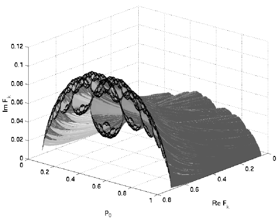
FIG. 3.: Three-dimensional representation of the cumulative functions of the reactive eigenmodes of the triadic multibaker; $({\rm Re}F_{k},{\rm Im}F_{k})$ are represented in the complex plane as a function of the probability of reaction $p_{0}$, in the case $L=1$, $k=0.1$.

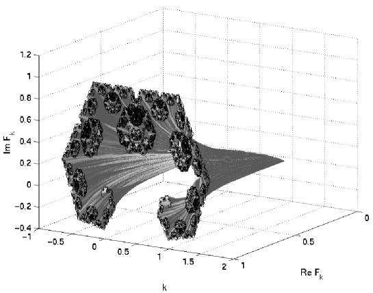
FIG. 4.: Three-dimensional representation of the cumulative functions of the reactive eigenmodes of the triadic multibaker; $({\rm Re}F_{k},{\rm Im}F_{k})$ are represented in the complex plane as a function of the wavenumber $k$, in the case $L=1$, $p_{0}=0.3$.

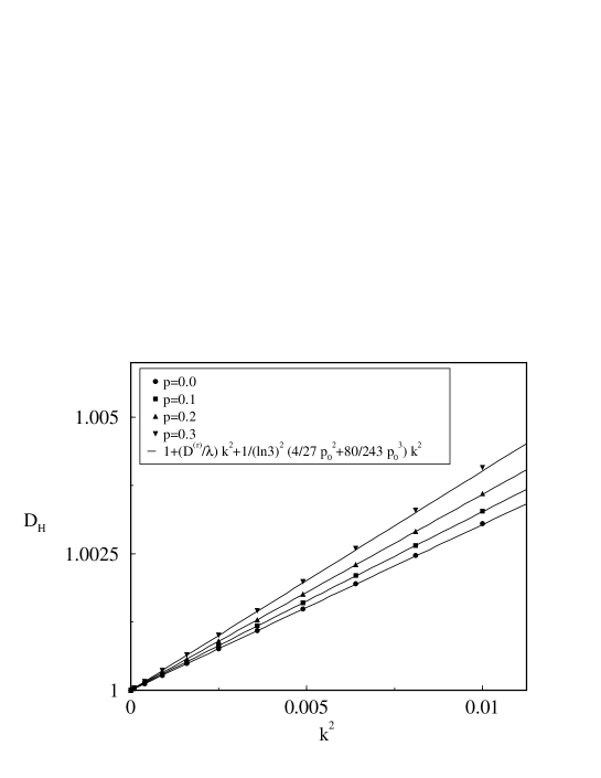
FIG. 5.: Reactive triadic multibaker: dependence of the Hausdorff dimension $D_{\rm H}$ of the cumulative functions of the reactive eigenmodes on the square of the wavenumber $k^{2}$, for $L=1$ and for different values of the reaction probability $p_{0}$. The symbols are obtained by numerical resolution of Eq. (123) and the solid line is the analytic solution (125) obtained in the limit $p_{0}\ll 1$.

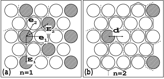
FIG. 6.: Two-dimensional reactive periodic Lorentz gas. Elementary cell of the superlattice of the catalysts (a) in the case $n=1$; (b) in the case $n=2$.

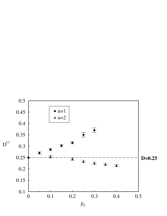
FIG. 7.: 2D reactive periodic Lorentz gas. Dependence of the reactive diffusion coefficient ${\cal D}^{\rm(r)}$ on $p_{0}$, in the case $d=2.3$, for $n=1$ and $n=2$. The value of the diffusion coefficient for $d=2.3$ is indicated for comparison.

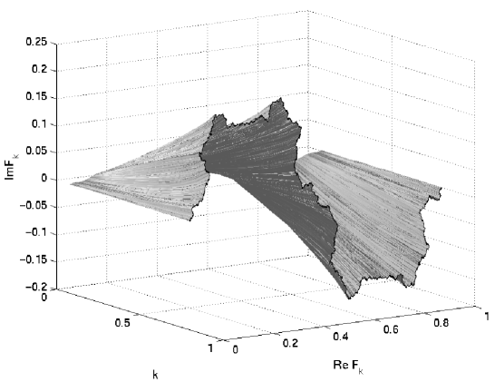
FIG. 8.: 2D reactive periodic Lorentz gas. Three-dimensional representation of the cumulative functions of the reactive eigenmodes; $({\rm Re}F_{k},{\rm Im}F_{k})$ are represented in the complex plane as a function of the wavenumber $k$, in the case $n=1$, $d=2.3$ and $p_{0}=0.3$.

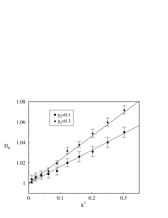
FIG. 9.: 2D reactive periodic Lorentz gas. Dependence of the Hausdorff dimension $D_{\rm H}$ of the cumulative functions of the reactive eigenmodes on the square of the wavenumber $k^{2}$, for $n=1$, $d=2.3$, $p_{0}=0.1$ and $p_{0}=0.3$. The symbols are obtained by a box-counting algorithm and the solid lines are given by Eq. (80) taking into account the corrections up to the second order in $p_{0}$.

REFERENCES

- [1] T. Gilbert, J. R. Dorfman and P. Gaspard, Phys. Rev. Lett. 85, 1606 (2000).
- [2] P. Gaspard, J. Stat. Phys. 88, 1215 (1997).
- [3] T. Gilbert, J. R. Dorfman and P. Gaspard, Nonlinearity 14, 339 (2001).
- [4] P. Gaspard, I. Claus, T. Gilbert and J. R. Dorfman, Phys. Rev. Lett. 86, 1506 (2001).
- [5] P. Gaspard and G. Nicolis, Phys. Rev. Lett. 65, 1693 (1990).
- [6] P. Gaspard and F. Baras, Phys. Rev. E 51, 5332 (1995)
- [7] J. R. Dorfman and P. Gaspard, Phys. Rev. E 51, 28 (1995).
- [8] P. Gaspard and J. R. Dorfman, Phys. Rev. E 52, 3525 (1995).
- [9] I. Claus and P. Gaspard, Phys. Rev. E 63, 036227 (2001).
- [10] B. Moran and W. Hoover, J. Stat. Phys. 48, 709 (1987).
- [11] D. J. Evans, E. G. D. Cohen and G. Morriss, Phys. Rev. A 42, 5990 (1990).
- [12] N. I. Chernov, G. L. Eyink, J. L. Lebowitz, and Ya G. Sinai, Phys. Rev. Lett. 70, 2209 (1993).
- [13] G. Nicolis and I. Prigogine, Self-Organization in Nonequilibrium Systems (Wiley, New York, 1977).
- [14] G. Nicolis, Introduction to Nonlinear Science (Cambridge University Press, Cambridge UK, 1995).
- [15] J.-P. Eckmann and D. Ruelle, Rev. Mod. Phys. 57, 617 (1985).
- [16] P. Gaspard and X.-J. Wang, Phys. Rep. 235, 291 (1993).
- [17] P. Gaspard, Chaos, Scattering, and Statistical Mechanics(Cambridge University Press, Cambridge UK, 1998).
- [18] F. Barra and P. Gaspard, Phys. Rev. E 63, 066215 (2001).
- [19] L. Van Hove, Phys. Rev. 95, 249 (1954).
- [20] J.-P. Boon and S. Yip, Molecular Hydrodynamics (Dover, New York,1980).
- [21] Ya. G. Sinai, Russian Math. Surveys 27, 21 (1972).
- [22] R. Bowen and D. Ruelle, Invent. Math. 29, 1181 (1975).
- [23] D. Ruelle, Thermodynamic Formalism (Addison-Wesley, Reading MA,1978).
- [24] P. Gaspard, Phys. Rev. E 53, 4379 (1996).
- [25] P. Gaspard and R. Klages, Chaos 8, 409 (1998).
- [26] I. Claus and P. Gaspard, J. Stat. Phys. 101, 161 (2000).