Continuum limit of amorphous elastic bodies:
A finite-size study of low frequency harmonic vibrations

Abstract

The approach of the elastic continuum limit in small amorphous bodies formed by weakly polydisperse Lennard-Jones beads is investigated in a systematic finite-size study. We show that classical continuum elasticity breaks down when the wavelength of the sollicitation is smaller than a characteristic length of approximately 30 molecular sizes. Due to this surprisingly large effect ensembles containing up to $N=40,000$ particles have been required in two dimensions to yield a convincing match with the classical continuum predictions for the eigenfrequency spectrum of disk-shaped aggregates and periodic bulk systems. The existence of an effective length scale $\xi$ is confirmed by the analysis of the (non-gaussian) noisy part of the low frequency vibrational eigenmodes. Moreover, we relate it to the non-affine part of the displacement fields under imposed elongation and shear. Similar correlations (vortices) are indeed observed on distances up to $\xi\approx 30$ particle sizes.

Pacs: 72.80.Ng, 65.60.+a, 61.46.+w

I Introduction.

Determining the vibration frequencies and the associated displacement fields of solid bodies with various shapes is a well studied area of continuum mechanics [1, 2, 3] with applications in fields as different as planetary science and nuclear physics. The increasing development of materials containing nanometric size structures leads one to question the limits of applicability of classical continuum elasticity theory, which is in principle valid only on length scales much larger than the interatomic distances [3, 4]. This question is relevant from an experimental viewpoint, since mechanical properties are inferred from spectroscopic measurements systematically interpreted within the framework of continuum elasticity [5, 6, 7, 8]. As increasingly smaller length scales are now investigated [8], direct verification of this assumption is highly warranted.

For macroscopic systems, on the other side, it is well known that the vibrational density of states in amorphous glassy materials deviates from the classical spectrum at the so called ” Boson peak“ frequency which is in the Terahertz range [9, 10, 11, 12]. The nature of the ”Boson peak“ is highly controversial [14, 15]. However, this experimental fact suggests that continuum theory is inappropriate at small length scales where the disorder of the amorphous system may become relevant [13]. Obviously, one may ask if there is a finite length scale below which the classical mechanical approach becomes inappropriate, and what the microscopic features are which determine it [4, 14, 15, 16]. Elaborating further the brief presentation given in [13], we show by means of a simple generic simulation model that, indeed, a relatively large characteristic length exists, and, second, that it envolves collective particle rearrangements.

The above questions are more generally related to the propagation of waves in disordered materials [17], and concerns foam [25] and emulsions [24] as well as granular materials [18, 19, 20], when they are submitted to small amplitude vibrations. As for these systems of current interest, the existence of an elastic limit is still a matter of debate [22], we believe that the detailed characterization of strongly heterogeneous elastic benchmark systems with a well defined continuum limit approach is crucial.

In this paper, we investigate the existence of a continuum limit in the vibrational modes of two-dimensional amorphous nanometric Lennard-Jones materials. The objects we consider are either disk-shaped clusters of diameter $2R$, as the one shown on the left side of Fig. 1, or bulk like systems without surfaces contained in a square of side $L$ with periodic boundary conditions (Fig. 1(b)). Technically, the systems are formed by carefully quenching a slightly polydisperse liquid of spherical particles interacting via simple Lennard-Jones (LJ) pair potentials into the nearest energy minimum. Due to the polydispersity the resulting structures are isotropic and amorphous, i.e. exhibit no long range crystalline order. The force network (Fig. 1) appears to be strongly varying with weak and tensile zones (red) embedded within a rigid repulsive skeleton (black). These ”force chains“ are very similar to those found in cohesionless granular media without attractive forces [21]. This feature may be added to the list of similarities which have been noticed between granular and amorphous (glassy) materials [22, 23, 24]. As the force network is strongly inhomogeneous, the relevance of the quenched stresses is a natural question [4].

We investigate the vibrational modes of these objects using atomic level simulations. All particle coordinates and interparticle forces are exactly known here, and it is possible to calculate the vibration frequencies around an equilibrium position, by exact diagonalization of the so called dynamical matrix [27] expressible in terms of the first and second derivatives of the interparticle interaction potentials. We have carried out a systematic comparison of these eigenfrequencies $\omega(p)$ ($p$ being an index increasing with frequency) obtained numerically with those predicted by continuum elasticity for two dimensional objects of increasingly large sizes [1]. We concentrate on the lowest end of the vibrational spectrum, since this is the part that corresponds to the largest wavelengths for the vibrations, and should reach first the continuum limit. These frequencies are also those which are probed in low frequency Raman scattering experiments [8], in order to determine the typical size of nanoparticles.

The key result of this paper is to show the existence of a characteristic wavelength (thus a characteristic size) beyond which the classical continuum limit is valid, but below which it is erroneous. Moreover, we show the existence of rotational structures (vortices) of similar sizes, when the system is submitted to simple mechanical sollicitations (traction and shear). The size of these vortices is relatively large ($\approx 30$ average interatomic distances). We discuss the relation between the sizes of the vortices and the limit of applicability of the classical continuum theory by computing the elastic moduli, by studying the symmetry of the nanoscale stress tensor, and by identifying the low frequency vibrational eigenmodes.

Our paper is arranged as follows: In Sec. II we summarize some basic relations and results of classical continuum theory for two dimensional elastic bodies. Simulation techniques, sample parameters and preparation protocols of our model amorphous systems are explained in Sec. III and simple system properties are discussed. In Sec. IV we analyse histograms and spatial correlations of the quenched forces and of the stiffness of the bonds. A weak enhancement of the rigid skeleton is demonstrated for small systems. The next two sections contain the key results of this paper. In Sec. V we discuss the mechanical properties of a periodic bulk system under elongation and shear, we compute the elastic moduli and we characterize the non-affine displacement field generated. The eigenvalues and eigenvectors and their departures from the continuum prediction are analyzed in Sec. VI. We conclude with a summary of our results in Sec. VII.

II Theory

Before presenting our computational results we give here a short synopsis of assumptions and results of classical continuum elasticity in two dimensions, relevant for the subsequent discussion of our numerical results.

A Continuum description of an isotropic elastic body in 2D.

The main assumption of classical elasticity [28], is that the system can be entirely described by a unique vectorial field: the displacement field $\mbox{$\underline{u}$}(\mbox{$\underline{r}$})$, describing the displacement of a volume element from its equilibrium position $\underline{r}$. As we are interested in systems at zero temperature, energy and free energy are obviously identical. The Landau expansion[2] of the energy $\delta E$ per unit volume is expressed in terms of $\underline{u}$ and its first derivatives. Due to translational and rotational invariance [28] of $\delta E$, it depends only up to second order on the symmetric part of $\mathrm{\mathbf{grad}}\,\,\mbox{$\underline{u}$}$, the (linearized) strain tensor $\epsilon_{\alpha\beta}\equiv 1/2~{}(\partial u_{\alpha}/\partial x_{\beta}+\partial u_{\beta}/\partial x_{\alpha})$ with $x_{1}=x$ and $x_{2}=y$ for the coordinates. Moreover in linear elasticity (that is in the lowest order in the Landau expansion), for isotropic and homogeneous systems only two Landau parameters are required, thus:

$$\delta E=\frac{\lambda}{2}\left(\epsilon_{xx}+\epsilon_{yy}\right)^{2}+\mu\left(\epsilon_{xx}^{2}+\epsilon_{yy}^{2}+2\epsilon_{xy}^{2}\right)$$ (1)

where we have defined the two phenomenological Lam coefficients $\lambda$ and $\mu$. $\mu$ is the so called shear modulus, and $\lambda$ takes part in the compressibility $k=\lambda+\mu$. Below, we will discuss two methods to determine them in a computer experiment. The stress tensor can be defined as the conjugate variable of the strain tensor,

$$\sigma_{\alpha\beta}\equiv\partial\delta E/\partial\epsilon_{\alpha\beta}.$$ (2)

In this definition $\sigma_{\alpha\beta}$ it obviously a symmetric tensor. We will see later that a microscopically constructed stress tensor can, however, violate this symmetry condition at small length scales (section  II C).

For the remaining three independent stress tensor elements, one gets from Eqns (1) and ( 2) the standard Hooke ’s relations:

$$\sigma_{xx} = (\lambda+2\mu)\epsilon_{xx}+\lambda\epsilon_{yy}$$ (3)

$$\sigma_{yy} = (\lambda+2\mu)\epsilon_{yy}+\lambda\epsilon_{xx}$$ (4)

$$\sigma_{xy} = \sigma_{yx}=2\mu\epsilon_{xy}.$$ (5)

We use these formulae in Sec. V to measure directly the Lamé coefficients from the forces generated in a periodic box under external strain. It is easy to work out from Eq. ( 3) that in 2 dimensions the Poisson ratio is given by $\nu=\lambda/(\lambda+2\mu)$ with an upper bound $1$ (and not $1/2$ as in 3D) [2].

As it is well known[1, 2], the equations of motion $\rho\partial\sigma_{\alpha\beta}/\partial x_{\alpha}=\ddot{u}_{\alpha}$ together with the constitute Eqns. ( 3) correspond to wave equations with boundary conditions depending on the problem of interest: for the periodic box problem the solutions must have the same periodicity, and the freely floating disk-shaped aggregate requires vanishing lateral and radial stresses on its surface. The velocities of transverse and longitudinal waves which solve these wave equations are given in terms of the Lamé coefficients, i.e. one has $c_{T}^{2}=\mu/\rho$ and $c_{L}^{2}=(\lambda+2\mu)/\rho$ where $\rho$ is the particle density [1]. We remind that $c_{L}>c_{T}$ and that transverse modes thus correspond generally to smaller eigenfrequencies.

The solutions for the periodic box case are of course the plane waves with a wavevector quantified by the boundary conditions, $(k_{x},k_{y})=\frac{2\pi}{L}(n,m)$, with wavelength [29]

$$\lambda(p)=\lambda(n,m)=\frac{2\pi}{||\mbox{$\underline{k}$}||}=\frac{L}{(n^{2}+m^{2})^{1/2}}$$ (6)

and with dimensionless frequency

$$\Omega^{2}_{T,L}(p)\equiv\left(\frac{\omega(p)L}{2\pi c_{T,L}}\right)^{2}=n^{2}+m^{2}$$ (7)

with two quantum numbers $n,m=0,1,...$. The running index $p$ increases with frequency. In the continuous case, the dispersion relation is linear, and the frequency is straightforward. Hence, eigenfrequencies are characterized by a pair of different integers. They are eight-fold degenerated if $n\neq m\neq 0$ and four-fold in all other cases. The associated plane waves travel in two opposite and orthogonal directions.

The situation for disk-shaped objects is somewhat more complex [1], with again two quantum numbers $n$ and $k$ characterizing the eigenmodes. The quantum number $k$ is associated with the angular dependency of the displacement field (and is due to the $2\pi$ periodicity), and the number $n$ to its radial dependency. The eigenfrequencies are obtained by solving the non linear dispersion relation. They are of the form

$$\Omega^{2}_{T,L}(p)\equiv\left(\frac{\omega(p)2R}{2\pi c_{T,L}}\right)^{2}=f_{nk}(\nu)$$ (8)

where $\nu$ is the Poisson ratio given above. The eigenvectors are related to Bessel functions [1] which may be approximated locally by plane waves if $\lambda(p)\ll R$. Vibrational modes of disks are either non degenerate (for axially symmetric modes) or have two-fold degeneracy (for all other modes). Indeed, for $k>0$, for every solution whose amplitude is $\propto e^{ik\theta}$, one finds a second solution, orthogonal to the first one, with amplitude $\propto e^{ik(\theta+\Delta\theta)}$ where $\Delta\theta=\pi/2k$. Every additional solution with the same $k$ is a linear combination of these two vectors. For axially symmetric modes ($k=0$), the above argument does not apply; any additional solution found by turning the coordinate system is identical to the first one.

We finally stress the obvious: degenerate eigenvalues are inherent to the continuum treatment of highly symmetric systems. The failure to observe them indicates either the lifting of the relevant symmetry or the breakdown of continuum theory.

B Pair potential systems with central forces.

In a simulation one has the advantage to know all the individual contributions to the total energy. The situation is particularly simple if one has to deal with interparticle pair potentials $U(r_{ij})$ ($r_{ij}$ being the interparticle distance) such as the LJ potential we use, and if we stay at zero temperature. In this case, the difference of the total potential energy

$$E_{p}=\sum_{i=1}^{N-1}\sum_{j>i}^{N}U(r_{ij})$$ (9)

due to a displacement field $\underline{u}$ can be written to second order as a Hessian form $\delta E_{p}=\frac{1}{2}\mbox{$\underline{u}$}^{t}\cdot\mbox{$\underline{\underline{M}}$}\cdot\mbox{$\underline{u}$}$ in terms of the $(2N)\times(2N)$ dynamical matrix $\underline{\underline{M}}$ whose elements are given by

$$-r_{ij}^{2}M_{i\alpha,j\beta}=r_{ij}t_{ij}\left(\delta_{\alpha\beta}-n_{\alpha}n_{\beta}\right)+r_{ij}^{2}c_{ij}n_{\alpha}n_{\beta}$$ (10)

$\underline{n}$ being the unit vector of the bond (for simplicity, we do not indicate the dependence of $\underline{n}$ on the particle indices $i$ and $j$), $t_{ij}\equiv\partial U(r_{ij})/\partial r_{ij}$ the tension and $c_{ij}\equiv\partial^{2}U(r_{ij})/\partial r_{ij}^{2}$ the stiffness of the bond between two interacting beads $i$ and $j$. The first one is related to the stresses “quenched” in the bulk, but as we will see later it is in general small in comparison with the second one. As in the present study the mass $m$ of each monomer is set equal to unity (even though the particle diameters are polydisperse) the Euler-Lagrange equation $\mbox{$\underline{\underline{M}}$}\cdot\mbox{$\underline{u}$}+m\ddot{\mbox{$\underline{u}$}}=0$ is solved directly by eigenfrequencies and displacement fields obtained simply by diagonalisation of the dynamical matrix.

Assuming constant deformations (purely affine displacement field) under elongation and shear, one may use the dynamical matrix to calculate the Lamé coefficients. Comparing [30] the Landau expression Eq. ( 1) and the microscopic energy information in Eq. ( 9), we get

$$\lambda_{a} = \frac{1}{A}\sum_{ij}\left[r_{ij}t_{ij}n_{x}^{2}n_{y}^{2}+r_{ij}^{2}c_{ij}\right((n_{x}^{4}+n_{y}^{4})/2-2n_{x}^{2}n_{y}^{2}\left)\right]$$ (11)

$$\mu_{a} = \frac{1}{A}\sum_{ij}r_{ij}^{2}c_{ij}n_{x}^{2}n_{y}^{2}$$ (12)

with $A$ being the total surface. The sums run over all pairs of particles. As an affine displacement field is assumed to be valid down to atomic distances the coefficients have been assigned an index $a$ to distinguish them from the true macroscopic Lamé coefficients that will be calculated later. It is instructive to consider the simple one dimensional analogy, i.e. a long string of connected springs with force constants $c_{l}$, to appreciate the approximation made in the above equations. We recall that the effective macroscopic Young modulus is $\lambda=1/\langle 1/c_{l}\rangle$ rather than $\lambda_{a}=\langle c_{l}\rangle$. This is due to the fact that the tension along the chain is constant but not the displacement field. Hence, Eqns. ( 12) are in general only good approximations if the dispersion of the effective spring constants is small and an external macroscopic strain is locally transmitted in an affine way. ($\lambda$ is then indeed given by the mean coupling constant with a negative quadratic dispersion correction in leading order.) We will test this assumption in Sec. V and estimate the length below which the affinity approximation becomes problematic.

C Definition and Measurement of stress tensor.

In the elastic continuum theory (section II A), the stress tensor is usually introduced by considering the forces per unit length exerted between adjacent volume elements. The total energy $\delta E$ thus corresponds to the work of internal forces. At a microscopic level, a natural way of extending this macroscopic approach is to compute $\sigma_{\alpha\beta}$ as the sum of forces per unit length $(-t_{ij}n_{\alpha}/b)$ exerted in the $\alpha$ direction through the side perpendicular to the $\beta$ direction of a small volume element of size $b$. A stress tensor defined in this way can be asymmetric. The usual, macroscopic proof [2, 3] of the symmetry of $\sigma$ is based on the fact that intermolecular forces are short-ranged. Hence, one expects symmetry of the microscopic stress tensor (obtained from the ’macroscopic’ definition) only for volume elements of size $b$ much larger than the range of intermolecular forces. In section  V, we will investigate how this macroscopic limit is reached.

Note that our definition of the stress tensor, does not correspond strictly to the usual [4, 31] microscopic Kirkwood definition

$$\sigma_{\alpha\beta}(i)\equiv-\Sigma_{j}t_{ij}n_{\alpha}.n_{\beta}$$ (13)

which is necessarily symmetric. Although both quantities yield the same macroscopic stress tensor, the definition we are using is more appropriate to illustrate deviations from macroscopic behavior at small scales. Another method for illustrating these deviations can be found in Ref. [31]. In this work, the local breakdown of rotational invariance in a disordered system was shown to imply contribution of the asymmetric part of $\underline{u}$ to the local elastic energy. Defining $\sigma_{\alpha\beta}$ as $\partial\delta E/\partial(\partial u_{\alpha}/\partial\beta)$ in place of Eq. ( 2), it can be shown that the contribution of the asymmetric part of $\sigma$ to the local energy is related to the work of the fluctuating part of the forces on the fluctuating part of $\underline{u}$. In reference  [31], it was shown that this contribution vanishes only for very large systems.

III Sample preparation and characterization.

Systems with two different boundary conditions (disks and periodic bulk systems) and three quench protocols have been simulated. In this section we discuss some technical points concerning the simulation methods and the sample preparation protocols and parameters. The details of the protocols and some properties of the final configurations are summarized in the Tables I, II and  III.

In the present study we use a shifted LJ potential [32] for polydisperse particles with $U_{LJ}(r)=\epsilon\left((r_{0}/r)^{12}-2(r_{0}/r)^{6}\right)+const$ for $r<2r_{0}$ and $U_{LJ}(r)=0$ otherwise, correctly regularized. We have written the potential in terms of the distance $r_{0}\equiv(a_{i}+a_{j})/2^{5/6}$ where the LJ force vanishes. Natural LJ units are used, i.e. we set the energy parameter $\epsilon\equiv 1$, the particle mass $m\equiv 1$ and the mean diameter $a=\langle a_{i}\rangle=1$. Note that while the particle mass is strictly monodisperse the particle diameters $a_{i}$ are homogeneously distributed between $0.8$ and $1.2$. This corresponds to a polydispersity index $\delta a/a\approx 0.12$ which is sufficient to prevent large scale crystalline order. We did not attempt to make the particles even more polydisperse fearing demixing or systematic radial variation of particle sizes in the case of disk-shaped aggregates.

The quench generally starts with molecular dynamics (MD) at some fixed temperature using a simple velocity rescaling thermostat [32]. As integrator we use the velocity Verlet algorithm [33] with a time increment $\delta t=0.001$. The temperature remains constant over a fixed time interval of $1000$ MD steps for each temperature step. This was sufficient to relax systems into a steady-state (obviously, not necessarily the equilibrium) as monitored by pressure and system energy. Unfortunately, no more detailed characterization of the ageing as a function of the quench rate has been recorded. Following the initial MD sequence we quench the systems further down using a steepest descent (SD) method with a frictional force proportional to the total particle velocity and an additional damping term proportional to the relative velocity of interacting particles. We use a small value of order one for both friction constants and a simple leap-frog like integrator consistent with the velocity depended force [33]. The particle motion is overdamped. The systems were cooled down with SD over a period of at least $1000$ time steps. Finally, the conjugate gradient method (CG) [33, 34] was iterated till the configurations reach their local energy minima. Double precision was used at every stage.

An example for a disk-shaped aggregate has already been presented in fig. 1(a). Two different protocols have been employed to generate such disks:

• Protocol I: The starting point of the first protocol is a not too dense LJ liquid droplet of radius $R_{i}$ and $\rho_{i}\approx 0.9$ and temperature $T_{i}=0.1$. The initial radius $R_{i}$ is chosen such that the final mean radius $R$ becomes not too different. We cool the systems with MD steps at $T=0.1,0.05,0.01,0.005$ and $0.001$. As described above, we finally quench each system into its local minimum using a sequence of SD and CG steps. See Table I for details.

• Protocol II: In the second case spherical disks of radius $R_{i}$ were cut out of amorphous periodic systems already prepared at $T=0$ (see Protocol III) and $\rho=0.925$ and the disks are quenched as before with SD and CG. No finite temperature MD step was included here. See Table II for details. The second protocol is much faster than the first one which might, however, mimic better the actually occurring aggregation process in real systems.

The radius $R=\sqrt{2(I_{1}+I_{2})/N}$ of quenched cluster is obtained from the eigenvalues $I_{1}>I_{2}$ of the inertia tensor of the cluster. The mean density $\rho=<N/\pi R^{2}>$ obtained accordingly is a weakly decreasing function of the particle number as can be seen from the Tables I and II. This is expected and in qualitative agreement with the decreasing Laplace pressure $P\propto 1/R$. Note that the pressure is very small for all the disks (Protocol I and II alike) and is not indicated. We have also tried to characterize the shape of the disks and have indicated the excentricity $e=\sqrt{1-I_{2}/I_{1}}$. As can be seen, small aggregates are strongly elliptic, but the effect is much stronger for the first slow aggregation protocol. This is probably due to capillary waves formed at $T=0.1$ which are subsequently frozen in. Obviously, ellipticity is one possible cause for lifting of the eigenfrequency degeneracy. This effect should, however, become small for larger clusters where $e$ vanishes (Tab. I and II). Moreover, we will see later that the mechanical properties of our aggregates do not depend significantly on the quench protocol.

Periodic bulk systems, such as the one presented in Fig. 1(b), have been prepared following the third protocol and are summarized in Table III. We started here with equilibrated liquids at $T=1$ which were then subsequently cooled down with temperature steps at $T=0.5,0.1,0.05,0.01,0.005$ and $0.001$. Systems between $L=7a$ and $L=208a$ and containing from $N=50$ up to $N=40,000$ particles have been sampled.

For $N=10,000$ particles we have systematically scanned over density varying the box size from $L=100$ to $L=110$. This was done in order to find — for the given protocol — a working point density for which large bulk systems correspond to a near zero pressure state $P(T=0)\approx 0$, thus the mechanical properties of the bulk systems correspond to the free-floating aggregates. Note that only one configuration has been sampled for this measurement sequence. As a sideline, we draw attention to the fact that systems with $P<0$ while mechanically stable in a periodic box are thermodynamically unstable at low temperature. If more time would be given to the systems to equilibrate as allowed by the protocol phase separation would occur. Indeed we find evidence for the formation of small holes for $\rho<0.85$. In all other cases we find that density is perfectly homogeneous down to a scale typical of the interatomic distance and density fluctuations are easily excluded as a microscopic candidate for explaining the slow continuum approach. Our systematic finite-size study, i.e. the variation of box sizes $L$, was performed at fixed density $\rho=0.925$. In order to scale correctly the eigenfrequencies of the aggregates we have also recorded the Lamé coefficients as a function of density. We have checked that the particle energies $E$, Lamé factors $\lambda_{a}$ and $\mu_{a}$, mean effective spring constants $\langle r_{ij}^{2}c_{ij}\rangle$ (which are included in the different tables) do not depend significantly on the different symmetries and quench protocols, for a given density. It is reassuring that all the results we obtained are robust with regard to the variation of the quench protocol even though history dependence must obviously play a role for the details. Typically, we have generated $20$ configurations for each $L$ and in terms of CPU hours this was the most demanding part of this study. The simulations have been performed on a local workstation cluster over a period of one year.

Interestingly, we notice in Table III that the pressure, the particle energy and the Lamé coefficient $\lambda$ increase systematically in small boxes. This is shown specifically for $\lambda$ in Fig. 4(b). These finite-size effects indicate correlations on a similar length even in larger systems. We will now turn to the characterization of these correlations, by first studying the dynamical matrix, and the quenched stresses.

IV Contributions to the dynamical matrix: Quenched forces and spring constants

In this section we discuss various distributions and correlation functions associated with the quenched particle positions, forces and spring constants which contribute to the dynamical matrix (Eq. ( 10)). We attempt a characterization of the frozen in disorder visualized in Fig. 1 where the snapshots reveal strong spatially correlated fluctuations. Specifically, we ask if it is possible to extract a characteristic length scale solely from the distribution of weak and rigid regions which might be a candidate to explain the large crossover length scale $\xi$ mentioned in the Introduction. We start by giving some additional information concerning the snapshots, turn then to the histograms and discuss finally the fractal structure of the quenched forces.

A timely justification for discussing quenched forces lies in the current interest of their role in granular materials, foams and glassy colloidal systems [4, 21, 22, 23, 24, 25, 26]. It has been suggested by S. Alexander[4] and others that the quenched forces might contribute to the unusual mechanical and rheological properties in these systems. However, to put this immediately into perspective, quenched forces are unlikely candidates to rationalize alone the slow continuum approach discussed in Sec. VI, basically, since their average contribution to the dynamical matrix is weak: $\langle r_{ij}^{2}c_{ij}\rangle\gg\langle r_{ij}t_{ij}\rangle$. This inequality is revealed in Table III. We come back to this in Sec. VI where we discuss the contribution of the quenched forces to the eigenmodes.

The second and more important point we want to make here is that for a given potential the first and the second derivative contain essentially the same information. Both together are expressions of the same disorder generated by the complex cooling procedure — which is subject to the one chosen potential and its derivatives. It is the final positional disorder which matters, not the individual contributions to the dynamical matrix. If the width of the lines between the particle positions shown in the snapshots (Fig. 1) has been chosen proportional to the interaction force rather than the spring constant this was done mainly for artistic reasons. Resembling snapshots can be obtained, using as a scale for the line width either the spring constants or the trace $m_{ij}=M_{ix,jx}+M_{iy,jy}$ of the dynamical submatrices. Such pictures are direct visualizations of the dynamical matrix.

The snapshots Fig. 1 reveal that the structure of the force network is very inhomogeneous, but isotropic on larger scale. They show also evidently that the quenched disorder is not much affected by the different symmetries (circle or square) and quench protocols. This corroborates the robustness of the system properties with regard to the chosen protocol mentioned in the previous section. This is also supported by the different histograms regrouped in Fig. 3.

Systems of the three protocols are included in first of both graphs Fig. 3(a) where we discuss the distribution of distances of interacting particles (inset) $r_{ij}/r_{0}$ and of the tensile forces $t_{ij}$ (main figure) for relatively large systems containing $N=10,000$ particles. Comparison shows that there is essentially no dependence on quench protocol. Note that this is only a technical point and will make life easier when we analyse the eigenvalue spectrum of disk-shaped aggregates. The peak at $r_{ij}=r_{0}$ in the inset corresponds to the peak for $t_{ij}=0$ in the main figure of Fig. 3(a). Hence, most of the interactions have achieved to minimize their energy although this is not required for global mechanical stability. The distribution of the repulsive forces (negative tensions) is Gaussian. Incidentally, this is quite different from the recently reported exponential force distributions in granular matter [21, 23]. Interestingly however, the tail of the force distribution becomes more and more exponential upon decreasing of the system size. We do not show this here, as the same effect is presented in the second panel (Fig. 3(b)) for the trace of the dynamical submatrices. Various system sizes as indicated in the figure are given here for the third protocol at $\rho=0.925$. This demonstrates that the tail of distribution which corresponds to very rigid contacts becomes enhanced due to finite-size effect for systems below $L\approx 20a$. A very similar figure could also be given for the distribution of spring constants. Note that the peak on the left side of Fig. 3(b) is due to the slow variation of the spring constant for large distances and corresponds to distances seen in the shoulder on the right of the histogram in the inset.

In fig. 2 we show two of several attempts to analyse the correlations and fractal structure of force chains (or the spring constants) in view of extracting a characteristic size. We focus on strong repulsive forces and strong positive spring constants. Only results from the first measurements are reported as both yield similar results. In a first step we obtain the network of all interactions with (negative) repulsive tensions above some threshold $t_{u}$ and compute then on these sets various correlation functions. The functions $\langle\cos^{2}(\tau)\rangle$ traced in Fig. 2(a) attempt to put the visual impression of linear force chains in quantitative terms. Here $\tau$ denotes either the angle between the directors $n_{i}$ and $n_{j}$ of the links $i$ and $j$ (spheres) or the angle between the director $n_{i}$ of link $i$ and the direction $n_{ij}$ between the links $i$ and $j$ (squares). The difference between both methods is small. The correlation dies out only after about six oscillations. No significant difference have been found by increasing or decreasing the threshold $t_{u}$. The decay of the envelope is exponential with a length scale of the order of the mean bead size. Hence, while rigid regions seems to be spatially correlated, this does not, apparently, introduce a new length scale. Note that the situation is similar in granular materials [20].

The second part of Fig. 2 shows a direct attempt to elucidate the fractal structure of the network of quenched forces by means of the standard box counting technique. Here we count the number of square boxes of linear size $b$ needed to cover all the links between beads carrying a repulsive force smaller than $t_{u}$. For small $b$ where every box contains only one link the differential fractal dimension is zero. In the opposite limit where the boxes are much larger than the average distance between links, the differential fractal dimension must equal the spatial dimension, i.e. $d_{f}=2$. The power law slope $d_{f}=1$ in between both limits indicates the typical distance where the contact network with $t_{ij}<t_{u}$ has a linear chain like structure. For example, we find a tangent with slope $d_{f}=1$ at $b\approx 6a$ for $t_{u}=-5$. This distance is strongly increasing if we focus on more and more rigid subnetworks (decreasing $t_{u}$). Note, however, that there is no finite $b$-window with $d_{f}=1$ and in a strict sense there is again no characteristic length scale associated with linear structures. A simple visual inspection of Fig. 1 that would suggest a characteristic length scale of the repulsive force network much larger than the interatomic separation is apparently incorrect and possibly caused by the natural tendency of our brains to emphasize linear patterns [35].

As a simple benchmark for the spatial correlation of the force network, we have distributed links randomly. The box counting of these uncorrelated links gives the dashed lines. Unfortunately, these are virtually identical to the fractal dimension characterization of the force chains in the LJ systems and it is a very tiny difference (at least in this characterization) which is related to the spatial correlations. Obviously, this does not mean the forces are uniformly distributed as clearly shown by the snapshots and by the large number of oscillations in the correlation function.

In summary, we provide evidence for a strong dispersion in the dynamical matrix, i.e. in the local elastic properties of our systems. Although linear chain like structures exist apparently, this does not give rise to an additional characteristic length — defined as the screening length in an exponential decay — much larger than the mean particle distance.

V Elongation and Shear: Elastic moduli and non-affine displacement field

A direct way of illustrating the failure of classical elasticity at small scales is to investigate the displacement field in a large, deformed sample. If the system is uniformly strained at large scales, e.g. by compressing or shearing a rectangular simulation box, classical elasticity implies that the strain is uniform at all scales, so that the atomic displacement field should be affine with respect to the macroscopic box deformation. If this is true Eqns. ( 12) should provide reliable estimates of the Lamé coefficients. Since the latter can be independently measured in a computer experiment from the generated stress differencies using Hooke’s law (Eqns. ( 3)) this provides a direct and crucial test for the affinity assumption.

Our numerical test proceeds in three steps:

• Each initial configuration is given a first quick CG quench with quadruple precision to have a more precise estimate for the unstrained reference system. This is necessary since the stress differences we compute are very small for strains in the linear response regime and the numerical accuracy of double precision simulation runs turns out to be insufficient.

• Second, we perform an affine strain of order $\epsilon$ of both the box shape and the particle coordinates. We consider both an elongation in $x$-direction ($L_{x}\rightarrow L_{x}(1+\epsilon)$,$r_{x}\rightarrow r_{x}(1+\epsilon)$) and a pure shear using Lees-Edwards boundary conditions [32] together with $r_{x}\rightarrow r_{x}+r_{y}\epsilon$. (We refer here to the principal box particle coordinates $(r_{x},r_{y})$ of the periodic configurations.)

• Finally, we quench with CG the configurations into the local minima while maintaining the strain at the boundaries. For given boundary conditions in the linear regime the solution must be unique.

The differences of particle positions, forces and total energies computed at each step are recorded. We stress that this procedure is technically not trivial and that great care is needed to measure physically sound properties.

We have systematically varied $\epsilon$ over several orders of magnitude from $\epsilon=1$ down to $\epsilon=10^{-9}$ (not shown). The induced displacement field is reversible linear in the amplitude of the imposed initial strain for an initial strain in a window $10^{-4}\leq\epsilon\leq 0.1$ which decreases (for unknown reasons) somewhat with system size. Obviously, for higher strains the linearity of Eq. ( 3) must eventually break down. The departure from linearity below the given strain window is due to numerical accuracy.

Using Eq. ( 3) for the stress tensor averaged on the whole system and the averaged strain field, we obtain the true macroscopic Lam coefficients $\lambda$ and $\mu$. Within the given strain window the measured $\lambda$ and $\mu$ coefficients are strain independent, thus confirming the linearity of the elastic response in this range. The values of $\mu$ and $\lambda$ are presented in Fig. 4 where we have compared them with the affine field predictions. (Note that the Poisson ratio $\nu\approx 2/3$ is larger than $1/2$ which is permissible in a 2D system as clarified in Sec. II.) The coefficients relying on a negligible non-affine field (open symbols, obtained from Eq. ( 12)) differ by a factor as large as two from the true ones. Clearly, a calculation taking into account the non-affine character of the displacements is necessary for disordered systems. Indeed, it is simple to work out from the values given in the figures that, in a simple elongation, a finite energy fraction $(\lambda_{a}+2\mu_{a})/(\lambda+2\mu)-1\approx 1/4$ of the total strain can be recovered from the non-affine displacements. In a pure shear, the energy fraction $\mu_{a}/\mu\approx 1/2$ is even larger; only the compressibility $k=\lambda+\mu$ remains unchanged. Hence, in quantitative terms the non-affinity of the atomic displacements is not a negligible effect.

The non-affine component $\delta\mbox{$\underline{u}$}$ of the atomic displacement field in large systems subject to an elongation in $x$ direction is illustrated in the snapshot Fig. 5(a). A similar snapshot holds in case of a pure shear (Fig. 5(b)). In some regions, the displacement is much larger than expected from a purely affine transformation (Note that even the non-affine part of the displacement field is strictly linear in $\epsilon$ within the strain interval indicated above). Local displacements transverse to the direction of the elongation are allowed, and organize coherently into vortices. The transversal direction thus cannot be neglected, showing that the modelling approach put forward in Ref. [18] is not realistic. The crossover length $\xi$ mentioned in the Introduction manifests itself through correlated deviations from a purely affine displacement. Visual inspection tells us that the sizes of the vortices and $\xi\approx 30a$ are comparable.

The two correlation functions presented in Fig. 6 confirm this visual impression. The first one shows the correlation function $C_{u}(r)=\langle\delta\mbox{$\underline{u}$}(r)\cdot\delta\mbox{$\underline{u}$}(0)\rangle$. The striking anti-correlation for $r\ll 30a$ is in agreement with the size of the vortices seen in the displacement fields. That the displacement field is indeed correlated over a similar size is further elucidated in Fig. 6(b). Here we consider the systematic coarse-graining of the non-affine displacement field

$$\delta\mbox{$\underline{\cal U}$}_{j}\equiv\frac{1}{N_{j}}\sum_{i\in V_{j}}\delta\mbox{$\underline{u}$}(\mbox{$\underline{r}$}_{i})$$ (14)

of all $N_{j}$ beads contained within the square volume element $V_{j}$ of linear size $b$. The mean-squared average $U_{x}(b)\equiv\langle\delta{\cal U}_{x,j}^{2}\rangle_{j}^{1/2}$ is plotted versus the size of the coarse-graining volume element $b$. We have normalized the function by its value at $b=1$. The coarse-grained field decreases very weakly for $b<30a$ and only for much larger volume elements we find the power law slope $-1$ expected for uncorrelated events. As for symmetry reasons the total or mean non-affine field vanishes we have $U_{x}(b\rightarrow L)\rightarrow 0$ for very large volume elements. Apart from this trivial system size dependence $U_{x}$ approaches a system size independent envelope for $b\ll L$, as can be clearly seen from the figure.

Barely distinguishable functions have been obtained for $U_{y}$ (not depicted) which demonstrates the isotropy of the non-affine displacement fields which may also be inferred straight from the snapshots and appropriately chosen correlations functions. Similar characterizations can be obtained from a standard Fourier transform of $\delta\mbox{$\underline{u}$}(x,y)$ and from the gradient fields defined on the coarse-grained field $\delta\mbox{$\underline{\cal U}$}_{j}$. These are again not presented.

In the rest of this section, we consider the local stresses generated by the applied macroscopic deformation. We show in Fig. 7 the variance $\langle(\sigma_{xy}-\sigma_{yx})^{2}\rangle$ averaged on various boxes of size $b$. Here, the stress tensor $\sigma_{\alpha\beta}$ has been defined, as in classical mechanics, as the average force exerted in the $\alpha$ direction through the side perpendicular to the $\beta$ direction of the volume element of size $b$. We see clearly in the Fig. 7 that for a size $b<30a$, this stress tensor is asymmetric, and that the asymmetry decreases exponentially to zero for larger sizes. In agreement with the discussion of section II, this effect must be due to the lack of invariance of the energy under translations or rotations for volume elements of sizes $<30a$.

We note that the length scales observed in all these plots are relatively large compared to the particle size, but are not in the classical sense characteristic lengths appearing in the exponential decay of a correlation function. An important consequence of the large spatial correlations is that calculations of Lamé coefficients are prone to finite-size effects for system sizes similar and below $\xi$. This explains qualitatively the peculiar system size dependence of the Lamé coefficients reported in Fig. 4(b).

VI Vibration modes

In this section we discuss finally the eigenvalues and eigenvectors of the different systems we have generated. For each configuration the lowest ($p\leq 1000$) vibration eigenfrequencies and eigenvectors have been determined using the version of the Lanczos method implemented in the PARPACK numerical package [36]. As stressed in the introduction we concentrate on the lowest end of the vibrational spectrum, since this is the part that corresponds to the largest wavelengths for the vibrations.

We continue and finish first the discussion of disk-shaped aggregates which started with the snapshot Fig. 1(a). This being done we focus more extensively on the simpler periodic glassy systems (Protocol III) and discuss subsequently their eigenfrequencies and eigenvectors. This allows us to pay attention to central questions of strongly disordered elastic materials without being sidetracked by additional physics at cluster boundaries (ellipticity, radial variation of material properties etc.).

A Eigenmodes of disk-shaped aggregates

The first non-trivial eigenvalues ($4\leq p\leq 11$) for the two protocols for disk-shaped clusters are shown in Fig. 8(a). The first three eigenmodes have vanishing eigenfrequencies because of two translational and one rotational invariance. Aggregates of different sizes are presented as indicated in the figure. The frequencies are rescaled with the disk diameter $2R$ as suggested by dimensional considerations or continuum theory. This scaling is roughly successful for all systems included. For the smaller systems (e.g., for the example with $N=732$ given) $\omega$ do not present the degeneracies of the continuum theory. If we increase the system size steps appear and the eigenfrequencies start to regroup in pairs of two following the continuum prediction. This is well verified for the largest disk we have created containing $N=32,768$ beads. The horizontal lines are comparisons with continuum theory with appropriate density and where the Lamé coefficients (and, hence, the sound velocities) have been taken accordingly from Table III. The comparison of the two protocols (I and II) for $N=4096$ shows that, perhaps surprisingly, the quench protocol does not matter much if only the clusters are large enough and the excentricity sufficiently weak. Note that this is definitely not true for small disks where the excentricity matters.

A schematic representation of the displacement fields for the lowest eigenmodes of a large disk-shaped cluster ($R=60$) is given in Fig. 10. For such large cluster the displacement fields essentially conform to standard elastic behavior. The two quantum numbers $n$ and $k$ are indicated for each mode. The snapshots demonstrate nicely the two-fold degeneracy for all the modes which are not axisymmetric (the first ten fields). We confirm that corresponding pairs are turned with respect to each other by an angle $\Delta\theta=\pi/2k$, e.g. for the first non-trivial modes $p=4$ and $p=5$ where $k=2$ by an angle $\Delta\theta=45^{0}$. The disk wobbles in these modes between two perpendicular slightly elliptic shapes. The numerics returns arbitrary linear superpositions of eigenvectors associated with the same eigenvalue. As we have at most a two-fold degeneracy this does, however, only amount to an arbitrary and common rotation of the pairs of snapshots given. (The situation is more complex for periodic systems, see below.) Examples for the not degenerated axially symmetric case ($k=0$) are the ‘watch spring’ $p=14$ and the ‘breathing mode’ $p=15$. The last mode is typically excited in Raman spectroscopy [5].

The next step is now to characterize the continuum approach as a function of system size. Our analysis presented in Fig. 9(a) is similar to the finite-size studies of phase transitions and critical phenomena. The rescaled eigenfrequencies for given $p$ are plotted versus the rescaled inverse system size $\xi/2\langle R\rangle$ in such a way that the vertical axis $\Omega^{2}=\langle(\omega R/\pi c)^{2}\rangle$ should become independent of the cluster properties (size, density, Lamé coefficients) in the limit of large systems. $\xi$ is the cross-over length defined in the previous section. We have taken $\xi\equiv 30a$. The horizontal lines correspond to the continuum predictions for quantum numbers $(n,k)$ as indicated. Both axes are dimensionless. For the $p$ given in the figure only transversal modes are expected and, hence, we have used the transversal sound velocity $c=c_{T}(\rho)$ everywhere. For $p<14$ all modes should be two-fold degenerated and one expects even (full symbols) and odd (open symbols) modes to regroup in pairs. This is born out for the larger systems; for $2\langle R\rangle\gg\xi$ the lowest frequencies even match quantitatively the predictions. There is no adjustable parameter left for the vertical scale. The crossover at $\xi/2\langle R\rangle\approx 1$ for the smallest eigenfrequencies justifies the (somewhat arbitrary) choice of the numerical value of $\xi$. Interestingly, the continuum limit is approached in a non-monotonous fashion and very small systems vibrate at higher frequencies. One cause for this is certainly the higher excentricity of smaller clusters. As we will see below, however, additional and more fundamental physics plays also a role.

Every data point corresponds to an average over an ensemble with identical operational parameters. The number of configurations in every ensemble have been chosen such that the (not indicated) error bar is of the order of the symbol size. The dispersion of an individual measurement is much larger, however, for smaller systems and of the order of the frequency difference between subsequent modes $\omega(p+1)^{2}-\omega(p)^{2}$. As the problem seems to be strongly self-averaging, as one expects, the dispersion between different representations of an ensemble goes strongly down with system size. Note that the diameters $2R$ and the densities $\rho$ of each configuration in an ensemble vary somewhat and we have used in the averaging procedure the sound velocities associated with every specific sample density. This was done by means of interpolating the numerical values of the Lamé coefficients shown in Fig. 4(a). The dispersion of sound velocities within an ensemble is, however, relatively weak even though the Lamé coefficients depend strongly on density.

We have presented in the figure data from the first protocol of elaboration. Data from the second protocol looks quite similar. For small systems there are differences probably due to the higher eccentricity as mentioned above. As some of the results presented here, such as the non-monotonous variation, could be due to spurious surface and eccentricity effects in circular systems, we now turn our attention for the rest of this section to the periodic glassy systems.

B Eigenfrequencies of periodic bulk systems

Raw data for eigenfrequencies for systems generated following the third protocol are given in Fig. 8(b) for two examples at $\rho=0.925$. As there is no rotational invariance in a periodic box only the first two modes $p=1$ and $p=2$ vanish. The vibration frequencies do not display the degeneracies of the continuum in the smaller system with $L=32.9$ (spheres). It appears that the finite-size effects are much more pronounced in the eigenfrequencies compared to the weak effects discussed in Fig. 3(b) on the stiffness. In contrast to small systems, the degeneracy steps are clearly visible for the largest configurations (square symbols) we have sampled with $N=40,000$. The quantitative agreement with continuum prediction is then satisfactory and deteriorates only slightly with increasing $p$, i.e. with decreasing wavelength $\lambda(p)$. Two configurations have been obtained in the latter case (open and full symbols). Interestingly, the self-averaging is such that both are barely different, even where they depart from the classical theory.

Fig. 9(b) shows the eigenfrequencies for bulk systems as a function of box size $L$ in analogy to the characterization presented above for disks. The horizontal axis is now $\xi/L$, the vertical axis $\Omega^{2}=\langle(\omega L/2\pi c_{T})^{2}\rangle$. While the continuum approach is somewhat smoother in the bulk case than for the disks essentially both sets of data shown in Fig. 9 carry the same message: They indicate that for system sizes $L$ below $\xi$ the predictions of continuum elasticity become erroneous even for the smallest eigenmodes. The classical degeneracy of the vibration eigenfrequencies is lifted and the resulting density of states, becomes a continuous function. The approach of the elastic limit is again non-monotonous. This is not related to the dispersion due to the discreteness of an atomic model, which would result into a monotonous approach to the elastic limit, as can be easily checked on one dimensional models. As we have no surface effects here the effect must be due the frozen-in disorder. Obviously, the physics at play should also be relevant for the disk-shaped clusters.

As a sideline we report here briefly that we have also investigated the role of the quenched stresses on the eigenfrequency spectrum. This can be readily done by switching off the contribution from the tensions in the dynamical matrix Eq. ( 10). The corresponding artificial system appears to remain mechanically stable (i.e. all eigenvalues remain positive), however, it does not correspond to any realistic interaction potential. A finite-size plot analog to the ones shown in fig. 9 has been computed for periodic systems. This yields a result qualitatively very similar to the curves presented here, albeit the crossover to continuum occurs for slightly smaller box sizes. The point we want to make here is two-fold: On the one side quenched forces matter if it comes to quantitative comparisons and evaluation of a analytical model, on the other hand, they do not generate new physics. The role of quenched stresses is simply to maintain a local equilibrium in systems with strong positional disorder. The results presented here, and particularly the deviation from classical continuum theory, appears to be due to local disorder and simple harmonic but disordered couplings would give analogous results.

As in the study of critical phenomena where finite-size effects reveal correlations at wavelengths $\lambda(L,p)$ in much larger systems where $L\gg\lambda$ one naturally expects that the results of Fig. 9 are also relevant for the description of higher eigenmodes and their departure from continuum theory. We demonstrate in Fig. 11 that the crossover to continuum is indeed characterized by the ratio of wavelength and the correlation length $\xi$. The numerical eigenfrequencies $\Omega$ are rescaled by their expectation $\Omega_{cont}(n,m)$ from continuum theory (Eq. ( 7)) and plotted versus the inverse wavelength $\xi/\lambda_{cont}(n,m)$ where the wavelength is inferred from Eq. ( 6) for the quantum numbers $n$ and $m$ associated with the mode index $p$. Again we set (to some extend arbitrarily) $\xi\equiv 30a$. As can be seen, all the data sets obtained for various sizes collapse and confirm within numerical accuracy the choice of the scaling variables. Interestingly, two separate scaling functions appear for transverse and longitudinal modes and, for clarity, we have plotted both in two different graphs. The crossover occurs at about $\lambda_{cont}\approx\xi$ for the transverse modes in agreement with the observations in Fig. 9(b). In contrast, about twice as large wavelengths are required for longitudinal modes to obtain a satisfactory match with continuum theory as shown in Fig. 11(b). Both scaling curves are similar nevertheless and could indeed be brought to collapse by choosing a larger $\xi$ for the longitudinal waves. That $\xi$ depends somewhat on the type of mode is not surprising. However, it would be of course more appealing if one would have a simple physical argument explaining the slower crossover for longitudinal waves.

C Eigenvectors: Noise and Correlations.

Snapshots similar to those presented in fig. 10 could be presented for periodic bulk systems, however, as they turn out to be intricate linear superpositions of plane waves and as the existence of the continuum limit for the largest of our systems is now sufficiently demonstrated we focus in the reminder of this paragraph on the departure from the continuum prediction.

In order to characterize the departure of the numerical eigenvector displacement fields $\mbox{$\underline{v}$}(p)$ from continuum theory we project them onto plane waves $\mbox{$\underline{v}$}_{cont}(q)$, i.e. we compute their Fourier amplitudes $A_{p}(q)=\langle\mbox{$\underline{v}$}(p)|\mbox{$\underline{v}$}_{cont}(q)\rangle$. This is shown in Fig. 12 for the eigenvectors $p=3$, $11$ and $27$. The average $\langle...\rangle$ is taken over the ensemble. The amplitudes are plotted versus $q-p$, i.e. we have shifted the abscissa axis horizontally in such a way as to emphasize the contribution of the $p$-th elastic mode to the computed eigenvector with the same number. Indeed, the main contribution is seen to be due to the plane wave (propagative) mode with the same mode number. The three particular eigenvectors considered in Fig. 12, belong to sets of four-fold degenerate eigenstates. Hence, if noise could be discarded the projections onto plane waves would be of width four, corresponding to an average over all possible random phases. Accordingly, the projection of eigenvectors belonging to an eight-fold degenerated set would have a width eight (not shown). As anticipated by our discussion of the eigenvalues the overlap between numerical and theoretical eigenmodes deteriorates with increasing mode index $p$. This is seen from the decreasing peak height and the increasing width of the function $A_{p}(q-p)$ with increasing $p$. The enlargement of the peak to neighboring frequencies suggests a scattering process in agreement with [16, 17]. Note the asymmetric character of the projections amplitudes, which must vanish for $q<3$. Interesting, even for small $p$, the amplitudes do not completely vanish for large $q-p$, but become more or less constant. This indicates a Fourier transformed localized noise term, in agreement with the quasi-localized modes described in Ref. [14]. As we shall elaborate now below, this is due to vortices in analogy to those depicted in Fig. 5.

The next step consists in the construction of the noise field by substracting the contributions of the dominant peak from the numerical eigenvectors $\mbox{$\underline{v}$}(p)$:

$$\delta\mbox{$\underline{v}$}(p)\equiv\mbox{$\underline{v}$}(p)-\sum_{q\in{\cal D}_{p}}A_{p}(q)\mbox{$\underline{v}$}_{cont}(q)$$ (15)

where ${\cal D}_{p}$ is the set of 4 (or 8) plane waves $q$ that contribute most to the Fourier decomposition of the mode $p$. Obviously, $||\delta\mbox{$\underline{v}$}(p)||=\sqrt{\sum_{q\notin{\cal D}_{p}}A_{p}(q)^{2}}$ should increase with the wavelength. We have computed the dimensionless ratio $||\delta\mbox{$\underline{v}$}(p)||/||\mbox{$\underline{v}$}(p)||$ and plotted this quantity in the inset of Fig. 12 versus the wavelength $\lambda_{cont}(p)$. This curve is in qualitative agreement with a scattering process of Rayleigh type [17], where $||\delta\mbox{$\underline{v}$}(p)||/||\mbox{$\underline{v}$}(p)||\propto\lambda^{-2}$. We have compared the data with the exponential decay $\exp(-\lambda_{cont}/30a)$. Interestingly, the characteristic wavelength defined here is equal to $\xi$. Our data do not allow to discriminate between both fits. The conclusion is thus that, whatever the origin of the noise (scattering process or not), the noise is small compared to the propagative theoretical mode when $\lambda\gg\xi$.

Let us now study the structure of the noisy part of the wavevector. Assuming a scattering process, it would be particularly interesting to determine the dependency of a possible mean free path into the wavelength $\lambda_{cont}$ of the eigenmode. Two examples for eigenvector noise fields $\delta\mbox{$\underline{v}$}(p)$ are presented in the figures  5(c) and (d) for the modes $p=3$ and $p=7$ respectively. They are compared with the non-affine fields obtained for the same configuration in an elongational and pure shear displacement field. The vortices are again the most striking features. The four fields given look indeed remarkably similar: The sizes and positions of the vortices are obviously highly correlated. To put this in quantitative terms we consider correlation functions for the eigenvector noise fields designed in analogy to those discussed for the non-affine fields.

The correlation function $C_{v}(r)\equiv\left<\delta\mbox{$\underline{v}$}(r)|\delta\mbox{$\underline{v}$}(0)\right>$ is presented in Fig. 13 for two modes $p=3$ and $p=11$. As expected from the noise field snapshots we find again the anti-correlations similar to those presented for the non-affine fields in Fig. 6(a). The anti-correlation extends even to somewhat larger distances. We realize that the mode dependence while visible is weak. In the inset we have plotted the first node of the anti-correlation $\zeta_{1}(p)$. Also included is the wavelength corresponding to the mode number $p$. We find that $\zeta_{1}$ does not vary much with $\lambda$, unlike the $\lambda^{4}$-dependence of the mean free path in scattering processes. Thus the noise displays a characteristic length $\zeta_{1}$ comparable to $\xi$ and independent on the mode $p$. We stress that the resulting participation ratio of the noise is weak, in agreement with localization [14]. However, the slow (non exponential) decay of the correlation function is in favor of delocalization as in [15, 20].

VII Discussions.

In summary, we have presented extensive simulations of mechanical and low-frequency vibrational properties of quenched amorphous disk-shaped aggregates and periodic bulk systems. Two dimensional ensembles containing up to $40,000$ polydisperse Lennard-Jones particles have been generated and analysed in terms of sample size, density, sample symmetry and quench protocol. We have focused on systems with densities close to the zero-pressure state to have similar conditions for the two boundary symmetries studied. The eigenmodes of the structures are calculated by diagonalization of the dynamical matrix and the eigenfrequencies are compared with the predictions from classical continuum theory where we concentrate on the low frequency end. The second key calculation we performed consists in macroscopic deformations (pure elongation and pure shear) of a periodic box in order to obtain the elastic moduli (Lamé coefficients) and the microscopic displacement fields. These are in turn compared with the noisy part of the corresponding eigenvector fields.

The central results of this study are as follows:

1. The application of continuum elasticity theory is subject to strong limitations in amorphous solids, for system sizes below a length scale $\xi$ of typically $30$ interatomic distances. This length scale is revealed in a systematic finite-size study of the eigenfrequencies and in the crossover scaling of modes $p$ for fixed system size with the wavelength $\lambda(p)$.

2. The success of the scaling of the eigenfrequencies with the wavelength demonstrates that $\xi$ is within numerical accuracy independent of the mode. The crossover behaviors of transverse and longitudinal modes are similar, although the latter is somewhat slower, i.e. slightly larger systems are required to match the same mode with continuum theory.

3. The macroscopic deformation experiments demonstrate that the non-affine displacements of the atoms on local scale matter: a finite amount of energy is stored in the non-affine field and there is a large difference between the true Lamé coefficients and those obtained from the dynamical matrix, assuming an affine displacement field on all scales.

4. Below a length scale similar to $\xi$ both the non-affine displacement field and the noisy part of the eigenvector fields displays vortex like structures. These structures are responsible for the striking anti-correlations in the vectorial pair correlation functions of both types of fields. We have identified in this paper the non-affine field as the central microscopic feature that makes the continuum approach inappropriate.

Inhomogeneities in local elastic coefficients, are an essential ingredient in several recent calculations on disordered elastic systems [11, 12]. Indeed, the origin of the departure from elastic behavior seen in the two key computer experiments is ultimately related to the local disorder. This disorder is revealed by the structure of the force network frozen into the solid, as shown in Fig. 1. Interestingly, weak finite-size effects are evidenced in properties of the frozen local disorder like the pressure, the particle energy and one of the Lamé coefficients and in the histograms of forces, coupling constants and dynamical matrix trace.

Surprisingly at first sight, we have been unable to identify a sufficiently large length scale solely from the frozen local disorder. There must be a mechanism which amplifies these in such a way that that the deformation fields as the ones displayed in figure 5 become non-affine on scales comparable to $\xi=30a$. Incidentally, this mechanism is not directly related to the mean free path that can be computed in diffusion processes [17] as can be shown by the absence of any $\lambda$-dependence. One marked difference is that the mean free path is obtained in one-dimensional models [17, 18], however the characteristic length is related in our study to vortices, implying a displacement in the transverse direction. A one-dimensional model of the displacement field in a two-dimensional medium as in Ref. [18] appears thus to be unrealistic. Unfortunately, we are not able at the moment to propose a definite relation between the size of the vortices and the local properties of the system. Preliminary studies [37] suggest a strong correlation between the vortices and the occurrence under mechanical sollicitation of nodes of stresses acting as bolts and forcing a displacement in the transverse direction. This must be related to the local anisotropy of forces as already been suggested in Ref. [38] in an other context.

Interestingly, sizes similar to $\xi$, or somewhat smaller, are often invoked [9, 10], as typical of the heterogeneities that give rise to anomalies in the vibrational properties of disordered solids (glasses) in the Terahertz frequency domain, the so-called boson peak. In particular, Ref. [9] considers the existence of rigid domains separated by softer interfacial zones, not unlike those revealed by the non-affine displacement pattern of Fig. 5(a). Our work offers a new vantage point on this feature. At the wavelength corresponding to these Thz vibrations, comparing the vibrational density of states to that of a continuum, elastic model (the Debye model) is not necessarily meaningful.

The present study documents the importance of systematic finite-size characterizations for the computational investigations of glassy systems well below the glass transition. It suggests that numerical investigation of vibrational properties should systematically make use of samples much larger than $\xi$, in order to avoid finite-size effects and to be statistically significant. Too small systems tend to be slightly more rigid and have higher pressures and system energies.

Finally, let us mention that such vortices have been studied in disordered materials in the context of large deformations and flow [20, 24]. We show here that the same mechanism happens even in the elastic regime, for very small deformations in a quasi-static motion. Vortex like deformation patterns have also been identified, and associated with, in simulations of granular materials [39]. Our studies clearly shows that very simple models, involving only conservative forces, are sufficient to reproduce such patterns. Disorder appears to be much more relevant than the ’granular’ aspect (e.g. frictional terms) for this type of properties.

The above conclusions are obviously subject to the conditions under which our simulations have been performed. The most serious limitation of this work is certainly that we have only reported results on two dimensional samples. Of course, one expects correlations to be reduced in higher dimensions and finite-size effects should be less troublesome there. However, this study initially originated from an attempt to compute the vibrational modes of three dimensional clusters. Surprisingly, we have been unable to reach there the elastic limit even for systems containing $10,000$ atoms and had to switch to the simpler two dimensional case which is in terms of particle numbers less demanding even though the length scale $\xi$ might ultimately turn out to be smaller in three dimensions. Indeed, we believe that a systematic finite-size analysis of mechanical and vibrational properties in three dimensional amorphous bodies is highly warranted and we are currently pursuing simulations in this direction.

Other system parameters like the polydispersity index and specifically the quench protocol should be systematically altered to further the understanding of the origins of the demonstrated correlations. We have not seen within the accuracy of our data any systematic effect of the quench protocol on the the characteristic length $\xi$. However, more attention should certainly be paid to the ageing processes occurring in quenched samples as a function of system size.

$N$	$M$	$R_{i}/a$	$R/a$	$\rho$	$e$	$E$	$\lambda_{a}$	$\mu_{a}$	$\langle r_{ij}^{2}c_{ij}\rangle$
16	10	3	2.3	0.935	0.58	-2.08	17.9	20.6	38.6
32	10	4	3.4	0.899	0.57	-2.31	19.9	20.1	35.8
64	11	5	4.7	0.919	0.55	-2.47	21.4	23.2	34.5
128	20	7	6.7	0.911	0.41	-2.58	22.7	22.6	33.5
256	10	8	9.3	0.948	0.43	-2.66	24.8	23.3	32.8
512	10	11	13.1	0.954	0.38	-2.71	25.1	24.8	32.5
732	20	15	15.9	0.920	0.34	-2.74	24.2	24.9	32.4
1024	10	19	18.9	0.910	0.29	-2.75	24.3	24.0	32.3
2048	10	27	26.7	0.915	0.19	-2.78	24.6	24.5	32.1
4096	10	38	37.7	0.918	0.15	-2.80	24.8	25.1	32.0
8192	5	54	53.5	0.912	0.25	-2.81	24.8	24.9	31.9
10000	6	60	59.1	0.912	0.21	-2.81	24.8	24.9	31.9
16384	4	85	76.9	0.882	0.16	-2.80	23.9	24.1	32.0
32768	1	120	109.9	0.864	0.11	-2.80	23.5	23.1	32.0

TABLE I.: Some properties characterizing disk-shaped clusters generated by a slow aggregation following protocol I with MD steps at $T=0.1,0.05,0.01,0.005$ and $0.001$. We have indicated the particle size $N$, the number of configurations in the ensemble $M$, the radius $R_{i}$ of the initial sphere, the mean radius $R$ of the final globule, the mean density $\rho$, the excentricity $e$ obtained from the inertia tensor of the cluster, the interaction energy per particle $E$, the Lamé coefficients $\lambda_{a}$ and $\mu_{a}$ obtained using eqns. 12 and the mean spring constant $\langle r_{ij}^{2}c_{ij}\rangle$. The mean tension $\langle r_{ij}t_{ij}\rangle$ and, hence, the pressure are too tiny to be measured accurately.

$R_{i}/a$	$M$	$\langle N\rangle$	$\rho$	$e$	$E$	$\lambda_{a}$	$\mu_{a}$	$\langle r_{ij}^{2}c_{ij}\rangle$
5	5	73	0.932	0.35	-2.52	21.9	23.5	34.1
7	5	142	0.925	0.27	-2.61	22.9	23.5	33.4
11	5	350	0.925	0.20	-2.70	23.7	24.5	32.7
19	5	1043	0.920	0.15	-2.76	24.3	25.2	32.3
27	5	2112	0.923	0.12	-2.77	24.8	24.8	32.1
38	5	4180	0.921	0.08	-2.81	24.9	25.1	32.0
52	5	7848	0.917	0.08	-2.81	24.9	24.9	31.9
60	8	10448	0.919	0.05	-2.81	25.0	25.1	31.9
85	8	20968	0.917	0.06	-2.82	25.1	25.0	31.8
120	4	37030	0.910	0.04	-2.84	25.9	25.9	32.9

TABLE II.: Some properties characterizing disk-shaped clusters generated with the fast quench protocol II which takes advantage of already quenched periodic bulk systems (protocol III). As in the first table we indicate the radius $R_{i}$ of the initial disk, the number of configurations in the ensemble $M$, the (mean) particle number, the mean density $\rho$, the excentricity $e$, the interaction energy per particle $E$, the Lamé coefficients $\lambda_{a}$ and $\mu_{a}$ and the mean spring constant $\langle r_{ij}^{2}c_{ij}\rangle$. The final cluster radius is not given as it is essentially identical to $R_{i}$. Note that in the second protocol the particle number $N$ fluctuates (very weakly) around its mean value $\langle N\rangle$ while it is a constant operational parameter in the first protocol. The excentricity is much smaller here than in the first more realistic protocol. The information contained in the last four columns is very similar to the one in the correponding columns of table I and table III despite the fact that different quench protocols have been used.

$N$	$L/a$	$\rho$	$M$	$E$	$P$	$\lambda$	$\mu$	$\lambda_{a}$	$\mu_{a}$	$\langle r_{ij}t_{ij}\rangle$	$\langle r_{ij}^{2}c_{ij}\rangle$
50	7.4	0.925	20	-2.77	1.34	50.3	9.7	25.8	24.1	-0.39	38.3
100	10.4	0.925	20	-2.81	0.51	43.1	11.4	23.9	23.7	-0.15	34.0
200	14.7	0.925	20	-2.83	0.45	40.9	10.3	24.2	24.8	-0.09	33.1
300	18.1	0.925	20	-2.83	0.43	41.2	11.0	25.3	25.7	-0.13	33.8
500	23.3	0.925	20	-2.84	0.19	39.3	11.6	24.3	24.9	-0.06	32.6
1000	32.9	0.925	20	-2.84	0.24	39.6	11.6	25.3	25.4	-0.07	32.9
2000	46.5	0.925	40	-2.84	0.25	40.1	11.8	25.8	26.0	-0.08	32.9
5000	73.5	0.925	20	-2.84	0.29	39.6	11.3	26.2	26.5	-0.09	33.1
10000	110	0.826	1	-2.78	-0.63	14.5	7.5	18.4	18.4	0.22	28.2
10000	109	0.841	1	-2.81	-0.61	20.4	8.3	20.0	19.5	0.21	28.3
10000	108	0.857	1	-2.81	-0.67	21.2	7.8	20.1	19.7	0.23	28.0
10000	107	0.873	1	-2.81	-1.06	23.1	8.0	18.9	17.9	0.36	25.8
10000	106	0.890	1	-2.82	-1.13	25.3	8.9	18.0	17.4	0.38	25.4
10000	105	0.907	1	-2.84	-0.48	31.0	11.0	22.4	22.5	0.16	29.2
10000	104	0.925	20	-2.84	0.25	39.5	11.7	26.2	26.4	-0.19	32.9
10000	103	0.943	1	-2.83	1.24	47.4	13.3	31.3	31.4	-0.38	37.8
10000	102	0.961	1	-2.78	2.71	59.5	14.9	37.7	39.3	-0.77	44.0
10000	101	0.980	1	-2.72	4.25	69.7	18.8	44.7	46.6	-1.15	50.1
10000	100	1.000	1	-2.62	5.96	84.0	19.0	51.9	54.8	-1.55	56.4
20000	147.1	0.925	3	-2.84	0.35	40.4	12.0	26.8	27.0	-0.11	33.4
40000	208	0.925	2	-2.84	0.33	-	-	26.7	27.1	-0.11	33.3

TABLE III.: Some properties characterizing periodic bulk systems generated following protocol III with MD steps at $T=1.0,0.5,0.1,0.05,0.01,0.005$ and $0.001$. In addition to properties also recorded in the previous tables we have included here the Lamé factors $\lambda$ and $\mu$ obtained from a macroscopic deformation and the mean tension $\langle r_{ij}t_{ij}\rangle$. Note that $\langle r_{ij}^{2}c_{ij}\rangle\gg\langle r_{ij}t_{ij}\rangle$.

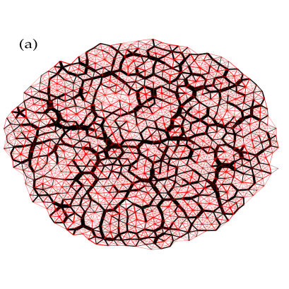
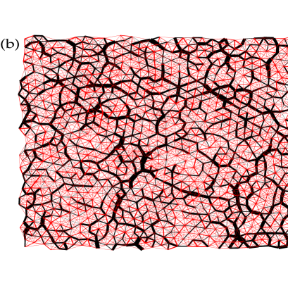
FIG. 1.: Representation of the network of quenched stresses in two small quenched Lennard-Jones particle systems in two dimensions: (a) a disk-shaped aggregate of diameter $2R\approx 32a$ containing $N=732$ particles (Protocol I) on the left and (b) a periodic bulk system with $L=32.9a$ and $N=1000$ (Protocol III) on the right hand side. The line scale is proportional to the tension transmitted along the links between beads. The black lines indicate repulsive forces (negative tensions), while the red links represent tensile forces between the verticies. Both shown networks are very similar despite different symmetries and quench protocols. They are strongly inhomogeneous and resemble the pattern seen in granular materials. Zones of weak attractive links appear to be embedded within the strong skeleton of repulsive forces.

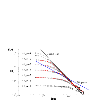
FIG. 2.: Correlations of frozen in forces for large periodic systems: (a) pair correlation $\langle cos^{2}(\tau)\rangle$ versus distance $r$. Here $\tau$ denotes either the angle between the directors $n_{i}$ and $n_{j}$ of the links $i$ and $j$ (symbols) or the angle between the director $n_{i}$ of link $i$ and the direction $n_{ij}$ between the links $i$ and $j$ (lines). The decay of the envelope is exponential with a length scale of the order of the mean bead size, hence, this does not introduce a new length scale. The dots correspond to an artificial force network obtained by shuffling randomly the tensions between existing links.(b) The number $N_{b}$ of boxes of size $b$ needed to cover the interactions transmitting repulsive tensions smaller than $t_{u}$. The curves do not differ much from box counting results on sets of randomly drawn links (dashed lines). Different slopes are included for comparison. The slope -1 corresponds to linear chain like structures, the -2 slope to a compact structure in 2D.

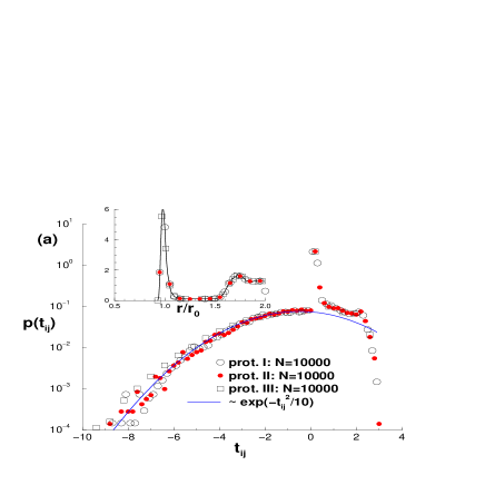
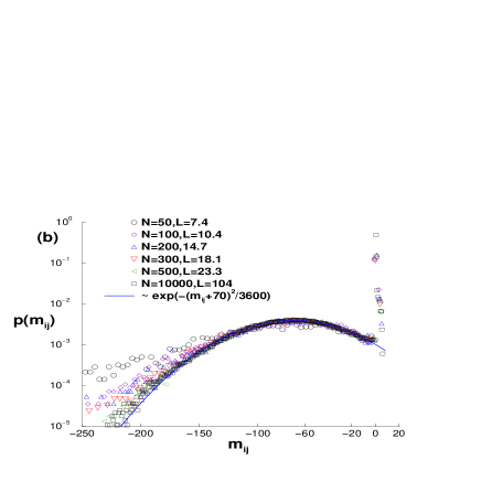
FIG. 3.: Histograms of contributions to the dynamical matrix: (a) comparison of the tension $t_{ij}$ for all three protocols at $N=10,000$. Inset: Histogram of distances $r_{ij}/r_{0}$ of interacting particles. (b) trace of matrix $m_{ij}=M_{xi,xj}+M_{yi,yj}$ for systems of various system sizes as indicated in the figure (protocol I). This demonstrates finite-size effects in the tail of the distributions of small systems with $L<20$ corresponding to an enhancement of the skeleton of very rigid contacts.

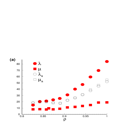
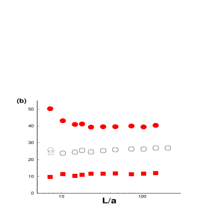
FIG. 4.: Lamé coefficients $\lambda$ and $\mu$ obtained for periodic bulk systems: (a) density variation for $N=10,000$, (b) size variation for $\rho=0.925$. Full symbols correspond to the direct measurement using Hooke’s law, open symbols are obtained using eqns. 12. Naturally, all Lamé coefficients rise with density as the number and strength of pair interactions increases. Note that while $\mu$ remains more or less constant $\lambda$ increases with decreasing $L$ in a similar way as pressure and particle energy (tab. III).

FIG. 5.: Comparison of non-affine displacement field $\delta\mbox{$\underline{u}$}(r)$ with eigenvector field $\delta\mbox{$\underline{v}$}_{p}(r)$ for periodic box of size $L=104a$ containing $N=10,000$ particles: (a) non-affine displacement field under elongation in $x$ direction, (b) same for plain shear using Lees-Edwards boundary conditions [32], (c) eigenvector field for $p=3$ and (d) eigenvector field for $p=7$. This confirms that the different noise fields are non-gaussian and are highly correlated in space and with respect to each other. Detailed inspection shows eddies like in turbulent flow.

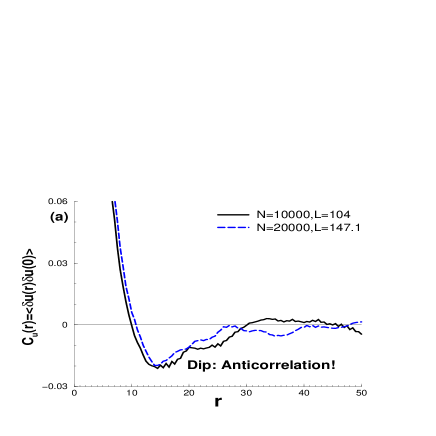
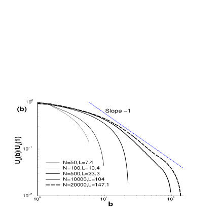
FIG. 6.: Characterization of non-affine displacement field $\delta u$-field obtained by simple elongation: (a) correlations function $C_{u}(r)=\langle\delta\mbox{$\underline{u}$}(r)\cdot\delta\mbox{$\underline{u}$}(0)\rangle$, (b) mean coarse-grained field $U_{x}(b)/U_{x}(b=1)$ versus the size $b$ of the coarse-graining. Both functions become system size independent for large $L$. The first figure on the left side shows clearly an anticorrelation in agreement with the eddies seen in the snapshot fig. 5(a).

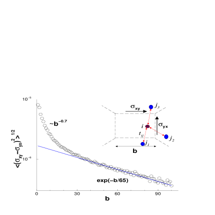
FIG. 7.: Asymmetry of the stress tensor of the forces generated in simple shear (Lees-Edwards boundary conditions) for a system containing 10 000 particles. We measure the ”microscopic stress“ acting on a volume element as shown in the sketch on the right. In the main figure we plot the average mean-squared stress difference $\langle(\sigma_{xy}-\sigma_{yx})^{2}\rangle^{1/2}$ versus the linear size $b$ of the volume element. For small box sizes $b<30a$ we evidence power law behavior which crosses to an exponential decay at large volume sizes.

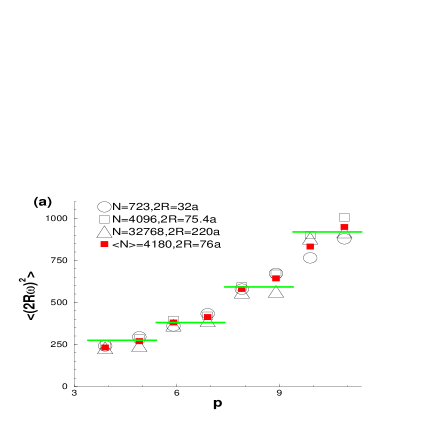
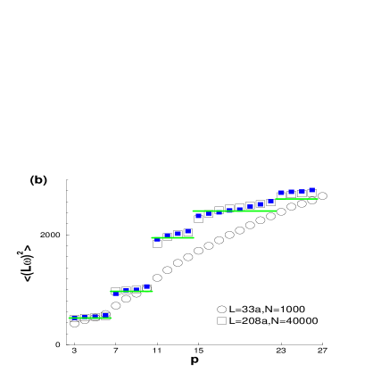
FIG. 8.: Comparison of the first non-trivial eigenvalues for (a) disk-shaped clusters and (b) bulk systems confirming the predicted degeneracies for sufficiently large samples. In small systems, the degeneracy is lifted. The frequencies are rescaled with the system size (as indicated) and compared with the theoretical predictions (horizontal lines). The open symbols in (a) correspond to the slow quench (Protocol I), the full symbols to a rapid quench (Protocol II) showing that the results of both protocols become similar for large disks. The open and full squares in (b) correspond to two different configurations with the same parameters.

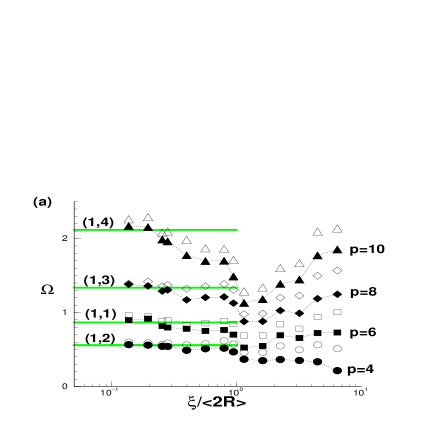
FIG. 9.: Finite-size scaling of reduced eigenfrequencies $\Omega(p,L)=\langle(\omega(p,L)L/2\pi c_{T})^{2}\rangle$ versus $\xi/L$ with $\xi\equiv 30a$ : (a) disk-shaped aggregates from protocol I with $L=2R$, (b) periodic bulk systems at $\rho=0.925$ (protocol III). The mode index $p$ increases from bottom to top, some of the $p$ are specifically given (full symbols). In both cases the degeneracy is systematically lifted for small systems and the continuum prediction (given by the horizontal lines) is approached non-monotoneously. The pairs of quantum numbers $(n,k)$ and $(n,m)$ associated with the predictions are indicated in figure (a) and (b) respectively.

FIG. 10.: First non-trivial eigenvectors (from $p=4$ up to $p=15$) of an aggregate of diameter $2R=120a$ containing $N=10,000$ particles (protocol I). We have indicated the running index $p$ and the pair of qantum numbers $(n,k)$. The two-fold degeneracy for $k>0$ is obvious. Note that each pair is rotated by a polar angle $\Delta\theta=\pi/2k$. The last mode represented is an axialsymmetric ‘breathing mode’ ($k=0$).

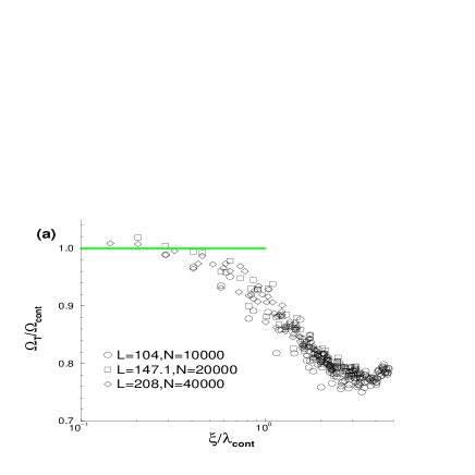
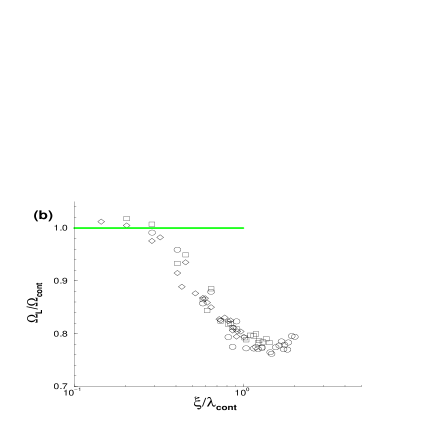
FIG. 11.: Scaling of (a) transverse and (b) longitudinal modes for different box sizes as indicated. The rescaled frequency $\Omega/\Omega_{cont}=\langle\omega^{2}\rangle/\omega_{cont}^{2}$ is plotted versus the inverse wave length $\xi/\lambda_{cont}$. The theoretically expected wave length $\lambda_{cont}=L/(n^{2}+m^{2})$ is given by the quantum numbers $(n,m)$ associated with the mode index $p$. We have again set $\xi\equiv 30a$. The crossover to continuum theory occurs at $\lambda\approx\xi$ for transverse modes and at about twice as large wave lengths for longitudinal modes. The success of both scaling plot suggests that $\xi$ is frequency independent for sufficiently large system sizes where $\lambda(p)\ll L$, but does depend the wave type. We regard this as the new central results of this paper.

FIG. 12.: Construction of noisy eigenvector field for periodic box configurations with $N=10,000,\rho=0.925$. Main figure: projection amplitude of empirical eigenvectors $p=3,11$ and $27$ on the theoretical plane waves which are indexed with $q$ with increasing frequency. Only the transverse modes are included for clarity. Insert: relative amplitude of noise as a function of wavelength $\lambda(p)$. The dotted line is a fit with $\exp(-\lambda_{cont}/30a)$ in agreement with the estimation $\xi\approx 30a$ for the characteristic wave length. The long-dashed line is a fit with $\lambda^{-2}$ in agreement with a scattering process.

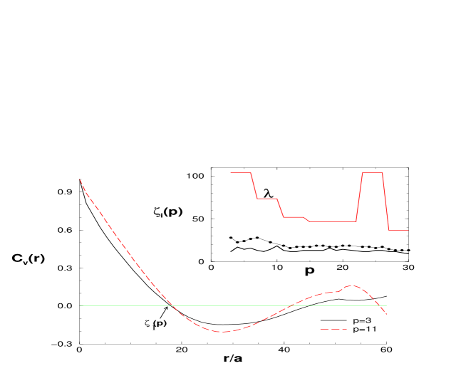
FIG. 13.: Correlation function $\langle\delta\mbox{$\underline{v}$}_{p}(r)|\delta\mbox{$\underline{v}$}_{p}(0)\rangle$ of the eigenvector noise fields for $p=3$ and $11$ versus distance $r$. The curves are similar to the ones shown in fig. 6(b) and feature again prominent anti-correlations. Inset: $\zeta_{1}(p)$ characterizing the anti-correlation for N=10 000 (dotted line) and N=5 000 (bold line). Also included is the wavelength from Eq. 6 associated with each continuum mode (top line).