Superconductivity in carbon nanotube ropes

Abstract

We investigate the conditions in which superconductivity may develop in ropes of carbon nanotubes. It is shown that the interaction among a large number of metallic nanotubes favors the appearance of a metallic phase in the ropes, intermediate between respective phases with spin-density-wave and superconducting correlations. These arise in samples with about 100 metallic nanotubes or more, where the long-range Coulomb interaction is very effectively reduced and it may be overcome by the attractive interaction from the exchange of optical phonons within each nanotube. We estimate that the probability for the tunneling of Cooper pairs between neighboring nanotubes is much higher than that for single electrons in a disordered rope. The effect of pair hopping is therefore what establishes the intertube coherence, and the tunneling amplitude of the Cooper pairs dictates the scale of the transition to the superconducting state.

]

I Introduction

During the last years there has been growing evidence of the existence of superconducting correlations in carbon nanotubes. In the first place, the proximity effect has been observed in ropes of nanotubes placed between superconducting contacts[1, 2]. Quite remarkably, it has been shown that the nanotubes may support supercurrents below the critical temperature of the contacts[1]. Later on, there have been experiments directed to probe the superconductivity inherent to the nanotubes[3]. In some of the ropes, a transition has been observed at a temperature below $1\;{\rm K}$, with a drop of two orders of magnitude in the resistance down to a value consistent with the finite number of channels in the rope.

From a theoretical point of view, the electronic interactions in the nanotubes have been also the subject of much attention[4, 5, 6, 7]. The nanotubes may show metallic properties depending on the helicity with which the graphene sheet is wrapped to form the tubule. The experimental results[8] have agreed on that point with the theoretical predictions[9]. Given that the conduction takes place in a one-dimensional (1D) structure, it has been proposed that the nanotubes should be ideal systems for the observation of the so-called Luttinger liquid behavior[10, 11, 12, 13]. Actually, there have been measurements providing evidence of the power-law dependence of the tunneling conductance[14, 15], what is a signature of the mentioned behavior. These experiments seem therefore to probe a regime in which the repulsive Coulomb interaction turns out to be dominant in the nanotubes.

On the other hand, the interaction with the elastic modes of the nanotube plays an important role in the development of the superconducting correlations[16]. The magnitude of the supercurrents measured in Ref. [1] is in some instances up to 40 times larger than expected from the estimate within the conventional proximity effect. It has been shown that the temperature dependence of the supercurrents is characteristic of the 1D behavior of the system. Moreover, their values can be only explained by taking into account the attractive electronic interaction coming from the exchange of phonons, on top of the repulsive Coulomb interaction[16].

Recently, a microscopic model has been elaborated to account for the observation of superconductivity intrinsic to the ropes of nanotubes[17]. In these systems, the Coulomb interaction can be significantly reduced depending on the number of metallic nanotubes in the rope. One has to incorporate therefore the balance between the repulsive electron interaction and the effective attractive interaction coming from phonon exchange. It has been shown that, in the case of samples with about 300 nanotubes like those displayed in Ref. [3], the superconducting correlations prevail in the system. The intertube coherence is established mainly through the tunneling of Cooper pairs, which gives rise to the superconductivity in the bulk under suitable conditions[17].

One of the aims of the present paper is to unveil the different phases that arise in the competition between the repulsive Coulomb interaction and the attractive interaction from phonon exchange in the ropes of nanotubes. For this purpose we will map the phase diagram of these systems taking the strength of the phonon couplings and the number of metallic nanotubes as the relevant variables. We will show that the region where the superconductivity may develop opens up for relatively large contents of metallic nanotubes. The phase with spin-density-wave correlations characteristic of a repulsive interaction is confined to the cases where there are only a few nanotubes in the rope.

We assume in any event that the formation of spin or charge order in the bulk is prevented by the fact that the nanotubes have a random distribution of helicities in the ropes. These do not have a crystalline structure from the three-dimensional point of view, and the only possible long-range order arises in the superconducting phase. We will see that, between the phases with superconducting and spin-density-wave correlations, there is a metallic phase with no signal of instability in any direction. This is the phase to be found out most likely when measuring ropes with a number below $\sim 100$ metallic nanotubes.

We will also address the question of the maximum transition temperature that can be reached in the ropes. There have been recent experimental measures in carbon nanotubes of minimum diameter inserted in a zeolite matrix, from which a critical temperature of about $15\;{\rm K}$ has been inferred[18]. The small radius and high curvature of those nanotubes have to lead to an enhancement of the electron-phonon coupling. This would explain in turn the increase in the critical scale for superconductivity.

One has to bear in mind, however, that the correlations in individual nanotubes provide an indirect measure of the superconducting state. We will show that, in the three-dimensional structure of the rope, the transition temperature is dictated by the amplitude for the Cooper pairs to tunnel between neighboring nanotubes. Even in samples with large number of metallic nanotubes, the opening of the superconducting phase depends at last on the existence of intertube coherence. The most efficient way to increase the transition temperature may come actually from devising some mechanism to enhance the tunneling rate of the Cooper pairs between the nanotubes.

The content of this paper is organized as follows. In Section II we analyze the origin of the different interactions in the individual nanotubes. Section III is devoted to elaborate the model that takes into account the interaction among the metallic nanotubes, ending up with the discussion of the possible phases of a rope. In Section IV we incorporate the effect of the tunneling of the Cooper pairs, performing some estimates of the transition temperature under different conditions. Finally, Section V is devoted to discuss some of the assumptions under which our general analysis applies.

II Electron interactions in carbon nanotubes

We begin by considering the band structure of the individual metallic nanotubes. We focus on the so-called armchair nanotubes, which have the structure depicted in Fig. 10 of the Appendix A. They have gapless subbands irrespective of the influence of the nanotube curvature on the orbitals. Fig. 1 represents for instance the spectrum of a (10,10) armchair nanotube, which has a radius $R\approx 15a/\pi$ in terms of the carbon-carbon distance $a$. We will concentrate on the case of undoped nanotubes, in which the Fermi level is placed at $E=0$ in the scale of the figure.

FIG. 1.: Different subbands of a (10,10) armchair nanotube. The energy $E$ is measured in units of the hopping parameter $t$ and the momentum $k$ is in units of the inverse of the lattice spacing.

The most important feature for the study of the low-energy properties is the crossing of two subbands at the Fermi level, that we label with the indices 1 and 2 as shown in the figure. These subbands correspond to the modes with vanishing transverse momentum in the nanotube, which are governed by the one-particle hamiltonian[19]

$${\cal H}=t\left(\begin{array}[]{cc}0&1-2\cos(\sqrt{3}ka/2)\\ 1-2\cos(\sqrt{3}ka/2)&0\end{array}\right)$$ (1)

$t$ being the hopping amplitude between neighboring sites.

The amplitudes of the modes behave differently in the nanotube lattice depending on whether they belong to one or the other subband. In the case of the subband with bonding character, the amplitude is a smooth function of the position, while the modes in the other subband have an amplitude that alternates the sign between the two sublattices of the honeycomb lattice. This property has important consequences regarding the form of the electron-electron interactions as well as the coupling of the electrons to the elastic modes of the lattice.

In what follows we undertake the analysis of the low-energy regime in which the physical properties are dominated by the branches with approximate linear dispersion near the Fermi level. For this purpose, we introduce an energy cutoff $E_{c}$ below the energy of the bottom of the first unoccupied subband, together with its counterpart $-E_{c}$ below the Fermi level. The different branches are labelled by an index $r=\pm$ denoting the right or left-moving character, and by the Fermi point $i=\pm$ to which they are attached, as shown in Fig. 2. Correspondingly, we end up with a collection of electron fields $\Psi_{ri\sigma}(x)$, to which one more index $a$ will be added later on to label the nanotube in the rope.

FIG. 2.: Linear branches in the low-energy spectrum of a carbon nanotube.

The electron interactions that we are going to consider have in general the form

$$\int_{-k_{c}}^{k_{c}}dk\int_{-k_{c}}^{k_{c}}dp\int_{-k_{c}}^{k_{c}}dq\;\;\;\;\;\;\;\;\;\;\;\;\;\;\;\;\;\;\;\;\;\;\;\;\;\;\;\;\;\;$$ (2)

$$\Psi_{ri\sigma}^{\dagger}(p+k)\Psi_{sj\sigma}(p)V(k)\Psi_{tk\sigma^{\prime}}^{\dagger}(q-k)\Psi_{ul\sigma^{\prime}}(q)$$ (3)

The processes between the different branches can be cataloged according to the notation of Ref. [5]. They fall into 12 different classes with respective couplings denoted by $g_{i}^{(j)}$, the indices taking the values $i=1,2,4$ and $j=1,\ldots 4$. The lower label pays attention to the Fermi points of the respective fields, following the convention that assigns $i=1$ to backscattering processes, $i=2$ to scattering between currents at different Fermi points, and $i=4$ to scattering between currents at the same Fermi point. The upper label follows the same rule classifying the different combinations of left-movers and right-movers, including the possibility of having Umklapp processes ($j=3$).

We analyze next the contributions to the different scattering processes from the interactions present in the nanotubes.

Electron-electron interactions.

We deal with the situation in which the Coulomb interaction is not screened by external gates. It is known that the Coulomb potential remains long-ranged in one spatial dimension[20]. The appropriate expression in momentum space is[21]

$$V_{C}(k)=(e^{2}/4\pi^{2})\log|(k_{c}+k)/k|$$ (4)

The repulsive interaction is therefore enhanced at small momentum transfer, as in the processes shown in Fig. 3. However, processes like those in Fig. 4, in which the flavor $r$ is changed by the interaction, are highly suppressed. This is due to the fact that, as mentioned before, the modes corresponding to one of the gapless subbands alternate the sign in the two sublattices of the nanotube. When the distance between the two currents that interact is much larger than the nanotube radius, the matrix element of the interaction averages to zero over the section of the nanotube.

FIG. 3.: Small momentum-transfer processes which are enhanced by the long-range Coulomb interaction.

Thus, the long-range repulsive interaction reflects in an enhancement of the interbranch and intrabranch couplings $g_{2}^{(2)}$, $g_{2}^{(4)}$, $g_{4}^{(2)}$ and $g_{4}^{(4)}$. The flavor-changing processes associated to $g_{2}^{(1)}$, $g_{2}^{(3)}$, $g_{4}^{(1)}$ and $g_{4}^{(3)}$ survive in the form of a residual short-range interaction. Its strength, however, is corrected by a factor of the order of $\sim 0.1\;a/R$ in comparison to the nominal strength of the long-range Coulomb interaction[6, 7]. This represents in general a relative reduction by two orders of magnitude, for the nanotubes that are typically found in the ropes.

FIG. 4.: Flavor-changing processes with small contribution from the Coulomb interaction.

There remain the processes with momentum transfer of the order of $\sim 2k_{F}$. These processes probe the interaction at short distances. It has been shown that the corresponding couplings are also reduced by a factor of the order of $\sim 0.1\;a/R$ relative to the strength $e^{2}/4\pi^{2}$ of the forward-scattering processes[6, 7].

The couplings for large momentum transfer, as well as $g_{2}^{(1)}$, $g_{2}^{(3)}$, $g_{4}^{(1)}$ and $g_{4}^{(3)}$, are marginally relevant in the renormalization group sense. This means that they have greater strength as the theory is scaled to smaller energies, but the rate of increase starts being quadratic in the own couplings[5, 6]. Thus, one has to proceed to extremely low energies, many orders of magnitude below $E_{c}$, to have a significant increase of the couplings with respect to their nominal values[6].

Electron-phonon interactions.

The electron-phonon interactions give rise to a retarded interaction between the electrons, which may become attractive at frequencies below the typical energy of the phonons. The potential for the effective interaction has the form

$$V(k,\omega)=-g_{p,p^{\prime}}(k)g_{q,q^{\prime}}(k)\frac{\omega_{k}}{-\omega^{2}+\omega_{k}^{2}}$$ (5)

where $\omega_{k}$ is the phonon energy and the $g_{p,p^{\prime}}(k)$ are appropriate electron-phonon couplings described in the Appendix A. The form of the interaction is dictated by the latter, whose dependence on the momentum transfer varies according to the kind of phonons exchanged.

Acoustic phonons.— In this case, $\omega_{k}$ is proportional to $|k|$ at small momentum transfer. This means that, regarding the interbranch and intrabranch processes, the range of energies in which the effective interaction becomes attractive is greatly reduced. This instance has been studied with detail in Ref. [22], looking for the regime in which the retarded interaction may drive the transition to a state with superconducting correlations. Taking the parameters appropriate for the nanotubes, it can be seen that the critical exponents estimated in this way are very small. Therefore, the acoustic phonons at small momentum transfer do not play a role in the superconductivity observed in the nanotubes.

Moving now to the processes with large momentum transfer $k\sim 2k_{F}$, the phonon energy $\omega_{2k_{F}}$ becomes of the order of the Debye frequency $\omega_{D}$. This provides then a significant range in which the effective interaction becomes attractive. The precise couplings to the acoustic phonons in the nanotubes can be found in Ref. [23]. It has been shown there that some restrictions arise in the exchange of phonons depending on the bonding or antibonding character of the subbands involved. In the case of longitudinal acoustic phonons, the processes cannot take one electron from a given subband to the other. Moreover, the couplings have opposite signs when the scattered electron is in one or the other subband. The exchange of phonons leads then to the effective couplings below the Debye frequency

$$g_{{\rm eff},1}^{(1)}=-g_{{\rm eff},1}^{(3)}<0$$ (6)

In the case of the transverse acoustic phonons, the phonon-exchange processes in which the electrons remain in the same subband are forbidden. Processes associated to $g_{1}^{(2)}$ and $g_{1}^{(4)}$ in which the electron shifts from one subband to the other could play in principle a role, but there is a kinematic factor that vanishes when the incoming and outgoing modes have opposite momenta. There are therefore no more contributions from the acoustic phonons when the system is precisely at half-filling.

Optical phonons.— The Debye frequency is of the same order that the energy of the acoustic phonons at $2k_{F}$, so that we can expect the effective couplings to be comparable to those in Eq. (6). The different symmetry of the modes with bonding and antibonding character imposes again restrictions in the way the optical phonons can be exchanged, as shown in the Appendix A. In the case of the transverse optical phonons, the electron modes have to remain within the same subband, while the longitudinal phonons force the electron to shift from one of the subbands to the other. The effective couplings that we get have the following signs

$$g_{{\rm eff},2}^{(1)} = -g_{{\rm eff},2}^{(3)}<0$$ (7)

$$g_{{\rm eff},2}^{(2)} = -g_{{\rm eff},2}^{(4)}<0$$ (8)

$$g_{{\rm eff},4}^{(1)} = -g_{{\rm eff},4}^{(3)}<0$$ (9)

$$g_{{\rm eff},4}^{(4)} = -g_{{\rm eff},4}^{(2)}<0$$ (10)

We finally remark that the Debye frequency of the phonons in the nanotubes can be estimated to be between 0.1 and $0.2\;{\rm eV}$. This is of the same order of magnitude that the cutoff $E_{c}$, that marks the energy below which the nanotubes can be viewed as simple 1D systems. In that regime, the effective interactions coming from the exchange of phonons can be matched against the interaction of purely electronic origin. We will adopt henceforth this procedure, as long as the electronic properties in which we are going to be interested refer to energies much lower than $E_{c}$.

III Electronic interactions in ropes of nanotubes

We turn now to the processes that take place between the nanotubes in a rope. A property to be taken into account is that the rope is made of a disordered mixture of nanotubes with all kind of diameters and helicities. Given their random distribution, the lattices of neighboring nanotubes are not aligned in general. The consequences of this fact have been studied in Ref. [24]. As long as there is a mismatch in the position of the respective Fermi points of neighboring nanotubes, the conservation of the longitudinal momentum cannot be precisely enforced in the tunneling processes. At the one-particle level, the electronic states appear to be localized along the individual nanotubes, and the intertube coherence is strongly suppressed.

The authors of Ref. [24] have computed the expression of the tunneling amplitude between nanotubes in the so-called compositionally disordered ropes. In the case of nanotubes with the same helicity and aligned lattices, the estimate for the tunneling amplitude is $t_{T}\sim 0.01\;{\rm eV}$. When there is a mismatch $\delta k$ between the Fermi points of neighboring nanotubes, it has been found that the amplitude for an electron hopping between them is suppressed by a relative factor $\sim\exp[-Ra_{0}(\delta k)^{2}/4]$, where $a_{0}$ is a parameter of the order of $\sim 0.5$ Å. Taking a typical nanotube radius $R=7$ Å, the average value of that factor is of the order of $\sim 0.005$.

The presence of compositional disordered has also important consequences regarding the kind of electronic instabilities that may develop in the rope. Depending on the point of the phase diagram, the individual nanotubes may support $2k_{F}$ charge-density-wave and superconducting correlations, or $2k_{F}$ spin-density-wave correlations. It is clear, however, that the absence of a three-dimensional crystalline structure precludes the development of charge or spin order in the bulk of the rope. The transition to a superconducting state is therefore favored when the correlations are strong enough to force the symmetry breaking in that direction.

The possibility of having a superconducting transition in the rope of nanotubes arises from the balance of the effective attractive interactions due to phonon exchange and the repulsive interactions of purely electronic character. At the diagrammatic level, for instance, the correlations with $s$-wave order parameter are driven by the couplings $g_{2}^{(2)}$, $g_{1}^{(1)}$, $g_{2}^{(1)}$ and $g_{1}^{(2)}$, as shown in the Appendix B [25]. The obstruction to having superconducting correlations in the nanotubes comes, in principle, from the large contribution of the Coulomb potential to the coupling $g_{2}^{(2)}$. In this respect, the processes associated to $g_{1}^{(1)}$ and $g_{2}^{(1)}$ contribute to enhance the superconducting correlations when they are able to develop, but they play a secondary role in the determination of the phase diagram of the ropes.

It is therefore necessary to build a model that takes into account the competition between attractive and repulsive interactions in the interbranch and intrabranch processes $g_{2}^{(2)}$, $g_{2}^{(4)}$, $g_{4}^{(2)}$ and $g_{4}^{(4)}$. This model can be solved by means of bosonization techniques. With this method, one boson field is introduced for each of the linear branches below $E_{c}$ in each metallic nanotube. At this point we need to introduce a new index $a$ labelling the metallic nanotubes in the rope, so that the fermion fields read now $\Psi^{(a)}_{ri\sigma}(x)$. The correspondence between each of these and the respective boson operator is given by

$$:\Psi^{(a)\dagger}_{ri\sigma}(x)\Psi^{(a)}_{ri\sigma}(x):=\rho^{(a)}_{ri\sigma}(x)$$ (11)

where the colons represent normal ordering and $\rho^{(a)}_{ri\sigma}(x)$ stands for the density operator associated to the given branch.

Neglecting for the time being the tunneling between the nanotubes, the hamiltonian for the model, including a collection $a=1,\ldots n$ of metallic nanotubes, takes the form

$$H_{0} = \frac{1}{2}v_{F}\int_{-k_{c}}^{k_{c}}dk\sum_{ari\sigma}:\rho^{(a)}_{ri\sigma}(k)\rho^{(a)}_{ri\sigma}(-k):$$ (13)

$$+\frac{1}{2}\int_{-k_{c}}^{k_{c}}dk\;\sum_{ari\sigma}\rho^{(a)}_{ri\sigma}(k)\;\sum_{bsj\sigma^{\prime}}V^{(ab)}_{ri,sj}(k)\;\rho^{(b)}_{sj\sigma^{\prime}}(-k)$$

where $k_{c}$ is related to $E_{c}$ through the Fermi velocity $v_{F}$, $k_{c}=E_{c}/v_{F}$.

The interaction term in (13) can be better organized by introducing the charge density operators

$$\rho^{(a)}_{ri\rho}(x)=\frac{1}{\sqrt{2}}\left(\rho^{(a)}_{ri\uparrow}(x)+\rho^{(a)}_{ri\downarrow}(x)\right)$$ (14)

and their spin density counterparts. We define further the linear combinations

$$\tilde{\rho}^{(a)}_{1\rho}(x) = \rho^{(a)}_{++\rho}(x)+\rho^{(a)}_{--\rho}(x)$$ (15)

$$\tilde{\rho}^{(a)}_{2\rho}(x) = \rho^{(a)}_{+-\rho}(x)+\rho^{(a)}_{-+\rho}(x)$$ (16)

Obviously, $\tilde{\rho}^{(a)}_{1\rho}(x)$ is made of the modes with bonding character, while $\tilde{\rho}^{(a)}_{2\rho}(x)$ contains those with antibonding character.

We recall that, in the case of the attractive interaction from the exchange of phonons, the sign of the coupling depends on the bonding or antibonding character of the currents involved. Thus, a great simplification is achieved by introducing the operators

$$\tilde{\rho}^{(a)}_{+\rho}(x) = \frac{1}{\sqrt{2}}\left(\tilde{\rho}^{(a)}_{1\rho}(x)+\tilde{\rho}^{(a)}_{2\rho}(x)\right)$$ (17)

$$\tilde{\rho}^{(a)}_{-\rho}(x) = \frac{1}{\sqrt{2}}\left(\tilde{\rho}^{(a)}_{1\rho}(x)-\tilde{\rho}^{(a)}_{2\rho}(x)\right)$$ (18)

The Coulomb interaction acts on the symmetric combinations $\tilde{\rho}^{(a)}_{+\rho}(x)$, while the effective attractive interaction only couples the antisymmetric combinations $\tilde{\rho}^{(a)}_{-\rho}(x)$. The hamiltonian (13) can be rewritten in the form

$$H_{0} = \frac{1}{2}v_{F}\int_{-k_{c}}^{k_{c}}dk\sum_{ari\sigma}:\rho^{(a)}_{ri\sigma}(k)\rho^{(a)}_{ri\sigma}(-k):$$ (21)

$$+\frac{1}{2}\int_{-k_{c}}^{k_{c}}dk\;\left(\sum_{a}\tilde{\rho}^{(a)}_{+\rho}(k)\;V_{C}(k)\sum_{b}\;\tilde{\rho}^{(b)}_{+\rho}(-k)\right.$$

$$\left.\;\;\;\;\;\;\;\;\;\;\;\;\;\;\;\;\;\;+g\sum_{a}\tilde{\rho}^{(a)}_{-\rho}(k)\;\tilde{\rho}^{(a)}_{-\rho}(-k)\right)$$

where we have defined

$$g=g_{2}^{(2)}=g_{4}^{(4)}=-g_{2}^{(4)}=-g_{4}^{(2)}$$ (22)

After the decoupling of the Coulomb and the effective attractive interaction, we observe that the latter affects to a number $n$ of the $4n$ density operators, while the Coulomb interaction acts only on the channel of the total charge density. That is, the hamiltonian (21) can be completely diagonalized by changing variables to the symmetric combination of the charge density operators of all the metallic nanotubes. This is a consequence of the long-range character of the Coulomb interaction, that allows us to assume that, in the interbranch and intrabranch processes, the different nanotubes interact between them with the same strength.

The balance between the long-range repulsive interaction and the effective attractive interaction is possible as the former turns out to be greatly reduced for large values of $n$. The attraction from phonon exchange is otherwise an intratube effect that does not depend on the number of nanotubes. It is then interesting to draw the phase diagram of the ropes in terms of the number of metallic nanotubes and the strength of the attractive interaction. At large values of $n$ and sufficiently large values of $|g|$, there must exist a phase where the attractive interaction prevails, with the development of superconducting correlations in the individual nanotubes. For low values of $n$ and small $|g|$, the electronic properties have to be dictated by the Coulomb interaction, with the appearance of the spin-density-wave correlations characteristic of the Luttinger liquid behavior.

The different phases can be identified by looking at the correlators of the model. The bosonization techniques allow to compute them by using the correspondence between the fermion fields and the respective boson operators[10, 11]

$$\Psi^{(a)}_{r+\sigma}(x) = \exp\left(i\Phi^{(a)}_{r+\sigma}(x)\right)$$ (23)

$$\Psi^{(a)}_{r-\sigma}(x) = \exp\left(-i\Phi^{(a)}_{r-\sigma}(x)\right)$$ (24)

where $\partial_{x}\Phi^{(a)}_{ri\sigma}(x)=2\pi\rho^{(a)}_{ri\sigma}(x)$ .

We deal first with the propagator $D_{\rm sc}^{(0)}(x,t)$ of the Cooper pairs in the individual nanotubes. This object factorizes into the different channels that appear after diagonalizing the hamiltonian

$$D_{\rm sc}^{(0)}(x,t) \equiv \langle\Psi^{(a)\dagger}_{++\uparrow}(x,t)\Psi^{(a)\dagger}_{--\downarrow}(x,t)\Psi^{(a)}_{--\downarrow}(0,0)\Psi^{(a)}_{++\uparrow}(0,0)\rangle$$ (25)

$$= C_{\rm sc}(x,t)\prod_{1}^{n}N_{\rm sc}(x,t)\prod_{1}^{3n-1}F(x,t)$$ (26)

The first factor corresponds to the channel of the total charge density of the metallic nanotubes, while $N_{{\rm sc}}$ stands for the contribution of the antisymmetric combination of the charge in the two subbands. The rest of the factors corresponds to the channels with no interaction.

The different factors in Eq. (26) can be computed in terms of the respective boson propagators, what leads to expressions of the form

$$X_{\rm sc}(x,t) = \exp\left(-\frac{1}{2n}\int_{0}^{k_{c}}dk\;\;\;\;\;\;\;\;\;\;\;\;\;\;\;\;\;\;\right.$$ (28)

$$\;\;\;\;\;\;\;\;\;\left.\frac{1}{\mu(k)\>k}\left(1-\cos(kx)\>\cos(\tilde{v}_{F}kt)\right)\right)$$

In the case $X_{\rm sc}(x,t)=C_{\rm sc}(x,t)$, we have $\mu(k)=1/\sqrt{1+8nV_{C}(k)/v_{F}}$ and $\tilde{v}_{F}(k)=v_{F}/\mu(k)$. For $X_{\rm sc}(x,t)=N_{\rm sc}(x,t)$, we have the constant parameters $\mu=1/\sqrt{1-4|g|/\pi v_{F}}$ and $\tilde{v}_{F}=v_{F}/\mu$.

The same technique can be applied to the computation of the propagator $D_{\rm sdw}^{(0)}(x,t)$ of the spin-density-waves along the nanotubes. The correlator is given by

$$D_{\rm sdw}^{(0)}(x,t) \equiv \langle\Psi^{(a)\dagger}_{++\uparrow}(x,t)\Psi^{(a)}_{--\downarrow}(x,t)\Psi^{(a)\dagger}_{--\downarrow}(0,0)\Psi^{(a)}_{++\uparrow}(0,0)\rangle$$ (29)

$$= C_{\rm sdw}(x,t)\prod_{1}^{n}N_{\rm sdw}(x,t)\prod_{1}^{3n-1}F(x,t)$$ (30)

Each of the factors in Eq. (30) has now the representation

$$X_{\rm sdw}(x,t) = \exp\left(-\frac{1}{2n}\int_{0}^{k_{c}}dk\;\;\;\;\;\;\;\;\;\;\;\;\;\;\;\;\;\;\right.$$ (32)

$$\;\;\;\;\;\;\;\;\;\left.\frac{\mu(k)}{k}\left(1-\cos(kx)\>\cos(\tilde{v}_{F}kt)\right)\right)$$

with the same correspondence between $\mu(k)$ and $C$, $N$ and $F$ as for the propagator of the Cooper pairs.

The correlators in the individual nanotubes cannot display an instability for any finite value of the frequency[13]. The way to discern the tendency to the formation of long-range order is to determine whether the correlations are enhanced at large distances over the values in the absence of interaction. When this happens, the Fourier transform of the corresponding propagator at zero temperature diverges at zero frequency and momentum. At nonvanishing temperature, the propagators remain finite but the intertube coupling may give rise to the breakdown of the symmetry if the correlations in the nanotubes are sufficiently enhanced. We will address this question in the next section. The computation of the propagators (26) and (30) can be extended to the case of temperature $T\neq 0$, just by inserting the factor $1+2/[\exp(\tilde{v}_{F}|k|/T)-1]$ in the integrand of expressions such as (28) and (32) [10].

At this point, we stick to the model at zero temperature and map the regions with enhanced superconducting or spin-density-wave correlations. The propagators (26) and (30) do not show a perfect scaling behavior at large distances, due to the momentum dependence of the Coulomb potential. We may take however an effective value $k_{0}$ of the momentum in the infrared to approximate the behavior of each propagator by a power-law with a constant exponent.

In the case of $D_{\rm sc}^{(0)}(x,t)$, the decay at large distances takes the form

$$D_{\rm sc}^{(0)}(x,0)\sim 1/x^{2+\gamma}$$ (33)

where the anomalous scaling dimension is given by

$$\gamma=\frac{1}{2n\mu(k_{0})}+\frac{1}{2\mu}-\frac{1}{2}-\frac{1}{2n}$$ (34)

Similarly, $D_{\rm sdw}^{(0)}(x,t)$ has a large-distance behavior

$$D_{\rm sdw}^{(0)}(x,0)\sim 1/x^{2+\delta}$$ (35)

with an anomalous exponent

$$\delta=\frac{\mu(k_{0})}{2n}+\frac{\mu}{2}-\frac{1}{2}-\frac{1}{2n}$$ (36)

We have represented in Fig. 5 the different phases that arise by varying the number $n$ of metallic nanotubes and the strength $|g|$ of the intratube attractive interaction. For the Coulomb interaction, we have taken the values $2e^{2}/\pi^{2}v_{F}=1.0$ and $k_{0}=10^{-3}k_{c}$, which are appropriate for typical experimental samples[16]. At sufficiently large values of $n$, a phase with superconducting correlations opens up, characterized by negative values of the anomalous dimension $\gamma$. This phase is placed above the upper full line in the diagram. Another phase with spin-density-wave correlations shows up, below the lower full line in the diagram. This region corresponds to the points characterized by negative values of $\delta$.

FIG. 5.: Phase diagram showing the regions where the superconducting (SC) correlations and the spin-density-wave (SDW) correlations prevail, in terms of the strength $|g|$ of the effective attractive interaction and the number $n$ of metallic nanotubes.

We observe also the existence of an intermediate region in which neither $\gamma$ nor $\delta$ are negative. This represents a phase with intrinsic metallic properties, where no correlations are enhanced and no order would develop irrespective of the value of the intertube coupling in the rope[26]. In our model, this phase arises from the balance between the Coulomb and the effective attractive interaction. The former remains long-ranged, but the interaction among a large number of metallic nanotubes is what favors the appearance of the metallic phase, as a bridge to the development of the superconducting correlations.

IV Superconducting transition in ropes of nanotubes

In the preceding section we have neglected the effect of tunneling between metallic nanotubes, relying on the smallness of the amplitude for that process. We have seen however that, in the absence of intertube hopping, the model cannot develop any instability at finite temperature. In this respect, the upper full line in Fig. 5 has to be considered as a first approximation to the boundary where the superconducting phase opens up in real samples. The tunneling amplitude between neighboring nanotubes in a rope is actually what dictates the transition temperature to the superconducting state, as we study in what follows.

As mentioned before, the single-particle hopping between neighboring nanotubes is strongly suppressed in a disordered rope. The tunneling amplitude between nanotubes with different helicities can be estimated to be of the order of $\sim 0.5\times 10^{-4}\;{\rm eV}$. Its smallness stems from the obstruction to having precise momentum conservation in the hopping between the misaligned lattices of the nanotubes[24]. In these conditions, the tunneling of Cooper pairs turns out to be a much more important effect.

The probabilities of the single-particle hopping and the pair hopping can be compared by measuring the respective amplitudes with respect to the energy cutoff $E_{c}$. We can take this quantity of the order of $\sim 0.1\;{\rm eV}$, which is the scale below which the nanotubes in a rope are seen as 1D objects. Thus, we find that the single-particle hopping has a relative weight of the order of $\sim 0.5\times 10^{-3}$. The amplitude for the tunneling of Cooper pairs can be computed roughly as the square of the amplitude $t_{T}\sim 0.01\;{\rm eV}$, so that the relative weight $\lambda_{2}$ of that process becomes of the order of $\sim 10^{-2}$.

The model of the preceding section has to be corrected then by adding to the hamiltonian (21) the term describing the tunneling of the Cooper pairs

$$H_{2}=\sum_{\langle a,b\rangle}(\lambda_{2})_{ab}\int_{-k_{c}}^{k_{c}}dk\int_{-k_{c}}^{k_{c}}dp\int_{-k_{c}}^{k_{c}}dp^{\prime}\;\;\;\;\;\;\;\;\;\;\;\;\;\;\;\;\;\;\;\;$$ (37)

$$\Psi^{(a)\dagger}_{ri\uparrow}(k+p)\Psi^{(a)\dagger}_{-r-i\downarrow}(-p)\Psi^{(b)}_{-s-j\downarrow}(-p^{\prime})\Psi^{(b)}_{sj\uparrow}(k+p^{\prime})$$ (38)

where the sum runs over all pairs $\langle a,b\rangle$ of nearest-neighbor metallic nanotubes.

Given that the model without pair hopping is exactly solvable, we can compute the scaling dimension of the operator in $H_{2}$. We can check in this way whether this is a relevant perturbation or otherwise it fades away at low energies. The naïve dimension of the four-fermion operator is 2, and the deviation from that value can be obtained from the large-distance behavior of the correlator in Eq. (26). The anomalous scaling dimension coincides with the exponent given in Eq. (34). Therefore, we observe that it is negative in the phase with superconducting correlations, what points at the enhancement of the pair-hopping perturbation at low energies.

The values that can be obtained for $\gamma$ are rather small anyhow. Taking again an effective value of $k_{0}=10^{-3}k_{c}$ , we find $\gamma\approx-0.02$ for $n=60$ and $4|g|/\pi v_{F}=0.6$, and $\gamma\approx-0.16$ for $n=120$ and $4|g|/\pi v_{F}=0.8$. In the latter case, for instance, the anomalous scaling leads to an enhancement by a factor that, four orders of magnitude below $E_{c}$, can be at most of the order of $(10^{-4})^{\gamma}\sim 4$. Such a scaling does not affect our estimate of the order of magnitude for the relative weight $\lambda_{2}$.

As long as we have the small parameter $\lambda_{2}$ in the system, we may include the effects of pair hopping by summing up all the processes in which a Cooper pair, propagating along a nanotube with the amplitude (26), tunnels to a neighboring metallic nanotube. Let us denote by $l_{a}$ the position of nanotube $a$ in the transverse section of the rope. We will assume that the metallic nanotubes are dense in the collection of nanotubes of the rope[27]. Then, we may write the propagator of the Cooper pairs between the metallic nanotube $a$ and the metallic nanotube $b$ as a function $D(l_{a},l_{b};x,t)$. This object is related to $D_{\rm sc}^{(0)}(x,t)$ through the self-consistent equation represented in Fig. 6, in the approach that takes $H_{2}$ as a perturbation to the hamiltonian (21).

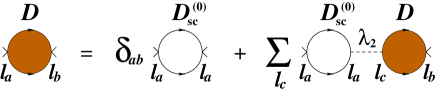
FIG. 6.: Self-consistent diagrammatic equation for the propagator $D$ of Cooper pairs along the rope.

For the sake of simplifying the calculation, we will suppose that the positions $l_{a}$ form a periodic arrangement in the transverse section of the rope. Then we can take the Fourier transform of these variables as well as of the distance $x$ along the nanotube. The equation for the Fourier transformed propagator $\widetilde{D}(q;k,\omega_{k})$ reads

$$\widetilde{D}(q;k,\omega_{k})=\widetilde{D}_{\rm sc}^{(0)}(k,\omega_{k})+\widetilde{D}_{\rm sc}^{(0)}(k,\omega_{k})\lambda_{2}(q)\widetilde{D}(q;k,\omega_{k})$$ (39)

The measure of the condensation of Cooper pairs in the rope is given by the propagator at zero frequency and momentum $\widetilde{D}(0;0,0)$. This accounts for the propagation of a Cooper pair from a metallic nanotube to the rest in the rope. From Eq. (39) we obtain the expression

$$\widetilde{D}(0;0,0)=\frac{\widetilde{D}_{\rm sc}^{(0)}(0,0)}{1-\lambda_{2}(0)\widetilde{D}_{\rm sc}^{(0)}(0,0)}$$ (40)

According to the conventional interpretation, the transition to the superconducting state is given by the point at which $\widetilde{D}(0;0,0)$ develops a pole. This may happen only when $\widetilde{D}_{\rm sc}^{(0)}(0,0)$ becomes large enough at low temperatures. In the superconducting region of the phase diagram, the correlations grow large in the limit of vanishing temperature, as shown in Fig. 7. The only limitation to develop a real divergence is placed by the finite length of the system, as we discuss later on.

FIG. 7.: Plot of the propagator $\widetilde{D}_{\rm sc}^{(0)}$ at zero frequency and momentum versus $T/E_{c}$, for $2e^{2}/(\pi^{2}v_{F})=1.0$ . The dashed line corresponds to the case $n=1$ and $g=0$, and the solid lines to $n=100$ and the respective values (from top to bottom) $4|g|/(\pi v_{F})=0.75,0.5,0$ .

The parameter that plays the major role in setting the values of the transition temperature is the weight $\lambda_{2}(0)$ for pair hopping at zero transverse momentum. One can look, for instance, for the points of the phase diagram with transition temperature $T_{c}=10^{-3}E_{c}$ . This value corresponds to a temperature of $\approx 1\;{\rm K}$ for $E_{c}=0.1\;{\rm eV}$. Taking the intermediate value $\lambda_{2}(0)=0.025$, the points form the boundary represented by the dashed line in Fig. 5. The curve has the same shape that the boundary of the superconducting phase determined from the expression (34) of the anomalous dimension. However, we see that the region with $T_{c}>10^{-3}E_{c}$ above the dashed line is sensibly smaller than that of the whole superconducting phase.

We have represented in Fig. 8 the contour lines for different critical temperatures in the space of the pair hopping parameter $\lambda_{2}(0)$ and the number $n$ of metallic nanotubes, fixing the coupling of the attractive interaction at $4|g|/\pi v_{F}=0.75$. We observe that a slight change in the value of the tunneling amplitude leads to a significant increase in the transition temperature. Considering ropes with larger content of metallic nanotubes may also help to enhance $T_{c}$, although the figure shows that very high values of $n$ have to be reached to find a sensible variation.

FIG. 8.: Contour lines for the critical temperature $T_{c}$ depending on the pair-hopping parameter $\lambda_{2}(0)$ and the number $n$ of metallic nanotubes.

Finally, we remark that the finite length of the nanotubes imposes a limit on the strength of the correlations. The existence of a length scale $L$ spoils the scaling of the model and, therefore, the approximate power-law behavior of the correlators. Thus, the divergence of the propagators at zero frequency and momentum is cut off in practice at a temperature scale which is between $v_{F}/L$ and one order of magnitude below that value. This effect is illustrated in Fig. 9, which displays the behavior of $\widetilde{D}^{(0)}_{{\rm sc}}(0,0)$ for ropes with different number of metallic nanotubes $n=40,100,400,1000$ and finite length $L=1000/k_{c}$.

FIG. 9.: Logarithmic plot of $\widetilde{D}^{(0)}_{{\rm sc}}$ at zero frequency and momentum versus $T/E_{c}$, for $2e^{2}/(\pi^{2}v_{F})=1.0$ and $4|g|/(\pi v_{F})=0.75$. From top to bottom, the curves correspond to different numbers of metallic nanotubes $n=1000,400,100$ and 40 .

The constraint on the superconducting correlations due to the finite-size scaling may have been observed in the experiments reported in Ref. [3]. It is shown there that the large drop in the resistance is present in two samples with respective lengths of $1.6\;{\rm\mu m}$ and $1\;{\rm\mu m}$. The effect is absent in a third sample which is $0.3\;{\rm\mu m}$ long. Assuming that the typical transition temperature for these samples is around $T_{c}\sim 0.5\;{\rm K}$, the relative small length of the third sample would explain the absence of superconductivity. The minimum transition temperature that could be supported in that case is of the order of $T_{c}\sim 0.1\;v_{F}/L\sim 10^{-4}\;{\rm eV}\sim 1\;{\rm K}$. The same argument provides a definite check of the model elaborated in this paper since, according to it, a transition with critical temperature $T_{c}=0.1\;{\rm K}$, for instance, should not be present in the samples below $1\;{\rm\mu m}$. In general, it has to be true that any sample with length $L$ cannot have a transition at temperatures lower than $0.1v_{F}/L$, as it is observed in the samples considered in Ref. [3].

V Discussion

In this paper we have shown that superconductivity is a plausible effect in the ropes of nanotubes. The ropes with greater number of metallic nanotubes have in general larger superconducting correlations. We have seen that the long-range Coulomb interaction is reduced very effectively in ropes with 100 metallic nanotubes or more. On the other hand, the coupling to the elastic modes within each nanotube provides the attractive interaction leading to the electronic pairing. We have shown that the low-momentum optical phonons have suitable properties to balance the effect of the repulsive Coulomb interaction.

We have dealt with a model providing an exact description of the competition between the Coulomb interaction and the effective attractive interaction in interbranch and intrabranch processes. Proceeding in this way, we have disregarded the effect of other processes coming from phonon exchange. These contribute to the backscattering and Umklapp couplings $g_{1}^{(1)}$, $g_{1}^{(3)}$, $g_{2}^{(1)}$ and $g_{2}^{(3)}$. Only the first and the third kind of processes play a role in the development of the superconducting correlations, as analyzed in the Appendix B. These coupling are marginally relevant in the renormalization group sense but, as we have already remarked in the paper, the effects derived from renormalization group scaling turn out to be very soft down to the energies where to look for a superconducting transition.

The significance of the backscattering processes is found in that they determine the symmetry of the order parameter whenever the system becomes superconducting. According to the analysis in Section II, both $g_{1}^{(1)}$ and $g_{2}^{(1)}$ correspond to an effective attractive interaction. Then, from inspection of the different order parameters considered in the Appendix B, we conclude that singlet pairing is enhanced by the backscattering interactions. We observe also that the $s$-wave symmetry with positive amplitude in all the branches is favored over more exotic possibilities like the $d$-wave symmetry of the order parameter.

In our description of the mechanism of superconductivity, we have taken into account the fact that the ropes are made of nanotubes with a random distribution of helicities. This prevents the development of any ordered charge or spin structure from the coupling of the nanotubes. Moreover, this kind of disorder implies a strong suppression of the single-particle hopping and that the relevant tunneling process is given by the hopping of Cooper pairs between neighboring nanotubes. The amplitude for that process is in general very small, which explains the relatively low transition temperatures measured experimentally.

In any event, the effect of pair hopping has the most direct influence on the transition to the superconducting state. The disorder present in the samples used in the experiments has to be very high, and its effect should be studied on more quantitative grounds to have an estimate of the maximum transition temperature reachable in the ropes. In this sense, good prospects should exist to increase the transition temperatures, either by suitable refinement of the experimental samples or by intercalation or modification of the internal structure of the ropes.

Fruitful discussions with F. Guinea and A. Kasumov are gratefully acknowledged. This work has been partly supported by CICyT (Spain) and CAM (Madrid, Spain) through grants PB96/0875 and 07N/0045/98.

A Selection rules for the coupling to optical phonons

The different symmetry of the modes with bonding and antibonding character leads to definite relations between the various electron-phonon couplings. This can be observed in the results of Ref. [23], where the full expressions of the couplings to the acoustic phonons in armchair nanotubes have been obtained. In this appendix we exploit the mentioned symmetry to get the corresponding relations in the case of the optical phonons.

The use of the tight-binding approximation is appropriate for the carbon nanotubes[28]. The electron-phonon coupling can be written in terms of the polarization vector $\mbox{\boldmath$\epsilon$}_{s}(k)$ depending on site $s$ and the amplitudes of the incoming and outgoing modes $u_{s}^{(p)}(k)$ and $u_{s^{\prime}}^{(p^{\prime})}(k^{\prime})$ in the respective subbands $p$ and $p^{\prime}$, taking the form

$$g_{p,p^{\prime}}(k,k^{\prime}) = \frac{1}{(\mu\;\omega_{k-k^{\prime}})^{1/2}}\sum_{\langle s,s^{\prime}\rangle}u_{s}^{(p)*}(k)u_{s^{\prime}}^{(p^{\prime})}(k^{\prime})$$ (A2)

$$(\mbox{\boldmath$\epsilon$}_{s}(k-k^{\prime})-\mbox{\boldmath$\epsilon$}_{s^{\prime}}(k-k^{\prime}))\mbox{\boldmath$\cdot\nabla$}J(s,s^{\prime})$$

In the above expression, the sum is restricted to nearest-neighbors of the atoms in the unit cell of the nanotube, $J(s,s^{\prime})$ is the matrix element of the atomic potential connecting orbitals at $s$ and $s^{\prime}$, $\omega_{k}$ is the phonon frequency and $\mu$ is the mass per unit length.

Let us consider first the case of optical phonons with longitudinal polarization. The polarization vector depends only on the distance $z$ measured along the nanotube, but it has opposite amplitudes in the two sublattices shown in Fig. 10 so that

$$\mbox{\boldmath$\epsilon$}_{s}(k) = \hat{z}\exp(ikz_{s})\;\;\;\;\;\;\;\;\;{\rm for\;\;black\;\;points}$$ (A3)

$$\mbox{\boldmath$\epsilon$}_{s}(k) = -\hat{z}\exp(ikz_{s})\;\;\;\;\;\;\;\;\;{\rm for\;\;white\;\;points}$$ (A4)

$\hat{z}$ being the unit vector in the axis direction.

FIG. 10.: Scheme of the unit cell of an armchair nanotube, represented between the vertical dashed lines. The arrows correspond to the displacements for a longitudinal optical phonon.

It is not difficult to see that, if the modes belong to the same subband $p=p^{\prime}$, the different terms in the sum of the expression (A2) cancel among themselves. Then, we have that in the case of longitudinal optical phonons

$$g_{1,1}(k,k^{\prime})=g_{2,2}(k,k^{\prime})=0$$ (A5)

When the incoming and outgoing electron modes are in different subbands, the electron-phonon coupling does not vanish. Using the fact that the amplitude of the modes with antibonding character changes its sign under the exchange of the two sublattices, we obtain the result

$$g_{1,2}(k,k^{\prime})=-g_{2,1}(k,k^{\prime})$$ (A6)

Moving now to the case of transverse optical phonons, we have a picture like that shown in Fig. 11. The polarization vector is

$$\mbox{\boldmath$\epsilon$}_{s}(k) = \hat{\theta}\exp(ikz_{s})\;\;\;\;\;\;\;\;\;{\rm for\;\;black\;\;points}$$ (A7)

$$\mbox{\boldmath$\epsilon$}_{s}(k) = -\hat{\theta}\exp(ikz_{s})\;\;\;\;\;\;\;\;\;{\rm for\;\;white\;\;points}$$ (A8)

$\hat{\theta}$ being a unit vector tangential to the nanotube. When the incoming and outgoing electron modes belong to the same subband, we have now

$$g_{1,1}(k,k^{\prime})=-g_{2,2}(k,k^{\prime})$$ (A9)

If the modes are in different subbands, the terms in the expression (A2) cancel out in pairs and we have

$$g_{1,2}(k,k^{\prime})=g_{2,1}(k,k^{\prime})=0$$ (A10)

FIG. 11.: Same scheme as in Fig. 10, but representing the displacements for a transverse optical phonon.

We observe that the situation is reversed with respect to the case of the acoustic phonons, in which the relations (A9) and (A10) apply to the longitudinal branch while (A5) and (A6) hold for the transverse branch.

B Pairing symmetry of the superconducting correlations

There are several response functions that give a measure of the superconducting correlations in the nanotubes, each of them corresponding to a different symmetry of the pair wavefunction. They have the general form

$$R(x,t)=\langle{\cal O}(x,t){\cal O}^{\dagger}(0,0)\rangle$$ (B1)

In the case of singlet and triplet pairing, the operator ${\cal O}(x,t)$ corresponds respectively to the upper $-$ sign and the lower $+$ of the expression

$${\cal O}(x,t) = \Psi_{++\uparrow}\Psi_{--\downarrow}\mp\Psi_{++\downarrow}\Psi_{--\uparrow}$$ (B3)

$$+\Psi_{-+\uparrow}\Psi_{+-\downarrow}\mp\Psi_{-+\downarrow}\Psi_{+-\uparrow}$$

There are also more exotic possibilities like the $d$-wave symmetry of the Cooper pairs, corresponding to

$${\cal O}(x,t) = \Psi_{++\uparrow}\Psi_{--\downarrow}-\Psi_{++\downarrow}\Psi_{--\uparrow}$$ (B5)

$$-(\Psi_{-+\uparrow}\Psi_{+-\downarrow}-\Psi_{-+\downarrow}\Psi_{+-\uparrow})$$

The symmetry of the superconducting correlations can be obtained by using a diagrammatic analysis of the different response functions. In the case of singlet and triplet pairing, the contributions to the correlator have the structure depicted in Fig. 12, with respective upper and lower signs. Then, the enhancement of the singlet pairing response function is driven by the combination of renormalized couplings $g_{2}^{(2)}+g_{1}^{(1)}+g_{2}^{(1)}+g_{1}^{(2)}$, while in the case of triplet pairing the combination is $g_{2}^{(2)}-g_{1}^{(1)}+g_{2}^{(1)}-g_{1}^{(2)}$.

FIG. 12.: Contributions to the response functions for singlet and triplet pairing, where the filled circles represent the different renormalized vertices.

For the response function with $d$-wave symmetry of the Cooper pairs, the structure of the contributions is represented in Fig. 13. The enhancement is controlled now by the combination of couplings $g_{2}^{(2)}+g_{1}^{(1)}-g_{2}^{(1)}-g_{1}^{(2)}$.

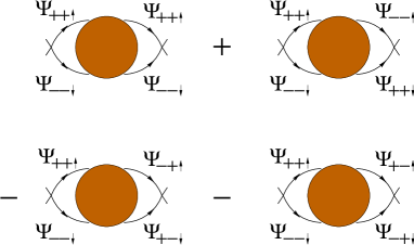
FIG. 13.: Contributions to the response function for $d$-wave pairing, with the same representation as in Fig. 12.

REFERENCES

- [1] A. Yu. Kasumov et al., Science 284, 1508 (1999).
- [2] A. F. Morpurgo et al., Science 286, 263 (1999).
- [3] M. Kociak et al., Phys. Rev. Lett. 86, 2416 (2001).
- [4] L. Balents and M. P. A. Fisher, Phys. Rev. B 55, R11973 (1997).
- [5] Yu. A. Krotov, D.-H. Lee and S. G. Louie, Phys. Rev. Lett. 78, 4245 (1997).
- [6] R. Egger and A. O. Gogolin, Phys. Rev. Lett. 79, 5082 (1997); Eur. Phys. J. B 3, 281 (1998).
- [7] C. Kane, L. Balents and M. P. A. Fisher, Phys. Rev. Lett. 79, 5086 (1997).
- [8] J. W. G. Wildöer et al., Nature 391, 59 (1998). T. W. Odom et al., Nature 391, 62 (1998).
- [9] J. W. Mintmire, B. I. Dunlap and C. T. White, Phys. Rev. Lett. 68, 631 (1992). N. Hamada, S. Sawada and A. Oshiyama, Phys. Rev. Lett. 68, 1579 (1992). R. Saito et al., Appl. Phys. Lett. 60, 2204 (1992).
- [10] V. J. Emery, in Highly Conducting One-Dimensional Solids, ed. J. T. Devreese, R. P. Evrard and V. E. Van Doren (Plenum, New York, 1979).
- [11] J. Sólyom, Adv. Phys. 28, 201 (1979).
- [12] F. D. M. Haldane, J. Phys. C 14, 2585 (1981).
- [13] H. J. Schulz, in Correlated Electron Systems, Vol. 9, ed. V. J. Emery (World Scientific, Singapore, 1993).
- [14] M. Bockrath et al., Nature 397, 598 (1999).
- [15] Z. Yao et al., Nature 402, 273 (1999).
- [16] J. González, Phys. Rev. Lett. 87, 136401 (2001).
- [17] J. González, Phys. Rev. Lett. 88, 076403 (2002).
- [18] Z. K. Tang et al., Science 292, 2462 (2001).
- [19] J. González, F. Guinea and M. A. H. Vozmediano, Nucl. Phys. B 406, 771 (1993).
- [20] R. Egger and H. Grabert, Phys. Rev. Lett. 79, 3463 (1997). S. Bellucci and J. González, Eur. Phys. J. B 18, 3 (2000).
- [21] D. W. Wang, A. J. Millis and S. Das Sarma, Phys. Rev. B 64, 193 307 (2001).
- [22] D. Loss and T. Martin, Phys. Rev. B 50, 12160 (1994).
- [23] R. A. Jishi, M. S. Dresselhaus and G. Dresselhaus, Phys. Rev. B 48, 11385 (1993).
- [24] A. A. Maarouf, C. L. Kane and E. J. Mele, Phys. Rev. B 61, 11156 (2000).
- [25] See also A. Sédéki, L. G. Caron and C. Bourbonnais, report cond-mat/0111296.
- [26] A phase of this kind has been also found in Ref. [22] in the study of the 1D electron system coupled to acoustic phonons.
- [27] This is the case of the superconducting ropes of Ref. [3], although to meet such experimental condition one has to find the appropriate sample out of a large number of them.
- [28] L. Pietronero, S. Strässler, H. R. Zeller and M. J. Rice, Phys. Rev. B 22, 904 (1980).