Passive Random Walkers and River-like Networks on Growing Surfaces

Abstract

Passive random walker dynamics is introduced on a growing surface. The walker is designed to drift upward or downward and then follow specific topological features, such as hill tops or valley bottoms, of the fluctuating surface. The passive random walker can thus be used to directly explore scaling properties of otherwise somewhat hidden topological features. For example, the walker allows us to directly measure the dynamical exponent of the underlying growth dynamics. We use the Kardar-Parisi-Zhang(KPZ) type surface growth as an example. The word lines of a set of merging passive walkers show nontrivial coalescence behaviors and display the river-like network structures of surface ridges in space-time. In other dynamics, like Edwards-Wilkinson growth, this does not happen. The passive random walkers in KPZ-type surface growth are closely related to the shock waves in the noiseless Burgers equation. We also briefly discuss their relations to the passive scalar dynamics in turbulence.

I Introduction

The research on fluctuations of surfaces during growth has been one of the major areas of study in nonequilibrium statistical mechanics in recent decades. Most research is focused on identifying universality classes and the scaling behavior of surface morphology, e.g., how the width of surfaces scales with the size of surfaces Kardar et al. (1986); Kim and Kosterlitz (89); Halpin-Healy and Zhang (1995); Lässig (1998); Kotrla et al. (1998); Chin and den Nijs (1999). Recently, the coupling between surface growth and other degrees of freedom has been considered in the context of ordering phenomena on growing and fluctuating surfaces. For example, the field coupled to the surface can be different species of deposited particlesKotrla et al. (1998); Kotrla and Predota (1997); Drossel and Kardar (2000) or surface reconstruction order parametersChin and den Nijs (2001). Unlike equilibrium surfaces, where the coupling between the surface height degrees of freedom and the additional field is irrelevant at large length scalesden Nijs (1985), we found that the coupling between the surface and the reconstruction orders can not be ignoredChin and den Nijs (2001). The surface and the additional field are usually coupled topologically. For example, the domain walls of order parameters become trapped at the hilltops or in the valleys on surfaces in 1+1 D systemKotrla et al. (1998); Kotrla and Predota (1997); Drossel and Kardar (2000) or on the ridge lines on surfaces in a 2+1 D systemChin and den Nijs (2001).

The fluctuations of the additional degrees of freedom (expressed by the dynamics of the “domain walls”) thus become slaved to the fluctuations of the surface. From the surface perspective, the additional field is usually irrelevant and passive. Therefore, part of the dynamics of the surface and its topological features can be evaluated from the fluctuations of such domain walls that are pinned or trapped to them. We can put probes on the surface to follow these features dynamically. In this paper, passive random walkers(PRWs) are designed to follow hilltops or valley bottoms on the surface.

One of the first applications of the PRWs is to provide a direct way to measure the dynamical exponent of the surface fluctuations. We will also present the phenomena of coalescence of passive random walkers on Kardar-Parisi-Zhang(KPZ)Kardar et al. (1986); Kim and Kosterlitz (89) type growth. The coalescence of passive random walkers uncovers a river-like network structure of the surface in space-time.

Our passive random walkers are similar to the passive scalars in turbulence. This is not surprising because the KPZ equation is equivalent to Burgers equation, which describes a fluidKardar et al. (1986) with different random stirring forces from those in related turbulence studies. It is instructive to study the dynamics of the PRWs from both perspectives.

This paper is organized as follows. The passive random walkers model is defined in Sec.II. The application to directly measuring the dynamical exponent is presented in Sec.III. Then we discuss the coalescence of the PRWs in Sec.IV. The sign of the coupling between the PRWs and the surface is important for the coalescence phenomena as discussed in Sec.VI. In Sec. VII, we show the river-like network in the space-time structure of KPZ-type surfaces and the relation between the passive random walkers and the passive scalars in turbulence is briefly discussed. Other possible applications of the PRW model are pointed out, together with a summary of the results in Sec.VIII.

II Passive Random Walkers on a Growing Surface

We couple a PRW to the growth dynamics of a fluctuating surface. The movement of the PRW is determined by the local slope of the growing surface. The well-known Kim-Kosterlitz (KK) modelKim and Kosterlitz (89) for surface growth is used as an example. In the KK model, a surface is specified by integer height variables on a square lattice. A single particle is deposited at a randomly chosen site $i$ if the restricted solid-on-solid condition ($|\delta h_{ij}|=|h_{j}-h_{i}|\leq 1$ for all nearest neighbor pairs $\langle ij\rangle$) remains satisfied, otherwise, the deposition of the particle is rejected. The surface grows and the stationary state is rough. The position of the PRW is updated after $N_{\rm s}^{2}/v_{\rm g}$ Monte Carlo steps (with $v_{\rm g}$ the growth velocity and $N_{\rm s}$ the total number of site), i.e., when on average one layer of surface material is added, according to the following rules. Let $i$ be the position of the walker. If there is any neighbor site $j$ for which $h_{j}>h_{i}$, then we move the walker to site $j$. If there is more than one site higher than site $i$, then we let the PRW move to either one with equal probability. We apply periodic boundary conditions for both the surface and the PRW motion.

It is known that the continuum limit of the KK model is governed by the so-called KPZ equationKim and Kosterlitz (89),

$$\frac{\partial h}{\partial t}=\nu\frac{\partial^{2}h}{\partial{\bf x}^{2}}+\lambda\left(\frac{\partial h}{\partial{\bf x}}\right)^{2}+\eta_{\rm s},$$ (1)

with uncorrelated noise,

$$\langle\eta_{\rm s}({\bf x},t)\eta_{\rm s}({\bf x}^{\prime},t^{\prime})\rangle=D\delta({\bf x},{\bf x}^{\prime})\delta(t,t^{\prime}).$$ (2)

In the same limit. the equation of motion of the PRW is

$$\frac{\partial u}{\partial t}=\kappa\frac{\partial}{\partial{\bf x}}h({\bf x},t)|_{{\bf x}={\bf u}(t)},$$ (3)

where ${\bf u}(t)$ is the coordinate of the PRW at time $t$, and $\kappa$ is the coupling strength between the PRW and the surface. In our lattice model, $\kappa$ is of the same order as $\lambda$. The equations of motion, Eqs.(1)-(3), imply that the PRW moves upwards for $\kappa>0$. The PRW becomes trapped on a local maximum of the surface profile as seen in Fig.(1) for positive $\kappa$. Once the PRW is trapped on a hilltop, it follows the motion of the hilltop, which is subject to the surface fluctuations. When $\kappa$ is negative, the PRW moves downwards instead of upwards, and the PRW becomes trapped in a valley bottom instead of a hilltop. The relative sign between $\kappa$ and $\lambda$ affects the dynamics of the PRWs. We will focus on positive $\kappa$ for now, and discuss negative $\kappa$ in Sec.VI.

Figure 1: Passive walkers trapped on local hilltops and global maximum in 1+1 D simulations. The dashed lines are the world lines of two PRWs and the solid lines are the surface profiles during growth. The passive walkers follow the local maximums initially and ultimately merge into each other. The walkers reach the global maximum at a later time.

III Dynamical Exponent of Passive Random Walkers

One important observation of the dynamics of an upwards moving PRW on KPZ-type surfaces is that the PRW not only reaches a local maximum in a relatively short time, but also that in finite-size systems it ultimately ends up trapped at the global maximum. We will discuss the detailed mechanism of this phenomenon later in Sec.IV. Once the PRW is trapped on the global maximum, it performs a correlated random walk following the global surface fluctuations. The surface fluctuates critically and is self-affine. Namely, the profile of the surface is invariant under the following rescaling,

$$x\rightarrow b^{-1}x,\,\,h\rightarrow b^{-\alpha}h,\,\,t\rightarrow b^{-1/z_{\rm s}}t,$$ (4)

where $b$ is a scaling factor, $\alpha$ is the roughness exponent, and $z_{\rm s}$ is the dynamical exponent of the surface. The PRW is slaved to the fluctuations of the interface, therefore we expect similar dynamical scaling for the world line of the PRW.

The displacement of the PRW, $\Delta{\bf u}(t)={\bf u}(t)-{\bf u}(0)$, should be defined carefully to avoid confusion in finite-size systems with periodic boundary conditions, where the PRW moves on a ring in 1D and on a torus in 2D. In such manifolds, the winding number of the PRW should be taken into account. The component of the displacement, $\Delta{\bf u}(t)$, in direction ${\rm\hat{e}_{i}}$ is defined as $\Delta u_{\rm\hat{e}_{i}}(t)=n^{+}_{\rm\hat{e}_{i}}-n^{-}_{\rm\hat{e}_{i}}$, with the actual number of right moves, $n^{+}_{\rm\hat{e}_{i}}$, and the actual number of left moves, $n^{-}_{\rm\hat{e}_{i}}$ in direction $\hat{e}_{i}$.

In our numerical simulations, we let the system evolve until both the surface and the PRW motion reach stationary states. Then the value of the displacement $\Delta{\bf u}(t)$ is measured as $\Delta u(t)=\left(\sum_{\rm i}\left(n^{+}_{\rm\hat{e}_{i}}-n^{-}_{\rm\hat{e}_{i}}\right)^{2}\right)^{1/2}$. To accelerate the simulation, we also adopt a rejection-free algorithm. Details of this algorithm can be found in ref.Chin and den Nijs (2001). In this algorithm, time is counted in terms of the numbers of layers of particles deposited instead of the conventional Monte Carlo time unit. We established earlier that the unit of time in this rejection free algorithm is linearly proportional to the Monte Carlo time unitChin and den Nijs (2001)(see also Drossel and Kardar (2000)).

If the PRW indeed is slaved to follow the global surface fluctuations, which are invariant statistically under the transformation eq.(4), the average distance of the displacement, $\Delta u(t)$, must obey the scaling form,

$$\langle\Delta u(t)\rangle\sim L^{\chi}{\cal G}\left(\frac{t}{L^{z_{\rm s}}}\right),$$ (5)

where ${\cal G}(\tau)$ is a universal scaling function. When $t\ll L^{z_{\rm s}}$, the hopping events of the PRW are correlated due to the surface fluctuations, and $\Delta u(t)\sim t^{z_{\rm w}}$, where $z_{\rm w}$ is the dynamical exponent for the PRW. At time scales $t\gg L^{z_{\rm s}}$, the surface fluctuations are limited by the finite size of the lattice and the PRW becomes like a free uncorrelated random walker. Thus, the scaling function ${\cal G}(\tau)$ has the asymptotic forms, ${\cal G}(\tau)\rightarrow\tau^{1/z_{\rm w}}$ for $\tau\ll 1$ and ${\cal G}(\tau)\rightarrow\tau^{1/2}$ for $\tau\gg 1$. The value of the exponent $\chi$ in Eq.(5) follows from the fact that $u(t)$ must be independent of $L$ in the thermal dynamics limit. Consequently, $\chi$, $z_{\rm w}$, and $z_{\rm s}$ are not independent and satisfy the relation $\chi=\frac{z_{\rm s}}{z_{\rm w}}$.

The dynamical exponent of the walker is not necessarily the same as the dynamical exponent of the surface. There is no a priori reason for $\chi=1$, i.e., for $z_{\rm w}=z_{\rm s}$. The numerical results (Fig. 2) indicate that $z_{\rm w}=z_{\rm s}$, but why? $\chi=1$ reflects that there is no length scale other than the system size $L$ involved in the dynamics of the PRW. This is in contrast to free uncorrelated random walks, in which case another length scale proportional to $t^{1/2}$ will emerge. The absence of a new independent length scale is consistent with our picture that the PRW is typically trapped on a global maximum, hence the fluctuations of the PRW follow the dynamical scaling of the surface.

The main numerical results are shown in Fig.(2)-(4). They are obtained by averaging over about $10^{5}$ samples in 1+1D and $4\times 10^{5}$ samples in 2+1D. The displacements of the PRW are determined up to $t=256$ in 1+1D and $t=128$ in 2+1D. In 1+1D, $\langle\Delta u\rangle$ is in the order of $10^{2}$ lattice units at $t=256$. In 2+1D, $\langle\Delta u\rangle\sim 10$ at $t=128$. Although $\langle\Delta u\rangle$ is relatively small in 2+1D, the scaling behaviors are already clear. Small displacements reflect merely a small prefactor in the scaling form eq.(5). This is analogous to a small diffusion constant (which slows the diffusive process, but does not affect the scaling properties even at small spatial scales). Moreover, the asymptotic region of interest is at small $\tau$ and at small $\Delta u/L$, so the scaling behaviors that we focus on are in the small $\Delta u$ interval. By increasing system sizes, we can extend the scaling region of the scaling variable, $\Delta u/L$, about two decades.

We check the scaling form eq.(5) by collapsing the data (see Fig.(2)) with $z_{\rm s}=1.5$ in 1+1 D and $z_{\rm s}=1.6$ in 2+1 D. The prediction, $\chi=1$, gives excellent data collapse, except for the nonuniversal part around $\Delta u\lesssim 10$ in 1+1D and $\Delta u\lesssim 4$ in 2+1D. This nonuniversal behavior is likely caused by the discrete lattice spacing. A more detailed fit of the dynamical exponent $z_{\rm w}$ must avoid this small $\Delta u$ region while keeping $\Delta u/L$ small. In Fig.(3b)(4b), we fit $z_{\rm w}$ by omitting the data from $\Delta u\lesssim 10$ in 1+1D and $\Delta u\lesssim 4$ in 2+1D. It might appear that by ignoring data from these regions, a large fraction of information in the data is lost. In fact, only less than a quarter of the data points fall in these regions. The crossover from uncorrelated random walker behavior ($z=2$, at large $\Delta u/L$) to correlated behavior($z\not=2$, at small $\Delta u/L$) is visible in Fig.(3b)(4b), where the exponent decreases from 2 to $z_{\rm s}$ as the system size increases. We conclude that $z_{\rm w}=1.50(1)$ in the 1+1D and $z_{\rm w}=1.60(1)$ in the 2+1D KK model.

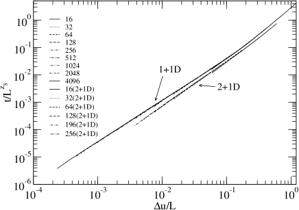
Figure 2: Collapses of $t$ versus $\Delta u$. We use $z_{\rm s}=1.5$ for 1+1D, $z_{\rm s}=1.6$ for 2+1D and $\chi=1$ for both cases.

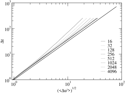
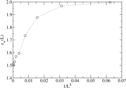
Figure 3: (a)The log-log plot of $t$ versus $\Delta u$ in the 1+1D KK model. For reference, we plot the solid line with a slope of 1.5. (b)Fitting of $z_{\rm w}$ for different system sizes in 1+1D. It shows the crossover from free uncorrelated random walker behavior ($z=2$) to a KPZ-type PRW behavior ($z=1.5$). The dotted line is a convenience to guide the eyes.

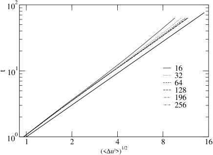
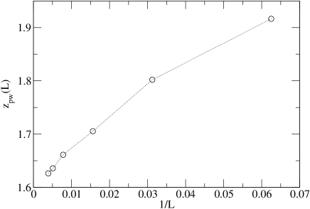
Figure 4: (a)The log-log plot of $t$ versus $\Delta u$ in the 2+1D KK model. For reference, we plot the solid line with a slope of 1.6. (b)Fitting of $z_{\rm w}$ for different system sizes in 2+1D. It shows the crossover from free uncorrelated random walker behavior ($z=2$) to a KPZ-type PRW behavior ($z=1.6$). The dotted line is a convenience to guide the eyes.

Our measurement of $z_{\rm w}$ provides one of the very few independent and direct measurements of the dynamical exponent $z_{\rm s}$ on stationary-state KPZ-type surfaces. Conventional approaches determine the dynamical exponent indirectly, through the measurement of the scaling behaviors of the width of surfaces in the transient states, starting with a flat initial condition. The surface width defined as $W=\langle(h-{\bar{h}})^{2}\rangle^{1/2}$ scales as $W\sim t^{\beta}$ for $t\ll L^{z_{\rm s}}$. Then the dynamical exponent is found by using the scaling relation $z_{\rm s}=\alpha/\beta$. The other method is to measure the correlation function $g(x,t)=\langle\left(h(x_{0}+\Delta x,t_{0}+\Delta t)-h(x_{0},t_{0})\right)^{2}\rangle\sim(\Delta t)^{2\beta}$ for $\Delta t<(\Delta x)^{z_{\rm s}}$ at stationary states. Both methods obtain the dynamical exponent indirectly through the growth exponent $\beta$. By tracing the path of the PRW, we are able to provide an independent and direct measurement of the dynamical exponent without knowledge about the global width of the surface.

Compared to the conventional methods of measuring the dynamical exponent, we only need to acquire information of the local slopes around the PRW. Thus, it is instructive to understand the connection between the slope-slope correlations along the path of the PRW and the global roughening dynamics of the surface.

The displacement of the PRW and the correlation of the slopes are connected by the fluctuation-dissipation theory. The scaling of the dispersion in the PRW displacement can be evaluated from the slope-slope correlation function along the world line of the PRWBohr and Pikovsky (1993), i.e.,

$$\langle({\bf u}(t)-{\bf u}(0))^{2}\rangle\sim t\int_{0}^{t}d\tau\,\Phi(\tau)\sim t^{1/z_{\rm w}},$$ (6)

with $\Phi(\tau)$,

$$\Phi(\tau)=\left\langle\frac{\partial{\bf u}(\tau)}{\partial t}\frac{\partial{\bf u}(0)}{\partial t}\right\rangle\sim\left\langle\frac{\partial}{\partial x}h({\bf u}(\tau),\tau)\frac{\partial}{\partial x}h({\bf u}(0),0)\right\rangle,$$ (7)

This correlation function $\Phi(\tau)$ is different from the conventional slope-slope correlations, ${\tilde{\Phi}}(r,t)=\langle\partial_{x}h(r,t)\partial_{x}h(0,0)\rangle$, where the correlations are calculated at specific fixed $r$. Instead, we need to evaluate the correlation ${\tilde{\Phi}}(r,t)$ along the correlated path, the world line of the PRW, $r=u(t)$.

The most general scaling form for ${\tilde{\Phi}}(r,t)$ is,

$${\tilde{\Phi}}(r,t)=b^{2\eta}{\tilde{\Phi}}\left(b^{-1}r,b^{-z_{\rm s}}t\right),$$ (8)

where $\eta$ is an exponent yet to be determined. This scaling form is equivalent to

$${\tilde{\Phi}}(r,t)\sim t^{2\eta/z_{\rm s}}F\left(r^{-z_{\rm s}}t\right),$$ (9)

with $F(y)$ a scaling function. Since a path of the PRW is determined by the surface fluctuations, averaging over different paths can be approximated by averaging over different realizations of the surface (like different Monte Carlo runs). $\Phi(\tau)$ is approximately equal to the value of ${\tilde{\Phi}(r,t)}$ at $r=\Delta u(t)\sim t^{1/z_{\rm w}}$. Thus, $\Phi(\tau)$ scales as

$$\Phi(\tau)\sim{\tilde{\Phi}}(\tau^{1/z_{\rm w}},\tau)\sim\tau^{2\eta/z_{\rm s}}F\left(\tau^{1-\chi}\right).$$ (10)

If $\chi\geq 1$, asymptotically, the scaling function behaves as $F\left(\tau^{1-\chi}\right)\sim F(0)+F^{\prime}(0)\tau^{1-\chi}$, which approaches a constant, for $\tau\rightarrow\infty$. Hence the correlation function scales as $\Phi(\tau)\sim\tau^{2\eta/z_{\rm s}}$. Together with Eq. (6), we obtain $2+2\eta/z_{\rm s}=2/z_{\rm w}$. This relation allows us to determine $\eta$, which is the scaling dimension of the slope operator, from the measurement of $z_{\rm w}$. Furthermore, if $\chi=1$, then $\eta=\alpha-1$, provided that the KPZ scaling relation $\alpha+z_{\rm s}=2$ holds. This result, $\eta=\alpha-1$, is consistent with Lässig’s operator production expansion scheme Lässig (1998) and our previous workChin and den Nijs (1999) for KPZ type surfaces. Namely, all slope–slope correlations can be obtained by the naive power counting and the slope operator, $\frac{\partial h}{\partial x}$, scales as $x^{\alpha-1}$.

Our numerical results suggest that $\chi$ is indeed equal to 1 for upwards moving PRWs. In 1+1D, renormalization group(RG) calculations gave ${\tilde{\Phi}}(r,t)\sim t^{-1/z_{\rm s}}F(r^{z}/t)$Forster et al. (1977), so our results imply the value of $z$ is fixed as $z_{\rm w}=z_{\rm s}=3/2$ in 1+1 D. In 2+1 D KPZ-type surface growth, RG calculations indicated that the fixed point is at strong coupling such that analytical results can not be obtained perturbativelyKardar et al. (1986). To author’s knowledge, no analytic result for the scaling from of ${\tilde{\Phi}}(r,t)$ has been obtained for 2+1 D. Our numerical results support $\eta=\alpha-1$ for KPZ-type surfaces.

IV Coalescence of Passive random walkers

Why does an upwards moving PRW typically end up on the global maximum? To further understand the mechanism of this phenomenon, we study the dynamics of multiple PRWs on KPZ-type surfaces. If all upward moving PRWs eventually reach the global maximum on the finite-sized KPZ-type surface, then all of them will converge to the same hilltop even though they start at different positions. This is true only if the PRWs have the property of coalescence, namely two PRWs close to each other merge into each other and move together afterward during the process of moving up to the global maximum.

Although, in the definition of the dynamics of the PRWs, the PRWs always move upward, this simple coupling between the PRW and the surface only guarantees that the PRW reaches a local maximum, not the global one. However, we find that in KPZ dynamics with negative $\lambda$ the upwards moving PRWs coalesce. Two PRWs separated over a distance $r$ at time $t=0$ merge into each other after a typical time period $t\sim r^{z_{\rm w}}$ as shown in Fig.(1) ( see also (8a) ). On the contrary, downwards moving PRWs do not coalesce in $\lambda<0$ KPZ-type dynamics and PRWs do not coalesce in Edwards-Wilkinson(EW) type growth (the $\lambda=0$ point of KPZ equation).

Consider the PRWs sitting on two nearby hilltops that have similar heights. The region between the two hilltops is a small and shallow valley. If both the hilltops and the valley are relatively higher than the other parts of the surface, the valley is likely to be filled up and vanish in a short time. These two hilltops merge and the merging event causes the PRWs to coalesce afterward as shown in Fig.(1). The coalescence of the PRWs is likely caused by merging of two nearby hilltops by filling the valley in between.

This trivial argument seems to imply that PRWs will coalesce for any type of growing surface as long as the PRWs are trapped on hilltops. This is not true. We found that the PRWs on EW type surfaces do not coalesce, although KPZ-type surfaces and the EW-type surfaces have the same stationary state and roughness exponent $\alpha=1/2$ in 1+1 D. The following discussion and the detail analysis in Sec.V show how the nonlinear term, $\lambda\left(\partial_{x}h\right)^{2}$, in the KPZ equation(eq.(1)) affects the phenomenon of coalescence.

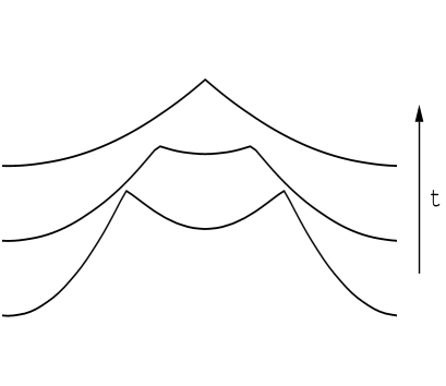
Figure 5: A close look at the coalescence of two hilltops driven by the noiseless KPZ equation. The curves in this figure have been shifted for clarity. The two hilltops have a common contact point at the bottom of the valley between them.

The nonlinear term, $\lambda(\partial_{x}h)^{2}$, in the KPZ equation controls how the growth rate depends on local slopes. Consider a plateau on a surface, for positive $\lambda$, the growth rate on the slope parts of the plateau is larger than the flat top. The flat top of the plateau expands by lateral growth on the slopes. In general, hilltops become flatter than valleys for positive $\lambda$. Negative $\lambda$ has an opposite effect, the slope parts grows slower than the flat tops hence the flat tops become sharper. Shrinking of plateau flat tops is an indication of a negative $\lambda$ in the KPZ equation. The merging events of two hilltops is equivalent to shrinking of flat top plateaus. For example, at larger length scales, the shallow valley between two nearby hilltops and the hilltops themselves as a whole acts like a plateau on the surface (Fig.(5)). Before the coalescence of the hilltops, the size of the flat top of the plateau is the distance between these two hilltops. While these two hilltops are moving towards each other by surface fluctuations, the size of the flat plateau top effectively shrinks, which is an indication of a negative $\lambda$. In the KK model, $\lambda$ is negative and the origin of negative $\lambda$ is due to the restricted solid-on-solid condition $|\Delta h_{ij}|\leq 1$, which reduces the growth rate to zero at the regions where the density of $\Delta h=1$(or $\Delta h=-1$) steps is 1. With negative $\lambda$ for the KK model, which belongs to the KPZ universality class, both the hilltops and the PRWs coalesce.

V Coalescence of Hilltops in the Noiseless KPZ Equation

We can gain insights about the coalescence of the PRWs on KPZ-type surfaces by investigating the solution for the noiseless KPZ equation in the limit $\nu\rightarrow 0$. In that limit, the evolution of surfaces with given initial conditions has an analytical solution, which allows us to study the details of the dynamics of the hilltops.

A detailed derivation of the solution for the noiseless KPZ equation can be found in Woyczyński (1998). We only present a brief review of the derivation. With the Hopf-Cole transformation, $\phi(x,t)=\exp\left(\lambda h(x,t)/\nu\right)$, we can transform the noiseless KPZ equation into a simple linear diffusion equation for $\phi(x,t)$,

$$\frac{\partial\phi}{\partial t}=\nu\frac{\partial^{2}\phi}{\partial x^{2}}.$$ (11)

The solution is a superposition of Gaussian functions weighted by the initial conditions,

$$\phi(x,t)=\left(2\pi\nu t\right)^{-\frac{1}{2}}\int dy\,\phi(y,0)\exp\left(-\frac{(x-y)^{2}}{\nu t}\right),$$ (12)

where $\phi(y,0)=\exp\left(\lambda h(y,0)/\nu\right)$ is the initial condition, determined by the initial height profile $h(y,0)$. In the limit $\nu\rightarrow 0$, we can simplify the solution by introducing the velocity, $v=\partial_{x}h$, as an auxiliary variable,

$$v=\frac{\nu}{\lambda}\frac{\partial\ln\Phi}{\partial x}=\frac{\int dy\,\frac{2(x-y)}{\lambda t}\exp\left(-\frac{1}{\nu}\left(\frac{(x-y)^{2}}{t}+\lambda h(y,0)\right)\right)}{\int dy\exp\left(-\frac{1}{\nu}\left(\frac{(x-y)^{2}}{t}+\lambda h(y,0)\right)\right)}.$$ (13)

By the method of steepest descent in the limit $\nu\rightarrow 0$, this yields

$$v(x,t)=\frac{-2(x-y_{\rm min}(x,t))}{\lambda t},$$ (14)

where $y_{\rm min}$ is a function of both $x$ and $t$, and it is determined by taking $y$ where $\frac{(x-y)^{2}}{t}-\lambda h(y,0)$ is a minimum for fixed $x$ and fixed $t$. Namely,

$$y_{\rm min}(x,t)=\arg\min_{y}\left(\frac{(x-y)^{2}}{t}-\lambda h(y,0)\right).$$ (15)

The $y_{\rm min}(x,t)$ are usually only piecewise continuous functions of $x$, particularly for random initial conditions generated by random walkers. Shock waves of the velocity field are formed where $y_{\rm min}(x,t)$ is discontinuous.

Assuming $y_{\rm min}(x,t)$ is constant between $x$ and $y_{\rm min}$, we can further integrate $v(x,t)$:

$$h(x,t)=\frac{-(x-y_{\rm min}(x,t))^{2}}{\lambda t}+c_{\rm h},$$ (16)

where $c_{\rm h}$ is the integration constant. The solution for $h(x,t)$ is reduced to the problem of finding $y_{\rm min}$ and $c_{\rm h}$.

Determining $y_{\rm min}$ for $\lambda<0$ is equivalent to finding $y$ for which the vertical distance is the shortest between the initial height configuration, $h(y,0)$, and the parabola, $\frac{(x-y)^{2}}{\lambda t}$, centered at $x$, while the parabola is approaching the surface from below. $y_{\rm min}$ is the first contact point between the two curves $h(y,0)$ and $\Psi(y;x,t)=\frac{(x-y)^{2}}{\lambda t}+c$ while $c$ is adjusted to $c(x,t)=h(y_{\rm min},0)-\frac{(x-y_{\rm min})^{2}}{\lambda t}$ (Fig.(6)). The contact point $y_{\rm min}$ is where $h(y,0)-\frac{(x-y)^{2}}{\lambda t}$ is a minimum. Once $y_{\rm min}$ is found, $h(x,t)$ follows from eq.(16) with $c_{\rm h}=h(y_{\rm min},t)$. Thus, we have $h(x,t)=\Psi(x;x,t)=c(x,t)$, which is the top of the parabola. The surface between $x$ and $y_{\rm min}(x,t)$ is also parabolic in shape at time $t$. It is possible that there exists more than one first contact point for certain $x$ and $t$. If this happens, $y_{\rm min}(x,t)$ as a function of $x$ will be discontinuous at that specific $x$.

This solution has an intuitive graphical interpretation, which is useful for understanding the coalescence phenomena. The evolution of the surfaces is generated by a sequence of geometry transformations on the surfaces at an earlier time. For negative $\lambda$, the new surface at time $t$ is obtained by scanning the original surface from below with a probe that has a parabolic shaped tip, $\Psi(y;x,t)=\frac{(x-y)^{2}}{\lambda t}+c(x,t)$(Fig.(6)) for negative $\lambda$. (For positive $\lambda$, the probe scans the surface from above instead.) The probe is centered at position $x$, and $c(x,t)$ (the vertical position of the top of the tip) is adjusted by moving the probe up and down. When the probe approaches the surface from below, it stops when it starts to come into contact with the surface. The horizontal position of the first contact point between the probe and the surface is $y_{\rm min}(x,t)$. Since the probe stops moving upward once it comes in contact with the surface, we might think of the vertical position of the tip of the probe, $c(x,t)$, as the height of the new surface seen by the probe at $x$ at time $t$. The probe scans through the surface and plots a new surface that gives the surface evolved by the noiseless KPZ equation at a later time. Because the parabolic shape of the probe, the new surface usually consists of a collection of parabola shaped segments(the dashed curves shown in Fig.(6)).

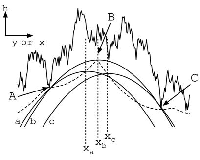
Figure 6: The parabolic shape probe tip scans through point $x_{a}$,$x_{b}$, and $x_{c}$ from left to right. Curves (a),(b),and (c) are parabola which are centered at $x_{a}$, $x_{b}$, and $x_{c}$ respectively. Curve (a)/(b) only contact with the initial random surface at point A/B. Curve (b) contacts with the initial surface at both point A and C. While the probe is scanning through $x_{b}$, the first contact point jumps from A to C. Thus, $y_{\rm min}(x)$ is discontinued at point $x_{b}$ and the path of the tip creates a cusp at point C. The dashed curve is the surface generated by the path of the probe tip.

With this geometrical interpretation of the exact solution of the noiseless KPZ equation, we are able to visualize how the singular hill tops are formed and to discuss the dynamics of coalescence of the hill tops. If the local average curvature over a region such as between A and C in Fig.(6) is larger than the curvature of the tip of the probe at time $t$, then the tip cannot reach the surface everywhere between point A and C. When the probe scans through this region, at point B in Fig.(6), there are two first contact points for the parabola, and $y_{\rm min}(x)$ is discontinued at this point. At points where the function $y_{\rm min}(x)$ is not continuous, the path of the tip forms cusps, which is are hilltops of the new surface. The position of the hilltop in Fig.6 is determined by the positions of the two contact points A, C and the curvature of the probe tip.

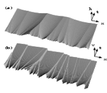
Figure 7: (a)The evolution of the surface under transformation eq.(17). Hilltops coalesce and form tree-like structures. (b) The coalescence of shock waves in the velocity field. The velocity is defined as $v=\frac{\partial h}{\partial x}$.

We can also write the solution of $h(x,t)$ as a functional transformation $\cal T$ defined as

$${\cal T}_{t}(h(x,t_{0}))\equiv h(x,t+t_{0})=\min_{y}\left(h(y,t_{0})-\frac{(x-y)^{2}}{\lambda t}\right).$$ (17)

This transformation has the following property,

$${\cal T}_{t_{1}+t_{2}}(h(x,t_{0}))={\cal T}_{t_{2}}{\cal T}_{t_{1}}(h(x,t_{0})).$$ (18)

The geometrical interpretation of the solution in this form is similar to the Huygens principle growth algorithmTang et al. (1990), except that parabola shaped wave fronts instead of circular or spherical wave fronts are used. The transformation eq.(17) can be applied iteratively and is suitable for evaluating the evolution of surfaces numerically.

We evaluate the evolution of a random initial surface with Eq.(17). The coalescence of the hilltops is shown clearly in Fig.(7a). Why do those hilltops coalesce and how do they move? Will hilltop B in Fig.(6) move towards point A or point C? Answers to these questions can be addressed with the equation of motion of the hilltops.

The curvature of the probe at time $t$ is equal to $1/(\lambda t)$. The probe becomes broader and broader with time. As long as the absolute value of the local curvature around the contact points, A or C, is much larger than the absolute value of the curvature of the probe, the positions of these two contact points do not change. In this case, the height difference $h(x_{\rm A},t)-h(x_{\rm C},t)$, where $x_{\rm A}$ and $x_{\rm C}$ are the horizontal coordinates of points A and C respectively, is also a constant. It can be written as

$$h(x_{\rm A},t)-h(x_{\rm C},t)=$$

$$(h(x_{\rm A},t)-h(x_{\rm B},t))-(h(x_{\rm C},t)-h(x_{\rm B},t)).$$

The curve between A and B and the curve between B and C of the new surface are two parabolas. With $h(x_{\rm A},t)-h(x_{\rm B},t)=(x_{\rm A}-x_{\rm B})^{2}/(\lambda t)$ and $h(x_{\rm C},t)-h(x_{\rm B},t)=(x_{\rm C}-x_{\rm B})^{2}/(\lambda t)$, we obtain the equation of motion of the hilltop,

$$\frac{\partial x_{\rm B}}{\partial t}=t^{-1}\left(x_{\rm B}-\frac{x_{\rm A}+x_{\rm C}}{2}\right).$$ (19)

This equation implies that the hilltops always move toward the closest of the two contact points. Moreover, the closest contact point is also the higher one. If two neighboring hilltops share the same contact point, and that contact point is the highest one for both hilltops, then these two hilltops will merge into one around the position of the shared contact point as illustrated in Fig.(5). A sequence of coalescence events of the hilltops forms a tree-like structure of world lines as in Fig (7a).

The dynamics of the coalescence of the hilltops in the noiseless KPZ equation is totally deterministic and only depends on initial surfaces. In the noisy case, the dynamics becomes stochastic, however, the qualitative behavior of the coalescence of the hilltops is still sustained even when the surface is perturbed with randomly depositions. The nonlinear term causes the coalescence of the hill tops and remains essential even when the dynamics is stochastic. To check that the nonlinear term is responsible for the coalescence in the stochastic dynamics, we apply our upwards moving PRW model to EW-type surfaces. The upwards moving PRWs for EW type surface do not coalesce although the density of the PRWs is slightly higher on the hilltops.

VI downwards moving passive random walkers

So far we have focused only on the case in which $\kappa$ and $\lambda$ have opposite signs, i.e., when the PRWs move upward($\kappa>0$) in the KK model ($\lambda<0$). The discussion in the preceding section suggests that the shape of the surface has very different characteristics between a hilltop and a valley bottom on the surface with noiseless KPZ dynamics. Namely, hilltops are sharp with discontinued slopes while valley bottoms are rounded and with continuous slopes. The symmetry is broken by the nonlinear term. We also found that valley bottoms vanish by themselves, instead of coalescing with others valleys.

If $\kappa$ is negative, the PRWs move toward the valley bottoms. It is interesting to see how the PRWs respond to such qualitative aspects of the surface in the presence of stochastic noise. In the deterministic case, the hilltops and valley bottoms intertwine, the number of valley bottoms and the number of hilltops both decrease. This is not true for the stochastic case. New microscopic hilltops and valley bottoms are being formed constantly by the noisy depositions of particles. Is the coalescence of the PRWs stable under such perturbations? Of upwards moving PRWs in the KK model, coalescences are stable against the noise. As we will see next, the coalescence of the downwards moving PRWs is not stable against random depositions.

Consider the upwards moving PRWs. Suppose noise splits the hilltops by creating a small valley between them. This small valley is unstable against the dynamics as we have seen in the preceding section. These two hilltops will merge again soon as a result of the nonlinear term in the KPZ equation. The nonlinear KPZ dynamics stabilizes the coalescence of the upwards moving PRWs.

Next, imagine several downward moving PRWs moving into the same valley. The aggregation of the PRWs is not stable against the noisy perturbation. Depositions of particles on the valley split the valley. A PRW on the original valley bottom can go to either one of those two valleys with equal probability, so both valleys will be occupied by PRWs. Do the new created subvalleys always merge back into each other? A valley bottom does not move in the noiseless case; they will remain separated by the hilltop. The hilltop does not vanish unless it is driven away to merge with other hilltops, which is a much less likely process than the splitting. Therefore, dynamics like this does not stabilize the aggregation of downwards moving PRWs. They tend to be separated under the growth dynamics and we expect that the dynamics of downwards moving PRWs, trapped in valley bottoms, is dominated by the perturbation of random deposition rather than the deterministic nonlinear term in the dynamics. In Fig.(8c), we show a typical simulation for downwards moving PRWs. Instead of coalescence, we find that the aggregation clusters of PRWs are not stable and split constantly.

Coalescence of the upwards moving PRWs for negative $\lambda$ is an important feature of KPZ-type surfaces. Not only does it ensure that the PRWs end up trapped on the global maximum; it also reveals the space-time structure of KPZ-type surfaces in detail, i.e., hilltops (valley bottoms) coalesce as time evolving for negative (positive) $\lambda$.

Our analysis on the KPZ equation applies to the phenomena of coalescence of the shock waves in the inviscid($\nu\rightarrow 0$) noiseless Burgers equation. The velocity in the Burgers equation is the slope on the KPZ-type surfaces, i.e., $v=\partial_{x}h$. By differentiation of eq. (1), it becomes

$$\frac{\partial v}{\partial t}=\lambda v\cdot\frac{\partial v}{\partial x}+\frac{\partial^{2}v}{\partial x^{2}}+\eta_{\rm B}.$$ (20)

The noise term satisfies $\langle\eta_{\rm B}(x,t)\eta_{\rm B}(0,0)\rangle\sim\partial_{x}^{2}\delta(x)\delta(t)$. Because the slopes of the surface are discontinuous at the hilltops, the hilltops on KPZ-type surfaces correspond to the shock waves in the Burgers equation. The coalescence of the hilltops of the surface indicates that the shock waves coalesce, as illustrated in Fig.(7(b)). Coalescences of shock waves described by the noiseless Burgers equation have been reported in a numerical study of inelastic collisions of particles in 1+1 dimensionsBen-Naim et al. (1999). Bohr and Pikovsky also showed that the zeros in the velocity field of the Burgers equation coalesceBohr and Pikovsky (1993). The above analysis for the coalescence of KPZ hilltops translates directly into the coalescence of shock waves in the Burgers equation with noise. Our analysis on coalescences of PRWs on a growing surface presented here not only provides further intuitive and detailed understanding of the mechanism of these coalescence phenomena but also explains, in both deterministic and stochastic dynamics, the different behaviors between hilltops and valleys, which are distinct types of zeros in the velocity field in the Burgers turbulences.

VII River-like network and Passive Scalars

To further understand the stability of the aggregations of PRWs, we study how random forces, in addition to the driving forces from surface slopes, are applied to the PRWs directly and change the tree-like structure of the PRW world lines in Fig.(8a). Is the tree-like structure stable? Random noise modifies the equation of motion of the PRW as

$$\frac{\partial u}{\partial t}=\kappa\frac{\partial}{\partial x}h(x,t)|_{x=u(t)}+\eta_{\rm w}(x,t),$$ (21)

with $\eta_{\rm w}$ the uncorrelated noise, $\langle\eta_{\rm w}(x,t)\eta_{\rm w}(0,0)\rangle=D_{\rm w}\delta(x)\delta(t)$. $D_{\rm w}$ is the diffusion constant of the PRW if $\kappa=0$.

First consider a single PRW on a surface. The second term on the right hand side of eq.(21) introduces the ordinary diffusive behavior, i.e., $\Delta u(t)\sim(D_{\rm w}t)^{1/2}$. The scaling behavior due to the first term, $\Delta u(t)\sim(K_{\rm w}t)^{1/z_{\rm w}}$, ($K_{\rm w}$ is a constant determined by $\kappa$ and $\lambda$) still dominates the large scale behavior since $1/z_{\rm w}>2$. However, the PRW appears as diffusive instead of super-diffusive at length scales smaller than $l_{\rm c}\sim\left(\frac{D_{\rm w}}{K_{\rm w}}\right)^{\frac{1}{2-z_{\rm w}}}$.

The diffusive noise also affects the coalescence of multiple PRWs. For small perturbations, the aggregation is stable because the PRWs cannot escape from the hilltop by diffusion if the hilltop is high and large enough. The net effect of diffusion simply broadens the coalescence cluster. However, if we increase the strength of the random noise, the PRWs can escape from the hilltop and be caught by other hilltops nearby with finite probability. In this case, the cluster of coalescence PRWs splits and the world lines of the PRWs form a braid-like network instead of a tree structure. A typical configuration of such a braid-like network is shown in Fig.(8b). Both the tree-like and the braid-like network resemble river-like networks of different length scales in NatureRodríguez-Iturbe and Rinaldo (2001).

The crossover scale between tree-like networks and braid-like networks is given by $l_{\rm c}$. We observe diffusive behaviors locally at scales less than $l_{\rm c}$. The braid-like networks emerge at the crossover scale, $l_{\rm c}$, and the tree-like structures are recovered at scales much larger than $l_{\rm c}$.

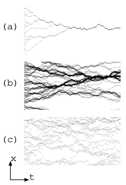
Figure 8: World lines of passive walkers for different parameters. The lines are the paths of 128 PRW on a system of size L=128. The darkness is proportional to the number of PRWs for each site. In (a), the system is simulated in the limit $l_{\rm c}=\left(\frac{D_{\rm pw}}{K}\right)^{\frac{1}{2-z}}\rightarrow 0$ for upward moving PRWs. In (b), we choose $l_{\rm c}\sim L$, the system size. (c) is the result of downwards moving PRWs in the limit $l_{\rm c}\rightarrow 0$. Even without a diffusion term in eq. (21), the downwards moving PRWs do not coalesce. The dynamics of the downwards moving PRWs on KK-type surface is dominated by the uncorrelated random depositions.

Furthermore, we can consider the evolution of the probability distribution function, $P(x,t)$, of finding a particle at position $x$ at time $t$. Note that the total number of PRWs is conserved in our model. Therefore, $P(x,t)$ has the standard conserved form,

$$\frac{\partial P(x,t)}{\partial t}=\nabla\cdot j(x,t),$$ (22)

where $j(x,t)$ is the PRW current. The current is the sum of the advected part and the diffusive contribution, i.e., $j(x,t)=\kappa vP(x,t)+D_{\rm w}\partial_{x}P(x,t)$. Hence, we have

$$\frac{\partial P(x,t)}{\partial t}=\kappa\nabla(vP(x,t))+D_{\rm w}\nabla^{2}P(x,t).$$ (23)

This is simply the equation of motion of passive scalars, $P(x,t)$, in a fluid. In the limit $D_{\rm w}\rightarrow 0$, the passive scalars will be concentrated at a globe hilltop as we have seen in the previous sections if $\kappa$ and $\lambda$ have opposite sign for a finite system.

VIII Concluding remarks

Motivated by the domain wall dynamics on nonequilibrium fluctuating surfaces, we study the dynamics of passive random walkers on KPZ-type growing surfaces. We show that, although the coupling rule between a PRW and a surface is defined locally, the PRW typically reaches the maximum of the surface over a distance $x$ in a time scale $t\sim x^{{\rm z}_{s}}$ and “feels” the fluctuations of the surface over the same length scale. Two PRWs separated by $\Delta x$ coalesce after $\Delta t\sim(\Delta x)^{{\rm z}_{s}}$. The fluctuations of the positions of such PRWs follow the same dynamical scaling as the KPZ fluctuations. We verify this scaling behavior numerically. Tracing the paths of the PRWs on KPZ-type surfaces is an effective method to measure the dynamical exponent directly in the stationary state.

In addition to the scaling, the dynamics of passive random walkers reveals detailed specific space-time structures of a KPZ-type growing surface, i.e., hilltops coalesce with each other and the world lines of the PRWs form self-affine tree-like structures. We provide an analytical argument explaining this phenomenon based on the noiseless Burgers-KPZ equation. We show how the nonlinear term $(\partial_{x}h)^{2}$ is responsible for this nontrivial coalescence phenomenon in both the noiseless and noisy case. The noiseless KPZ equation also allows us to understand why downwards moving PRWs do not coalesce, due to the asymmetry between hilltops and valley bottoms.

We want to emphasize that the effectively attractive interactions which makes the PRWs coalesce are not only topological but also robust against perturbations. For KPZ-type growth, the $(\partial_{x}h)^{2}$ term breaks the symmetry between hilltops and valley bottoms during growth and introduces nontrivial dynamics of the hilltops for negative $\lambda$ and the valley bottoms for positive $\lambda$. The singularities on KPZ-type surfaces generated by the nonlinear terms stabilize the aggregations of the PRWs against other perturbations. The coalescence of PRWs reveals one of the important features of the complicated space-time structure of the surface. An interesting extension of this study is to see how to generalize this to different universality classes of surface dynamics. We already point out that in EW growth, because of the particle-hole symmetry, PRWs do not coalesce. For other nonlinear models, in which the nonlinear terms break up-down symmetry, PRWs may be driven in other nontrivial ways and the surface may show interesting space-time structures.

Depending on the strength of the noise applied to the PRWs, the world lines of PRWs form tree-like or braid-like networks in space-time. The tree-like or the braid-like networks resemble river type networks in nature. The braid-like networks are the result of two competing mechanisms, namely, the coalescence between PRWs caused by the fluctuations of surfaces and the diffusion of PRWs caused by directly applied noise. These two mechanisms define a crossover length scale $l_{\rm c}$, and give rise to the braid-like networks at this scale. One might expect to see similar crossover phenomena in the study of passive scalars in Burgers turbulence.

Previous studies on fluctuating nonequilibrium surfaces were focused on the scaling behavior. This study shows that, beyond global scaling laws, such as the scaling of the global interface width, nonlinear surface growth dynamics leads to intriguing detailed aspects of their space-time structures. We hope studying these different perspectives of nonequilibrium dynamics can lead to a better understanding of these complex systems.

This research is supported by the National Science Foundation under grant No. DMR-9985806. The author thanks Marcel den Nijs for many useful discussions and critical reading of the manuscript.

References

- Kardar et al. (1986) M. Kardar, G. Parisi, and Y.-C. Zhang, Phys. Rev. Lett. 56, 889 (1986).
- Kim and Kosterlitz (89) J. M. Kim and J. M. Kosterlitz, Phys. Rev. Lett. 62, 2289 (89).
- Halpin-Healy and Zhang (1995) T. Halpin-Healy and Y.-C. Zhang, Physics Reports 254, 215 (1995).
- Lässig (1998) M. Lässig, Phys. Rev. Lett. 80, 2366 (1998).
- Kotrla et al. (1998) M. Kotrla, F. Slanina, and M. Pr̈edota, Phys. Rev. B 58, 10003 (1998).
- Chin and den Nijs (1999) C. S. Chin and den Nijs, Phys. Rev. E 59, 2633 (1999).
- Kotrla and Predota (1997) M. Kotrla and M. Predota, Europhys. Lett. 39, 251 (1997).
- Drossel and Kardar (2000) B. Drossel and M. Kardar, Phys. Rev. Lett. 85, 614 (2000).
- Chin and den Nijs (2001) C. S. Chin and den Nijs, Phys. Rev. E 64, 031606 (2001).
- den Nijs (1985) M. den Nijs, J. Phys. A 18, L549 (1985).
- Bohr and Pikovsky (1993) T. Bohr and A. Pikovsky, Phys. Rev. Lett. 70, 2892 (1993).
- Forster et al. (1977) D. Forster, D. R. Nelson, and M. J. Stephen, Phys. Rev. A 16, 732 (1977).
- Woyczyński (1998) W. A. Woyczyński, Burgers-KPZ Turbulence (Springer, 1998).
- Tang et al. (1990) C. Tang, S. Alexander, and R. Bruinsma, Phys. Rev. L 64, 772 (1990).
- Ben-Naim et al. (1999) E. Ben-Naim, S. Y. Chen, G. D. Doolen, and S. Redner, Phys. Rev. Lett. 83, 4069 (1999).
- Rodríguez-Iturbe and Rinaldo (2001) I. Rodríguez-Iturbe and A. Rinaldo, Fractal River Basins (Cambridge University Press, 2001).