Effective Heisenberg-Model Description of the Coupled Spin-Pseudospin Model
for Quarter-Filled Ladders

Abstract

Quantum Monte Carlo method is used to study the coupled spin-pseudospin Hamiltonian in one-dimension (1D) that models the charge-ordering instability of the anisotropic Hubbard ladder at quarter filling. We calculate the temperature dependence of the uniform spin susceptibility and the spin and charge excitation spectra of the system to show that there is a parameter and temperature region where the spin degrees of freedom behave like a 1D antiferromagnetic Heisenberg model. Anomalous spin dynamics in the disorder phase of a typical charge-ordered material $\alpha^{\prime}$-NaV₂O₅ is thereby considered.

1 Introduction

Charge-ordering (CO) instability has recently been one of the major topics in the field of strongly correlated electron systems. Here, elucidation of the observed anomalous behaviors of electrons associated with the CO phase transition has been the central issue. This includes questions on the charge dynamics above the transition temperature $T_{\rm CO}$ as well as on the CO spatial patterns realized below $T_{\rm CO}$. A well-known example is the vanadate bronze $\alpha^{\prime}$-NaV₂O₅ where the system may be modeled as a lattice of coupled ladders (or a trellis lattice) at quarter filling.[1, 2, 3, 5, 4] Strong intersite Coulomb interaction between electrons is believed to be the origin of the CO instability.[2, 3] In this material, the CO with a zigzag ordering pattern is observed below $T_{\rm CO}=34$ K,[6, 7, 8, 9, 10] and associated with this, a number of anomalous behaviors, which can be related to the slow dynamics of charge carriers (or charge fluctuation), have been observed above $T_{\rm CO}$.[11, 12, 13, 14, 10, 15, 16, 17] Anomalous response of the spin degrees of freedom has also been noticed.[18, 9, 19] It seems therefore quite natural to wonder how in such systems the spin degrees of freedom behave near the CO phase transition when they are on the slowly fluctuating charge carriers. In this paper, we thus consider the issue: what are the consequences of charge fluctuation at $T>T_{\rm CO}$ to the spin degrees of freedom?

One of the simplest models that allow for such situation is the anisotropic Hubbard ladders at quarter filling with the strong intersite Coulomb repulsion. We here use an effective Hamiltonian written in terms of the spin and pseudospin (representing charge degrees of freedom) operators.[5, 20, 21, 17] This Hamiltonian is derived from the Hubbard ladder model by the perturbation theory[5, 20, 21] where the hopping parameter between the rungs of the ladder is assumed to be small compared with the onsite and intersite Coulomb repulsions as well as the hopping parameter in the rung (i.e., the anisotropic ladder).[3] Although the CO is not realized in this model (since it is the 1D quantum-spin model), we can simulate anomalous behaviors of the spin degrees of freedom under the strong charge fluctuation. We will apply the quantum Monte Carlo (QMC) method to this model to calculate the temperature dependence of the uniform spin susceptibility and the spin and charge excitation spectra, thereby clarifying consequences of the interplay between its spin and charge degrees of freedom.

We note that, in this coupled spin-pseudospin model, the spin exchange interaction is necessarily associated with the charge excitation; i.e., the spin excitations cannot occur without making the exchange of the pseudospins. We will then show that nevertheless there is a parameter and temperature region where the spin degrees of freedom behave like a 1D antiferromagnetic Heisenberg model; i.e., the spin degrees of freedom are ‘separated’ from the charge degrees of freedom in this region. We will moreover show that the spin system behaves in different manner depending on whether the temperature $T$ is below or above a crossover temperature $T^{*}$ which is related to the pseudospin excitations; at $T\lesssim T^{*}$, it behaves like a 1D antiferromagnetic Heisenberg model with a $T$-independent effective exchange coupling constant $J_{\rm eff}$ with large renormalization, whereas at $T\gtrsim T^{*}$, $J_{\rm eff}$ decreases rapidly with increasing $T$, where the effective Heisenberg-model description ceases to be valid.

This paper is organized as follows. In §2, we define the coupled spin-pseudospin model that describes the spin and charge degrees of freedom of the anisotropic Hubbard ladder at quarter filling. Some details of the method of calculation are also given. In §3, we present the results of calculation which include the staggered susceptibility for pseudospins, the spin and pseudospin excitation spectra, and the temperature dependence of the uniform spin susceptibility. Discussion on the experimental relevance to $\alpha^{\prime}$-NaV₂O₅ and summary of the paper will be given in §4.

2 Model and Method

Our effective spin-pseudospin Hamiltonian may be written as a sum

$${\cal H}={\cal H}_{0}+{\cal H}_{\rm ST}$$ (1)

of the quantum Ising Hamiltonian for pseudospins

$${\cal H}_{0}=J_{1}\big{(}-\frac{g}{2}\sum_{i}T_{i}^{x}+\sum_{i}T_{i}^{z}T_{i+1}^{z}\big{)}$$ (2)

and the spin-pseudospin coupling term

$${\cal H}_{\rm ST}=J_{2}\sum_{i}\big{(}{\bf S}_{i}\cdot{\bf S}_{i+1}-\frac{1}{4}\big{)}\big{(}T_{i}^{+}T_{i+1}^{-}+{\rm H.c.}\big{)}.$$ (3)

The standard notation is used here. ${\bf S}_{i}$ and ${\bf T}_{i}$ are, respectively, the spin and pseudospin operators of spin-1/2 at site $i$, where $T_{i}^{z}=-1/2$ ($+1/2)$ means the electron is on the left (right) site on the rung of the ladder. $J_{1}$ is the energy scale of the pseudospin system and $J_{2}$ is the coupling strength between the spin and pseudospin systems.

From the second-order perturbation theory,[5, 20, 21] we have the relations $J_{1}=2V_{\parallel}$ and $J_{2}=4t_{\parallel}^{2}/V_{\perp}$, where $t_{\parallel}$ and $V_{\parallel}$ ($t_{\perp}$ and $V_{\perp}$) are the nearest-neighbor hopping parameter and Coulomb repulsion of the leg (rung) of the ladder, respectively. We should then have $J_{1}>J_{2}$, which we assume throughout the present work. We also assume the onsite Coulomb repulsion to be $U\rightarrow\infty$. Relative strength of the transverse field to the pseudospins is measured by $g=4t_{\perp}/J_{1}=2t_{\perp}/V_{\parallel}$. Note that $g$ in the quantum Ising model represents the relative strength of the fluctuation of a charge in the rung: if we assume one electron in a rung, we have the prefactor $gJ_{1}/2$ in the first term of eq. (2), which is the difference between the energies of the bonding and antibonding levels of the rung, $2t_{\perp}$. Thus, if $g$ (or $t_{\perp}$) is large the electron is stable in the bonding level of the rung, but if $g$ (or $t_{\perp}$) is small the effect of $V_{\parallel}$ easily leads the system to CO.

We use the conventional world-line QMC method for the analysis of the model. We use a 32-site cluster (where a site contains a spin and a pseudospin) with periodic boundary condition; the cluster-size dependence of the calculated results are examined by using clusters up to 96 sites but we find no significant size dependence in the results. Because the model does not conserve the total pseudospin, we have examined a number of ways of the spin flips and confirmed that available analytical results are reproduced correctly.[22] The maximum-entropy method is used to calculate the dynamical quantities like the spin and pseudospin excitation spectra.

3 Calculated Results

3.1 Staggered susceptibility for pseudospins

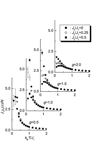
Figure 1: Temperature dependence of the staggered susceptibility for pseudospins $\chi_{\rm T}(\pi)$ calculated for the coupled spin-pseudospin Hamiltonian.

The response function is defined as

$$\chi_{ij}=\int_{0}^{\beta}\!{\rm d}\lambda\,\big{(}\langle S_{j}^{z}(-i\lambda)S_{i}^{z}\rangle-\langle S_{j}^{z}\rangle\langle S_{i}^{z}\rangle\big{)}$$ (4)

where $S_{j}^{z}(-i\lambda)$ is the Heisenberg representation of $S_{j}^{z}$ and $\langle\cdots\rangle$ is the canonical average. $\chi_{ij}$ is Fourier transformed to the $q$-dependent susceptibility $\chi(q)$, which we calculate by the QMC method; the $q\rightarrow 0$ limit gives the uniform spin susceptibility $\chi(T)$ and the staggered susceptibility is defined as $\chi(q)$ at $q=\pi$. In the following, we use the subscripts ${\rm S}$ and ${\rm T}$ as in $\chi_{\rm S}(q)$ and $\chi_{\rm T}(q)$, which stand for the spin and pseudospin degrees of freedom, respectively.

The phase diagram of the quantum Ising model ${\cal H}_{0}$ is well known;[23] at $T=0$ there is a long-range order for $g<1$ ($g=1$ is a quantum critical point), which corresponds to the zigzag (or ‘antiferromagnetic’) CO. The calculated staggered susceptibility for pseudospins is shown in Fig. 1, where we find that it shows divergent behavior at $T\rightarrow 0$ for $g<1$. The dispersion relation of the pseudospin excitation observed in the calculated dynamical structure factor (shown in Fig. 2, see below) agrees well with the exact result:[23]

$$\omega_{q}=\frac{J_{1}}{2}\sqrt{1+g^{2}+2g\cos q}.$$ (5)

We find in Fig. 1 that the inclusion of the coupling term ${\cal H}_{\rm ST}$, which introduces the quantum fluctuation via the factor $T_{i}^{+}T_{j}^{-}$, suppresses the divergence. Thus, we may say that the inclusion of the spin degrees of freedom in the quantum Ising model for pseudospins leads to the unstable long-range CO.

3.2 Spin and pseudospin excitation spectra

[t]

Dynamical pseudospin structure factor $S_{\rm T}(q,\omega)$ for the coupled spin-pseudospin model calculated at $k_{\rm B}T=0.1J_{2}$. The results at $J_{2}/J_{1}=0$ are for the quantum Ising model. The peak at $\omega=0$ for $J_{2}/J_{1}>0$ in the uppermost panel of (a) and (b) is spurious, which is due to the error of the maximum entropy method.

[t]

Dynamical spin structure factor $S_{\rm S}(q,\omega)$ for the coupled spin-pseudospin model calculated at $k_{\rm B}T=0.1J_{2}$.

The dynamical pseudospin structure factor $S_{\rm T}(q,\omega)$ is defined as

$$S_{\rm T}(q,\tau)=\frac{1}{N}\sum_{r_{1},r_{2}}e^{-iq(r_{2}-r_{1})}\langle T_{r_{1}}^{z}(\tau)T_{r_{2}}^{z}(0)\rangle$$ (6)

$$S_{\rm T}(q,\tau)=\frac{1}{\pi}\int_{0}^{\infty}\!{\rm d}\omega\,S_{\rm T}(q,\omega)K(\omega,\tau)$$ (7)

$$K(\omega,\tau)=e^{-\omega\tau}+e^{-\omega(\beta-\tau)}$$ (8)

where $S_{\rm T}(q,\tau)$ is the Fourier transform of the imaginary-time correlation function. We use the maximum entropy method for the inverse Laplace transformation (or analytical continuation) to obtain $S_{\rm T}(q,\omega)$ from $S_{\rm T}(q,\tau)$. The dynamical spin structure factor $S_{\rm S}(q,\omega)$ is similarly defined by replacing the pseudospin operator $T^{z}_{r}$ with the spin operator $S^{z}_{r}$.

The calculated results for the pseudospin excitation spectra at low temperature ($k_{\rm B}T=0.1J_{2}$) are shown in Fig. 2, where we find that the spectra are under strong influence of the spin-pseudospin coupling term $J_{2}$. With increasing the coupling strength $J_{2}/J_{1}$, the peak of the pseudospin spectra shifts to higher energies and simultaneously the spectra are broadened. Thus, the lower-energy edge of the peak is not affected strongly by the coupling strength $J_{2}$, at least when $g$ is large. It seems reasonable to suppose that the scattering of the pseudospin excitations due to spin excitations causes the broadening of the spectra.

The calculated results for the spin excitation spectra at low temperature are shown in Fig. 3, where we find that, in contrast to the pseudospin spectra, the spin excitation spectra change very little; i.e., the peak position, width, as well as the shape of the spectra are not affected by the parameter $J_{1}$ when $g\gtrsim 1$. When $g$ is small, however, the peak position is slightly shifted to lower energies with increasing the value of $J_{1}$ (see Fig. 3 (a)).

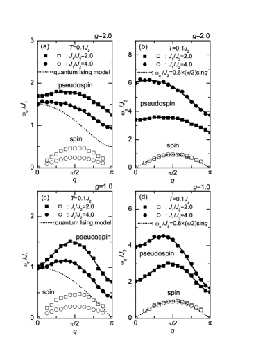
Figure 2: Dispersion relations of the spin (open symbols) and pseudospin (solid symbols) excitations calculated at $k_{\rm B}T=0.1J_{2}$. Note that the same data at $g=2$ (at $g=1$) are plotted in (a) and (b) (in (c) and (d)) in different energy scales $J_{1}$ and $J_{2}$. The dotted line in (a) and (c) is the dispersion relation for the quantum Ising model eq. (5), and that in (b) and (d) is the scaled dispersion relation for the 1D antiferromagnetic Heisenberg model eq. (9).

The dispersion relation of the spin and pseudospin excitations calculated at low temperature are summarized in Fig. 4, which are obtained as the momentum dependence of the peak position of the spectra. For comparison, we show the dispersion of the quantum Ising model in Fig. 3 (a) and (c); the gap opens when $g>1$, which is closed at $q=\pi$ when $g\rightarrow 1$, leading to the ‘antiferromagnetic’ long-range order (or zigzag CO). We note that the gap remains open irrespective of the value of $g$ when we include the coupling term $J_{2}$. In Fig. 4, we present the same dispersion relations in a different energy scales, i.e., $\omega_{q}/J_{1}$ and $\omega_{q}/J_{2}$. We find that, unless $g$ is small, the spin excitation spectra are always inside the charge gap, i.e., inside the gap of the pseudospin excitation spectrum; when the charge gap is large, the energy scale of the spin excitations is separated from the high-energy charge excitations. With decreasing $g$, however, the energy of the charge excitation decreases at the momentum $q=\pi$ to couple with the spin excitations. We find in Fig. 4 (b) and (d) that for $g\gtrsim 1$ the dispersion of the spin excitation spectra scales very well with $J_{2}$; i.e., it does not depend on the value of $J_{1}$. The dispersion of the calculated spin excitation spectra is fitted well with the dispersion of the 1D antiferromagnetic Heisenberg model

$$\omega_{q}/J_{2}=0.6\times\frac{\pi}{2}\sin q$$ (9)

if we include the factor $0.6$ as in eq. (9). The factor is independent of $J_{1}$ for $g\gtrsim 1$ and at low $T$.

These results suggest that at low temperatures there is a parameter region where the spin degrees of freedom behaves independently from the pseudospin degrees of freedom; it is when $g\gtrsim 1$ and the gap of the pseudospin excitation spectra is large, inside of which there is a spin excitation spectra. Thus, we suggest the validity of the decoupling of the coupling term of the Hamiltonian as

$${\cal H}_{\rm ST}\Rightarrow J_{2}\sum_{i}\big{<}T_{i}^{+}T_{i+1}^{-}+{\rm H.c.}\big{>}\big{(}{\bf S}_{i}\cdot{\bf S}_{i+1}-\frac{1}{4}\big{)}$$ (10)

with

$$\big{<}T_{i}^{+}T_{i+1}^{-}+{\rm H.c.}\big{>}\simeq 0.6$$ (11)

which leads to the effective Heisenberg-model description of the spin degrees of freedom of our model.

3.3 Uniform spin susceptibility

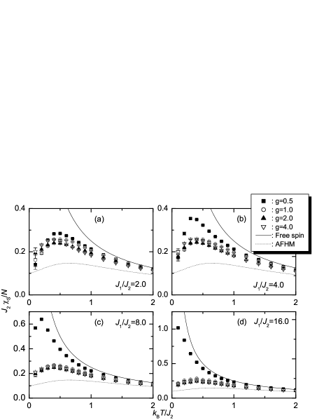
Figure 3: Temperature dependence of the uniform spin susceptibility $\chi_{\rm S}$ calculated for the coupled spin-pseudospin Hamiltonian. The solid and dotted curves are the uniform susceptibility for the system of noninteracting $S=1/2$ spins and that for the 1D antiferromagnetic Heisenberg model, respectively.

To see the validity of the effective Heisenberg-model description further, in particular for its temperature dependence, we calculate the temperature dependence of the uniform spin susceptibility for the coupled spin-pseudospin Hamiltonian. The results are shown in Fig. 5, where comparisons are made with the uniform susceptibility for the system of free spins and with that for the 1D antiferromagnetic Heisenberg model. We find that the temperature $k_{\rm B}T/J_{2}$ at which $J_{2}\chi_{\rm S}(T)$ shows a maximum is lower than that of the 1D antiferromagnetic Heisenberg model; it becomes lower with decreasing the value of $g$ or with increasing the value of $J_{1}/J_{2}$. In other words, the deviation from the Heisenberg model is large when the quantum fluctuation of the pseudospins is small, which occurs when $g$ is small or $J_{1}$ is large.

Now, let us analyze the data more precisely. In order to do this, we fit the results with the temperature dependence of the spin susceptibility of the 1D antiferromagnetic Heisenberg model, the so-called Bonner-Fisher curve;[24] i.e., we introduce the $T$-dependent effective exchange coupling constant $J_{\rm eff}(T)$ and we determine the values so as to fit the calculated uniform spin susceptibility $\chi_{\rm S}(T)$. If the values of $J_{\rm eff}$ thus obtained do not depend on $T$, it follows that the spin degrees freedom of our spin-pseudospin model is reduced to a 1D Heisenberg model

$${\cal H}_{\rm spin}=J_{\rm eff}\sum_{i}\big{(}{\bf S}_{i}\cdot{\bf S}_{i+1}-\frac{1}{4}\big{)}$$ (12)

at least for the response to the uniform magnetic field. The results are shown in Fig. 6. We find that the estimated value of $J_{\rm eff}(T)$ is indeed a constant for temperatures below $k_{\rm B}T\lesssim 0.7J_{2}$ at $g=2$. A crossover temperature $T^{*}$ $(=0.7J_{2})$ is thereby defined. The effective exchange coupling constant takes a value

$$J_{\rm eff}\simeq 0.6J_{2}$$ (13)

which is consistent with the value estimated from the dispersion relation of the spin excitation spectra (see §3.2). We find that also at $g=4$ the scaling behavior holds up to a higher temperature ($k_{\rm B}T\lesssim 0.8J_{2}$), but with the same value of $J_{\rm eff}$ (see Fig. 6 (d)), demonstrating the validity of the effective Heisenberg-model description at $T>T^{*}$. At $g=1$, however, the temperature region where $J_{\rm eff}(T)$ takes a constant value is already very small, although the value is still $J_{\rm eff}\sim 0.6J_{2}$ at $T\sim 0$ K, and at $g=0.5$, the value of $J_{\rm eff}$ at $T\sim 0$ K deviates largely from $J_{\rm eff}=0.6J_{2}$ (or decreases strongly when $J_{1}/J_{2}$ is large), where the effective Heisenberg-model description completely fails.

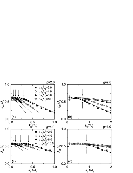
Figure 4: Effective exchange coupling constant $J_{\rm eff}(T)$ estimated from the fitting of the calculated uniform spin susceptibility to the Bonner-Fisher curve.[24] Note that the same data are plotted as a function of $k_{\rm B}T/J_{1}$ (left panels) and of $k_{\rm B}T/J_{2}$ (right panels), whereby a scaling behavior is seen in the latter. The arrows indicate the crossover temperature $T^{*}$. The solid lines are the guide to the eye.

We note here that the crossover temperature $T^{*}$ roughly scales with $J_{2}$ rather than $J_{1}$, as seen in Fig. 6. One might suppose that it should scale with the size of the charge gap: i.e., up to temperatures corresponding to the energy of the lowest charge excitations, with which the pseudospins can excite, the spin excitations may be written in terms of the 1D antiferromagnetic Heisenberg model. However, as we have discussed in §3.2, the size of the charge gap shows a rather complicated behavior and does not simply scale with either $J_{2}$ or $J_{1}$. The naive picture thus does not hold. It may be said however that, since there is no other excitations available, the deviation from the 1D Heisenberg-model description is necessarily due to the pseudospin excitations.

4 Summary and Discussion

We have calculated the spin and pseudospin excitation spectra and the temperature dependence of the uniform spin susceptibility of the coupled spin-pseudospin Hamiltonian by using the QMC method. We have first shown that, when the pseudospin quantum fluctuation is large ($g\gtrsim 1$), the dispersion relation of the spin exitation spectra of our model at low temperatures agrees well with that of the 1D antiferromagnetic Heisenberg model with the renormalized effective exchange coupling constant $J_{\rm eff}=0.6J_{2}$ that is independent of the energy scale of the pseudospin system $J_{1}$. Here, the spin excitation spectra is well inside the charge gap, and thus the spin degrees of freedom are separated from the charge degrees of freedom. We then have shown that the temperature dependence of the uniform spin susceptibility of our model is well described again by the 1D antiferromagnetic Heisenberg model with the same effective exchange coupling constant $J_{\rm eff}=0.6J_{2}$. The description is valid up to the crossover temperature $T^{*}$ that is related to the pseudospin excitations of the system and roughly scales with $J_{2}$ unless the quantum fluctuation of the pseudospins is small ($g\lesssim 1$). We have thus demonstrated the validity of the effective Heisenberg-model description of the coupled spin-pseudospin model for the quarter-filled ladders. It then follows that the coupling between the spin and pseudospin degrees of freedom, which occurs at $g\lesssim 1$, leads to the anomalous spin and charge dynamics of the system.

Although the real material $\alpha^{\prime}$-NaV₂O₅ is modeled well as a 2D trellis-lattice system rather than a 1D ladder system and thus we need great caution in the direct application of the present results, it may be interesting to have a rough idea of the values of the physical parameters appropriate for $\alpha^{\prime}$-NaV₂O₅; according to ref. [3], we have $t_{\parallel}\sim 0.14$ eV, $t_{\perp}\sim 0.30$ eV, and $V_{\parallel}\sim V_{\perp}\sim 0.8$ eV, which lead to $J_{1}\sim 1.6$ eV, $J_{2}\sim 0.10$ eV, and $g\sim 0.75$. Thus, the real material may be in the region of $g\lesssim 1$, where the spin degrees of freedom are not separated from the charge degrees of freedom. The anomalous response of the spin degrees of freedom may therefore be expected. We would here point out, e.g., that the value of $J_{\rm eff}$ estimated from the uniform susceptibility observed in experiment (which takes the value $\sim 600-700$ K at $T\sim 0$ K) decreases with increasing temperature,[9] which is consistent with the results of our calculation. The reported[19] anomalous temperature dependence of the nuclear spin-lattice relaxation rate $1/T_{1}$ is also interesting in this respect. To clarify the dynamics of the spin-charge coupled systems near the real CO phase transition, we however need not only to examine the region $g\lesssim 1$ in greater detail but also to include the 2D coupling in the present model, which we want to leave for future study.

Because the anomalous charge dynamics has been noticed also in other transition-metal oxides[25] and some organic systems[26], we hope that the present study will stimulate further researches on the intriguing interplay between the spin and charge degrees of freedom of strongly correlated electron systems with CO instability.

References

- [1] H. Smolinski, C. Gros, W. Weber, U. Pechert, G. Roth, M. Weiden, C. Geibel: Phys. Rev. Lett. 80 (1998) 5146.
- [2] H. Seo and H. Fukuyama: J. Phys. Soc. Jpn. 67 (1998) 2602.
- [3] S. Nishimoto and Y. Ohta: J. Phys. Soc. Jpn. 67 (1998) 2996.
- [4] P. Thalmeier and P. Fulde: Europhys. Lett. 44 (1998) 242.
- [5] M. V. Mostovoy and D. I. Khomskii: Solid State Commun. 113 (2000) 159.
- [6] M. Isobe and Y. Ueda: J. Phys. Soc. Jpn. 65 (1996) 1178.
- [7] T. Ohama, H. Yasuoka, M. Isobe, and Y. Ueda: Phys. Rev. B 59 (1999) 3299.
- [8] H. Sawa, E. Ninomiya, T. Ohama, H. Nakao, K. Ohwada, Y. Murakami, Y. Fujii, Y. Noda, M. Isobe, and Y. Ueda: J. Phys. Soc. Jpn. 71 (2002) 385.
- [9] D. C. Johnston, R. K. Kremer, M. Troyer, X. Wang, A. Klümper, S. L. Bud’ko, A. F. Panchula, and P. C. Canfield: Phys. Rev. B 61 (2000) 9558.
- [10] For a review, see T. Ohama: Bussei Kenkyu (Kyoto) 74 (2000) 391 [in Japanese].
- [11] S. Ravy, J. Jegoudez, and A. Revcolevschi: Phys. Rev. B 59 (1999) R681.
- [12] H. Nakao, K. Ohwada, N. Takesue, Y. Fujii, M. Isobe, and Y. Ueda: Physica B 21-243 (1998) 534.
- [13] A. Damascelli, C. Presura, D. van der Marel, J. Jegoudez, and A. Revcolevschi: Phys. Rev. B 61 (2000) 2535.
- [14] C. Presura, D. van der Marel, A. Damascelli, and R. K. Kremer: Phys. Rev. B 61 (2000) 15762.
- [15] S. Nishimoto and Y. Ohta: J. Phys. Soc. Jpn. 67 (1998) 3679.
- [16] S. Nishimoto and Y. Ohta: J. Phys. Soc. Jpn. 67 (1998) 4010.
- [17] M. V. Mostovoy, J. Knoester, and D. I. Khomskii: Phys. Rev. B 65 (2002) 064412.
- [18] J. Hemberger, M. Lohmann, M. Nicklas, A. Loidl, M. Klemm, G. Obermeier, and S. Horn: Europhys. Lett. 42 (1998) 661.
- [19] T. Ohama et al.: unpublished.
- [20] M. Cuoco, P. Horsch, and F. Mack: Phys. Rev. B 60 (1999) R8438.
- [21] D. Sa and C. Gros: Eur. Phys. J. B 18 (2000) 421.
- [22] For details, see T. Nakaegawa: Master thesis (Chiba University, 2002).
- [23] S. Sachdev: Quantum Phase Transitions (University Press, Cambridge, 1999).
- [24] J. C. Bonner and M. E. Fisher: Phys. Rev. 135 (1964) A640.
- [25] R. Amasaki, Y. Shibata, and Y. Ohta: cond-mat/0110333.
- [26] Y. Shibata, S. Nishimoto, and Y. Ohta: Phys. Rev. B 64 (2001) 235107.