Chapter 1 Renormalization Group Technique for Quasi-one-dimensional Interacting Fermion Systems at Finite Temperature

C. Bourbonnais, B. Guay and R. Wortis

Abstract

We review some aspects of the renormalization group method for interacting fermions. Special emphasis is placed on the application of scaling theory to quasi-one-dimensional systems at non zero temperature. We begin by introducing the scaling ansatz for purely one-dimensional fermion systems and its extension when interchain coupling and dimensionality crossovers are present at finite temperature. Next, we review the application of the renormalization group technique to the one-dimensional electron gas model and clarify some peculiarities of the method at the two-loop level. The influence of interchain coupling is then included and results for the crossover phenomenology and the multiplicity of characteristic energy scales are summarized. The emergence of the Kohn-Luttinger mechanism in quasi-one-dimensional electronic structures is discussed for both superconducting and density-wave channels.

Contents

toc

1 Introduction

Scaling ideas have exerted a far-reaching influence on our understanding of complex many-body systems. Their use in the study of critical phenomena has offered a broad and fertile field of work at the heart of which is the Wilson formulation of the renormalization group method. [1, 2] In the Wilson view, fluctuations of the order parameter at all length scales up to the correlation length are the key ingredient in explaining the existence of power law singularities that govern critical properties in accordance with scaling laws. Equally powerful is the extension of scaling concepts to anisotropic systems, namely when small anisotropic parameters are magnified as a result of their coupling to singular fluctuations. Intermediate length scales thus emerge giving rise to changes or crossovers in the critical behavior.[3, 4, 5] The horizon of applications of this methodology was further widened when scaling was applied to quantum critical systems for which quantum mechanics governs fluctuations of the order parameter at the critical point.[6, 7]

There has been a parallel expansion of the use of scaling tools in the description of many-fermion systems. This was especially true for the Kondo impurity and the one-dimensional fermion gas problems. In the latter, the reduction of spatial dimension is well known to enlarge the range of fluctuations which have a peculiar impact on the properties of the system.[8, 9] In this context the scaling theory commonly termed multiplicative renormalization group,[10, 11] contributed significantly to the completion of a coherent microscopic picture of the 1D fermion gas system as a paradigm of a non Fermi $-$ Luttinger $-$ liquid state. However, this scaling theory rests for the most part upon the logarithmic structure of infrared singularities that compose 1D perturbation theory and as such departs somewhat from the standard Wilson picture. It remains closer to earlier formulations of the renormalization group in quantum field theory. Yet, fluctuations that characterize the 1D fermion gas do show a multiplicity of length scales stretching from the shortest distance, of the order of the lattice constant, up to the quantum coherence length or the de Broglie wavelength of fermions. Early attempts to reexamine the properties of low dimensional fermion gas system along these lines were motivated by the coupled chains problem,[12, 13, 14, 15, 16] which finds concrete applications in the physics of quasi-one-dimensional organic conductors. [17, 18] The description of interacting fermions when strong spatial anisotropy is present shares many traits with its counterpart in critical phenomena.[5, 4] Hence the Wilson method provides a powerful framework to study how deviations from perfect 1D scaling are introduced by spatial anisotropy. The corresponding length scales enter as key components of the notoriously complex description of dimensionality crossovers in which the 1D state evolves either towards the emergence of a Fermi liquid or the formation of long-range order at finite temperature.

The Wilson renormalization group approach has attracted increasing interest in several areas of the many-fermion problem,[19] notably in the description of two-dimensional systems in connection with high-T_c materials,[20, 21, 22] Fermi liquids,[23, 24, 25] and ladder systems.[26, 27, 28] Within the bounds of this review, it would therefore be impossible to give anything more than a cursory account of the expanding literature in this field[29, 30, 31]. With the goal of keeping this paper self-contained for the non-specialist, however, our interest will be more selective and will focus on the application of the renormalization group to the quasi-one-dimensional fermion gas at finite temperature.[32] Although many aspects of this problem have already been discussed in detail in previous reviews,[15, 16] it is useful to revisit some issues while in addition discussing features of the Wilson method that deserve closer examination but which have as yet never received a detailed investigation. This is especially true in regard to the formulation of the method itself, in particular the way successive integrations over fermion states in outer momentum shells (the Kadanoff transformation) is carried out when high order calculations are performed. We close this review by a detailed discussion of the dual nature of the Kohn-Luttinger mechanism[33] from which interchain pairing correlations find their origin in quasi-one-dimensional systems.[34, 35, 36, 37] With the aid of the renormalization group,[38, 39] we show how this mechanism may yield instabilities of the metallic state towards either unconventional superconducting or density-wave order.

In section II, we introduce scaling notions for fermions in low dimension from a phenomenological standpoint and predictions of the scaling hypothesis are compared to the solution in the non-interacting case in section III. The formulation of the renormalization group in the classical Wilson scheme is given in section IV and explicit calculations are carried out up to the two-loop level. In section V, the influence of interchain coupling is discussed and we go through various possibilities of dimensionality crossovers in the quasi-one-dimensional Fermi gas. In section VI, we study how the Kohn-Luttinger mechanism for interchain pairing correlation emerges from the renormalization group flow and under what conditions it can lead to long-range order. We conclude in section VII.

2 Scaling ansatz for fermions

Before embarking on the program sketched above, it is first useful to discuss on purely phenomenological grounds how scaling notions apply to 1D and quasi-1D fermion systems. The predictions of the scaling ansatz are explicitly checked in the trivial but instructive case of the non-interacting Fermi gas.

2.1 One dimension

Let us look at how scaling ideas apply to the description of purely one-dimensional fermionic systems at low temperature. The temperature $T$ is the parameter that controls the quantum delocalization or the spatial coherence of each particle in one dimension. This appears as a characteristic length scale, $\xi$, which is precisely the de Broglie wavelength. The temperature dependence of $\xi$ is readily determined by considering the effect of thermal excitations on fermion states within an energy shell $\delta\epsilon(k)\sim T$ ($k_{B}\equiv 1,\hbar\equiv 1$), where $\epsilon(k)$ is the energy spectrum of fermions evaluated with respect to the Fermi level. In the vicinity of the Fermi points $\pm k_{F}$, one has $\delta\epsilon(k)\approx v_{F}(\mid k\mid-\ k_{F})$, where $v_{F}$ is the Fermi velocity, and the coherence length can be written

$$\xi\sim v_{F}/T\sim T^{-\nu},$$ (1.1)

where the exponent $\nu$ is then equal to unity. As $T\to 0$, $\xi$ goes to infinity and the system develops long-range quantum coherence. The ‘time’ $\tau$ required for quantum delocalization up to $\xi$ is therefore $\sim 1/T$ which simply implies that

$$\tau\sim\xi^{z}.$$ (1.2)

where $z=1$ is the dynamical exponent of the fermion field. Since ‘time’ and distance must be considered on the same footing, both $\nu$ and $z$ can be taken as independent of interaction.

Let us now consider the Matsubara-Fourier transform

$$G(k,\omega_{n})=\int_{0}^{\beta}\!\!\!\int_{0}^{L}e^{-ikx\,+\,i\omega_{n}\tau}\,G(x,\tau)\,dxd\tau,$$ (1.3)

where

$$G(x,\tau)=-\,\langle T_{\tau}\,\psi_{\alpha}(x,\tau)\psi_{\alpha}^{\dagger}(0,0)\rangle$$ (1.4)

is the one-particle time-ordered correlation function expressed as a statistical average over fermion fields $\psi_{\alpha}^{(\dagger)}$ of spin $\alpha$. Here $\omega_{n}=(2n+1)\pi T$ corresponds to the Matsubara frequencies. For non interacting fermions and $T=0$, $G(k)\sim(\mid k\mid-\ k_{F})^{-1}$ has a simple pole singularity at $|k|\to k_{F}$ and $\omega_{n}=0$, indicating that single particle excitations are well defined. However, when fermions interact in one dimension, such a picture is expected to be altered. In the scaling picture, this can be illustrated by adding an anomalous power dependence on the wave vector near $k_{F}$, namely

$$G(k)\sim(\mid k\mid-\ k_{F})^{-1+\theta}.$$ (1.5)

The absence of a quasi-particle pole introduces $\theta$, the anomalous dimension for the Green’s function ($\theta\geq 0$ where the equality occurs in the non-interacting limit). Correspondingly, the absence of a Fermi liquid component at zero temperature will affect the equal-time decay of coherence at large distance, which takes the form

$$G(x)\approx{\hat{C}\over x^{\bar{d}-1+\theta}},$$ (1.6)

where the effective dimension $\bar{d}=2$ has a space and time component. A similar decay in time takes place for large $\tau$ at $x=0$. Looking at the temperature dependence of the Green’s function, the scaling hypothesis allows us to write

$$G(k,\omega_{n})\approx CT^{-\bar{\!\gamma}}g\big{(}\delta k\,\xi,\omega_{n}\,\xi^{z}\big{)},$$ (1.7)

where $\delta k=|k|-k_{F}$, $\bar{\!\gamma}$ is the thermal exponent of the single particle Green’s function, and $g(x,y)$ is a scaling function. Consistency between Eqns. (1.7) and (1.5) leads to the following relation between the exponents

$$\bar{\!\gamma}=(1-\theta)\nu.$$ (1.8)

Scaling can also be applied to the free energy per unit length, the temperature dependence of which can be expressed as

$$f=-{T\over L}\ln Z\approx AT^{1-\alpha}.$$ (1.9)

The exponent $\alpha$ is connected to the temperature variation of specific heat

$$C_{L}= -T{\partial^{2}f\over\partial T^{2}}$$ (1.10)

$$\approx A^{\prime}T^{-\alpha},$$ (1.11)

where

$$\alpha=1-\bar{d}\nu.$$ (1.12)

As long as the ansatz $\nu=1$ holds for the coherence length, one then always has $\alpha=-1$ in one spatial dimension. The specific heat is therefore linear in temperature for fermions even though, according to Eqn. (1.5), the system is no longer a Fermi liquid at low energy. It should be noted that the familiar Sommerfeld result $C_{V}\sim T$ for a Fermi liquid (and Fermi gas) in higher dimensions indicates that the importance put on fermion states near the Fermi level one-dimensionalizes the sum over states for the evaluation of internal energy.

Scaling concepts can also be applied to the critical behavior of correlations that involve pairs of fermions in one dimension. Superconducting and $2k_{F}$ density-wave responses are among the pair susceptibilities that may present singularities at zero temperature. Consider the Matsubara-Fourier transform of the susceptibility

$$\chi(q,\omega_{m})=\int_{0}^{\beta}\!\!\!\int_{0}^{L}\,e^{-iqx+i\omega_{m}\tau}\chi(x,\tau)\,dxd\tau,$$ (1.13)

where $\omega_{m}=2m\pi T$. The time-ordered pair correlation function is

$$\chi(x,\tau)=-\langle T_{\tau}O(x,\tau)O^{\dagger}(0,0)\rangle,$$ (1.14)

in which $O^{\dagger}\sim\psi^{\dagger}_{\alpha}\psi^{\dagger}_{\beta}$ ($O^{\dagger}\sim\psi_{\alpha}^{\dagger}\psi_{\beta}$) are the composite operators of the superconducting (density-wave) channel, commonly called the Cooper (Peierls) channel. At $T=0$, these can show long-range coherence leading to an algebraic decay of pair correlations with distance. Following the example of the correlation of the order parameter at a critical point, one can write a relation of the form

$$\chi(x)\approx e^{iq_{0}x}{D\over x^{\bar{d}-2+\eta}}~{},$$ (1.15)

where $\eta\geq 0$ is an anomalous exponent that characterizes the decay of pair correlation. Here $q_{0}=0\ (2k_{F})$ is the characteristic wave vector of correlations in the Cooper (Peierls) channel. A similar power law variation with time $\tau$ can also be written at small distance. Correspondingly, in Fourier space, one has in the static limit

$$\chi(q)\approx{\bar{D}\over q^{2-\eta}}~{},$$ (1.16)

where $q$ refers to deviations with respect to an ordering wave vector $q_{0}$ in the Cooper or Peierls channel. For $q=0$ and at finite frequency, a similar expression holds with $q$ being replaced by the frequency. Now at finite temperature, the scaling hypothesis allows us to write

$$\chi(x,T)\approx De^{iq_{0}x}x^{-\bar{d}+2-\eta}{\cal X}(x/\xi),$$ (1.17)

where ${\cal X}$ is scaling function (${\cal X}(0)=1$ ). Here the correlation length $\xi$ for the pair field is assumed to have the same power law dependence on temperature as the coherence length Eqn. (1.1) for both fermions in a pair. In Fourier space, one can write for the divergence of the susceptibility in a given channel

$$\chi(q,\omega_{m},T)\approx\bar{D}T^{-\gamma}\bar{\cal X}(q\xi,\omega_{m}\xi^{z}).$$ (1.18)

Consistency between Eqns. (1.18) and (1.16) in the static case leads to the Fisher relation

$$\gamma=(2-\eta)\nu$$ (1.19)

between the exponents of the static susceptibility, the correlation function and the correlation length.

2.2 Anisotropic scaling and crossover phenomena

Let us now move from one-dimensional systems to quasi-one- dimensional systems by which we mean weakly coupled chains. A dimensionality crossover in low dimensional fermion systems is induced by a small coupling between chains. The nature of this crossover will depend on the kind of coupling involved. Weakly coupled chains correspond to so-called quasi-one-dimensional anisotropy, a situation realized in practice for electronic materials such as the organic conductors,[17, 18, 40] lattice of spin chains, etc. In ordinary critical phenomena, scaling concepts were extended to anisotropic systems and have been successful in describing the new length scales introduced by anisotropy; [3, 4, 5] their use in the study of anisotropic fermion systems appears therefore quite natural. For example, deconfinement of quantum coherence for single particles can give rise to the restoration of a Fermi liquid component below some characteristic low energy scale. In addition, the deconfinement of pair correlations in more than one spatial dimension can lead to the emergence of true long-range order at finite temperature.[41]

Let us consider first the case of interchain single-particle hopping (Fig. 1), whose amplitude $t_{\perp}$ is small compared to the Fermi energy of isolated chains ($t_{\perp}\ll E_{F}$). Applying the extended scaling ansatz to the single fermion Green’s function at $\mid k\mid=k_{F}$, and $\omega_{n=0}=\pi T$,[4] one can write

$$G(T,k_{\perp})\approx DT^{-\bar{\gamma}}X_{G}(Bt_{\perp}(k_{\perp})/T^{\phi_{x}}).$$ (1.20)

$t_{\perp}(k_{\perp})=t_{\perp}\cos k_{\perp}$ and $k_{\perp}$ is the transverse momentum of the Fermion spectrum (here the inter-chain distance $d_{\perp}$ has been set equal to unity). $\phi_{x}>0$ is the crossover exponent which governs the magnification of the single-particle perturbation $t_{\perp}$ as $\xi$ increases along the chains (Fig. 1). $X_{G}(y)$ is called a crossover scaling function and it determines transitory aspects of the crossover and the temperature range over which it is achieved. Here $X_{G}(0)=1$. When $y\ll 1$, the coherence of the fermionic system is confined along the chains and the physics is essentially dominated by the one-dimensional expression (1.7). Otherwise for $y\gg 1$, a different temperature dependence is expected to arise. The temperature scale for the single-particle crossover is thus determined by the condition $y\sim 1$, that is

$$T_{x}\sim t_{\perp}^{1/\phi_{x}}.$$ (1.21)

Well below $T_{x}$ and on the full Fermi surface ${\bf k}={\bf k}_{F}$, one has

$$G(T)\sim z(t_{\perp})T^{-\dot{\bar{\gamma}}},$$ (1.22)

where $z(t_{\perp})$ is the quasi-particle weight and $\dot{\bar{\gamma}}=1$ is the Fermi liquid exponent that restores the canonical dimension of the Green’s function. In order to match (1.20) and (1.22) well below $T_{x}$, one must have [4]

$$z(t_{\perp})=z_{\infty}\ t_{\perp}^{-(\bar{\gamma}-\,\dot{\bar{\gamma}})/\phi_{x}},$$ (1.23)

where $z_{\infty}$ is a non universal constant. Applying scaling to the dynamical $-$ coherent $-$ part of the single-particle Green’s function, the recovery of Fermi liquid behavior yields

$$G({\bf k},\omega_{n})\approx{z(t_{\perp})\over[i\omega_{n}-E({\bf k})]^{\dot{\bar{\gamma}}}}\$$ (1.24)

with $\dot{\bar{\gamma}}=1$ again.

FIGURE 1: One-fermion interchain hopping. $\xi$ is the fermion coherence length along the chains.

Interchain coupling will affect the temperature dependence of pair correlations as well, which can undergo a dimensionality crossover and in turn an instability towards the formation of long-range order either in the Cooper or the Peierls channel at finite temperature. This possibility is of course bound to the number of components of the order parameter and the spatial dimensionality of the system.[41] The scaling behavior of pair correlations is therefore analogous to the one found in ordinary anisotropic critical phenomena. Properties of the system close to the true critical point at $T_{c}$ can then be described by the usual reduced temperature

$$\dot{t}={T-T_{c}\over T_{c}}.$$ (1.25)

The static pair susceptibility at some ordering wave vector ${\bf Q}_{0}\equiv(q_{0},q_{\perp 0})$ will then diverge as $\dot{t}\to 0$ according to

$$\chi(T)\approx\dot{C}(g_{\perp})\,\dot{t}^{-\dot{\!\gamma}},$$ (1.26)

where $\,\dot{\!\gamma}$ is the susceptibility exponent.

Applying the extended scaling hypothesis to the static susceptibility in the superconducting or the density-wave channel, one can write

$$\chi(T)\approx\bar{D}T^{-\gamma}X(Bg_{\perp}/T^{\phi_{x^{2}}}),$$ (1.27)

where $X(y)$ is a crossover scaling function $(X(0)=1)$, $g_{\perp}$ is the inter-chain coupling for pairs of fermions and $\phi_{x^{2}}$ is a two-particle crossover exponent.[15, 42] Following the same arguments as in the single-particle case, the change in the exponents will occur when $y\sim 1$, which allows us to introduce the crossover temperature for pair correlations

$$T_{x^{2}}\sim g_{\perp}^{1/\phi_{x^{2}}}.$$ (1.28)

It is worth noting that the interchain coupling $g_{\perp}$ for pairs of particles differs from $t_{\perp}$, and the two-particle crossover can occur above its single particle counterpart $T_{x}$, in which case the restoration of Fermi liquid behavior is absent. Instead only pair correlations deconfine, possibly leading to long-range order.

If the scaling hypothesis holds, the expressions (1.26) and (1.15) have to match near $T_{c}$, which implies

$$\dot{C}(g_{\perp})=C_{\infty}\ g_{\perp}^{-(\gamma-\dot{\gamma})/\phi_{x^{2}}},$$ (1.29)

where $C_{\infty}$ is a non universal constant. Another prediction of the scaling hypothesis concerns the shift in $T_{c}$ from zero temperature[4]

$$T_{c}(g_{\perp})\sim T_{x}\sim g_{\perp}^{1/\phi_{x^{2}}}$$ (1.30)

When the system undergoes its two-particle dimensionality crossover, the temperature dependence of singularities near $T_{c}$ is governed by the correlation length

$$\dot{\vec{\!\xi}}=\,\dot{\vec{\!\xi}}_{0}\ \dot{\!t}^{-\dot{\nu}},$$ (1.31)

where  $\dot{\vec{\!\xi}}_{0}$ is the coherence length at $T\sim T_{x}$, which fixes a short anisotropic length scales for the onset of critical fluctuations described by the exponent $\dot{\nu}$. At $T_{c}$, one has the critical form

$$\chi({\bf q})\approx{\dot{D}\over\big{(}\dot{\xi}^{2}_{0\parallel}q^{2}+\dot{\xi}^{2}_{0\perp}q_{\perp}^{2}\big{)}^{\frac{1}{2}(2-\dot{\eta})}},$$ (1.32)

which according to (1.26) leads to the Fisher relation

$$\dot{\gamma}=(2-\dot{\eta})\dot{\nu}.$$ (1.33)

3 Free fermion limit

Before facing the task of calculating the exponents and various scaling quantities of interacting fermion models, it is instructive to first analyze the properties of the free fermion gas model. We will consider first the purely 1D system and then introduces interchain single particle hopping and see how they actually satisfy the above scaling relations.

3.1 One dimension

Let us consider a one-dimensional system of free fermions coupled to source pair fields $h$ for which the partition function is given by a functional integral over the anti-commuting (Grassman) fields $\psi$ (see references [43, 19] for reviews on Grassman fields)

$$Z_{0}[h^{*},h]= \int\!\!\int{\cal D}\psi^{*}{\cal D}\psi\ e^{S_{0}[\psi^{*},\psi]+S_{h}[\psi^{*},\psi,h^{*},h]}$$ (1.34)

$$= \int\!\!\int{\cal D}\psi^{*}{\cal D}\psi\ \exp\Big{\{}\sum_{\widetilde{k},\alpha}\,[G_{p}^{0}(\widetilde{k})]^{-1}\psi_{p,\alpha}^{*}(\widetilde{k})\psi_{p,\alpha}(\widetilde{k})+\sum_{\mu,\widetilde{q}}\,[O_{\mu}^{*}(\widetilde{q})h_{\mu}(\widetilde{q})+{\rm c.c}\ ]\Big{\}}.$$ (1.35)

Here $S_{0}$ is the action of the system in the absence of fields and

$$G_{p}^{0}(\widetilde{k})= -\langle\psi(\widetilde{k})\psi^{*}(\widetilde{k})\rangle_{0}$$ (1.36)

$$= [i\omega_{n}-\epsilon_{p}(k)]^{-1}$$ (1.37)

is the free fermion propagator in the Fourier-Matsubara space where $\widetilde{k}=(k,\omega_{n})$. The fermion spectrum is linearized with respect to the Fermi points $\pm k_{F}$, namely

$$\epsilon_{p}(k)=v_{F}(pk-k_{F}),$$ (1.38)

where $p=\pm$ refers to right $(+)$ and left $(-)$ going fermions and $v_{F}$ is the Fermi velocity. A natural cutoff on the bandwidth can be imposed on this continuum model by restricting the summations on the wave vector $k$ of branch $p$ in the interval $pk_{F}+k_{0}>k>pk_{F}-k_{0}$. The cutoff $k_{0}\sim 1/a$, where $a$ is the lattice constant on the band wave vector, then leads to a finite bandwidth $E_{0}=2v_{F}k_{0}\equiv 2E_{F}$ which we will take equal to twice the Fermi energy $E_{F}=v_{F}k_{F}$.

In one dimension, the fermion gas is unstable to the formation of pair correlations in both Cooper and Peierls channels. This shows up as infrared singularities for pair susceptibilities, which can be calculated by adding $S_{h}$ to the action, which linearly couples source fields to fermion pairs. In the Peierls channel ($\mu=\mu_{P}$), the particle-hole fields

$$O_{\mu_{P}=0}(\widetilde{q})=\sqrt{T\over L}\sum_{\widetilde{k},\alpha}\psi^{*}_{-,\alpha}(\widetilde{k}-\widetilde{q})\psi_{+,\alpha}(\widetilde{k})$$ (1.39)

and

$$O_{\mu_{P}\neq 0}(\widetilde{q})=\sqrt{T\over L}\sum_{\widetilde{k},\alpha,\beta}\psi^{*}_{-,\alpha}(\widetilde{k}-\widetilde{q})\sigma_{\mu_{P}}^{\alpha\beta}\psi_{+,\beta}(\widetilde{k})$$ (1.40)

correspond to charge-density-wave (CDW: $\mu_{P}=0$) and spin-density-wave (SDW:$\mu_{P}\neq 0$) correlations respectively near the wave vector $2k_{F}$, where $\widetilde{q}=(2k_{F}+q,\omega_{m})$ , $\sigma_{\mu_{P}=1,2,3}$ are the Pauli matrices and $L$ is the length of the system. In the Cooper channel ($\mu=\mu_{C}$), the particle-particle fields

$${O}_{\mu_{C}=0}(\widetilde{q})=\sqrt{T\over L}\sum_{\widetilde{k},\alpha}\alpha\ \!\psi_{-,-\alpha}(-\widetilde{k}+\widetilde{q})\psi_{+,\alpha}(\widetilde{k})$$ (1.41)

and

$${O}_{\mu_{C}\neq 0}(\widetilde{q})=\sqrt{T\over L}\sum_{\widetilde{k},\alpha,\beta}\psi_{-,-\alpha}(-\widetilde{k}+\widetilde{q})\sigma_{\mu}^{\alpha\beta}\psi_{+,\beta}(\widetilde{k}),$$ (1.42)

correspond to singlet (SS: $\mu_{C}=0$) and triplet (TS: $\mu_{C}\neq 0$,) superconducting channels respectively, where $\widetilde{q}=(q,\omega_{m})$. The susceptibilities in zero $h_{\mu}$ in both channels are defined by

$$\chi_{\mu}(\widetilde{q})= -{1\over Z_{0}}{\delta^{2}Z_{0}[h^{*},h]\over\delta h_{\mu}^{*}(\widetilde{q})\delta h_{\mu}(\widetilde{q})}\Big{|}_{h=0}$$ (1.43)

$$= -\,\langle O_{\mu}(\widetilde{q})O^{*}_{\mu}(\widetilde{q})\rangle_{0},$$ (1.44)

and obtained from the calculation of the statistical averages

$$\chi_{\mu}(\widetilde{q})=-\ Z_{0}^{-1}\int\!\!\int{\cal D}\psi^{*}{\cal D}\psi\ O_{\mu}(\widetilde{q})O^{*}_{\mu}(\widetilde{q})\ e^{S_{0}[\psi^{*},\psi]}.$$ (1.45)

in the Peierls and Cooper channels. Thus in the Peierls channel, the dynamic susceptibility (Figure 2-a) close to $2k_{F}$ is given by the standard result

$$\chi_{\mu_{P}}(\widetilde{q}) = 2{T\over L}\sum_{\widetilde{k}}G_{-}^{0}(k-2k_{F}-q,\omega_{n}-\omega_{m})G_{+}^{0}(k,\omega_{n})$$ (1.46)

$$= -N(0)\Big{\{}\ln{1.13E_{F}\over T}+\,\psi(1/2)-\frac{1}{2}\Big{[}\psi\Big{(}\,1/2+{iv_{F}q-\omega_{m}\over 4\pi T}\,\Big{)}+{\rm c.c}\,\Big{]}\Big{\}}$$ (1.47)

for all density-wave components $\mu$ at low temperature. Here $N(0)=1/(\pi v_{F})$ is the density of states per spin at the Fermi level and $\psi(x)$ is the digamma function. In the evaluation of the Peierls bubble, the electron-hole symmetry

$$\epsilon_{+}(k)=-\epsilon_{-}(k-2k_{F}),$$ (1.48)

of the fermion spectrum $-$ called nesting $-$ has been used in the evaluation of the Peierls bubble. The elementary susceptibility in the Cooper channel (Figure 2-b) has a similar behavior, that is

$$\chi_{\mu_{C}}(\widetilde{q}) = -2{T\over L}\sum_{\widetilde{k}}G_{-}^{0}(-k+q,-\omega_{n}+\omega_{m})G_{+}^{0}(k,\omega_{n})$$ (1.49)

$$= -N(0)\Big{\{}\ln{1.13E_{F}\over T}+\,\psi(1/2)-\frac{1}{2}\Big{[}\psi\Big{(}\,1/2\,+{iv_{F}q-\omega_{m}\over 4\pi T}\,\Big{)}\,+\,{\rm c.c}\,\Big{]}\Big{\}}$$ (1.50)

for which the inversion symmetry (which is independent of the spatial dimension)

$$\epsilon_{+}(k)=\epsilon_{-}(-k)$$ (1.51)

of the spectrum has been used.

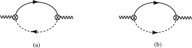
FIGURE 2: Diagrams for the bare susceptibilities in the Peierls (a) and Cooper (b) channels. A continuous (dashed) line correspond to a particle or hole near $+k_{F}$ ($-k_{F}$).

In the static limit, both channels show logarithmic singularities of the form $\chi_{\mu}(T)\sim\ln(E_{F}/T)$ indicating that pair correlations have no characteristic energy scale between $E_{F}$ and $T$. All intermediate scales between $E_{F}$ and $T$ turn out to give similar contributions to the integrals (1.47) and (1.50), which are roughly of the form $\int_{T}^{E_{F}}d\epsilon_{+}/\epsilon_{+}$ at $q=0$ and $\omega_{m}=0$ as shown in Fig. 3, a feature that can be equated with scaling.[1]

FIGURE 3: Energy scales for the 1D fermion problem. Between the Fermi ($E_{F}$) and thermal energy ($T$), there is no characteristic energy scale.

This logarithmic divergence can also be seen as a power law with a vanishing exponent, that is

$$\chi_{\mu}(T)=\lim_{\gamma\rightarrow 0^{+}}-N(0)\gamma^{-1}\Big{[}\Big{(}{T\over 1.13E_{F}}\Big{)}^{-\gamma}-1\Big{]}.$$ (1.52)

According to the relation (1.19), this should imply $\eta\to 2$, namely a logarithmic singularity in $q$. This is indeed consistent with the asymptotic behavior of $\chi_{\mu}(q)$ at $T=0$ and $\omega_{m}=0$, which is found to be

$$\chi_{\mu}(q)=N(0)\ln{|v_{F}q|\over 2E_{F}},$$ (1.53)

in agreement with (1.16).

The origin of scale invariance can be further sharpened if one looks at the decay of the fermion coherence at large distance. Consider the Green’s function

$$G_{p}^{0}(x,\tau) = {T\over L}\sum_{k,\omega_{n}}G_{p}^{0}(k,\omega)\ e^{ikx-i\omega_{n}\tau}$$ (1.54)

$$= {e^{ipk_{F}x}\over 2\pi i}{1\over\xi\ {\sinh[(x+ipv_{F}\tau)/\xi]}}$$ (1.55)

where

$$\xi={v_{F}\over\pi T}$$ (1.56)

is a characteristic length scale for the quantum coherence of each fermion and in fact the de Broglie quantum length. At low temperature for $a\ll x\ll\xi$, one finds the power law decay of coherence as a function of distance

$$G^{0}_{p}(x)\sim 1/x,$$ (1.57)

which signals homogeneity or scaling. Reverting to (1.6), we verify that $\theta=0$ in the free fermion limit. For $x\gg\xi$,

$$G^{0}_{p}(x)\sim e^{-x/\xi}$$ (1.58)

there is no homogeneity and the coherence is exponentially damped with distance. The absence of energy scale between $E_{F}$ and $T$ thus corresponds in real space to the absence of length scale between $\xi$ and $a$. Rewriting the elementary the Cooper and Peierls susceptibilities as

$$\chi_{\mu}(T)\approx-N(0)\ln{\xi\over a},$$ (1.59)

one then sees that the quantum spatial coherence of particles becomes an essential ingredient in building up logarithmic singularities in pair correlations of the Cooper and Peierls channels. This can be directly verified by the decay of pair correlations in space and time. From the definition (1.14) and the use of Wick theorem for free fermions, one obtains

$$\chi_{\mu}(x,\tau) = \mp 2\,G^{0}_{-}(\mp x,\mp\tau)G^{0}_{+}(-x,-\tau)$$ (1.60)

$$= e^{-iq_{0}x}{1\over 2\pi^{2}\xi^{2}}{1\over{\sinh[(x+iv_{F}\tau)/\xi]}\ {\sinh}[(x-iv_{F}\tau)/\xi]},$$ (1.61)

where the upper (lower) sign corresponds to the Cooper (Peierls) case. For $a\ll x\ll\xi$, one finds

$$\chi_{\mu}(x)\propto{e^{iq_{0}x}\over x^{2}},$$ (1.62)

in agreement with (1.15), in which $\bar{d}=2$ and $\eta=2$. At large distance, when $x\gg\xi$, one has

$$\chi_{\mu}(x)\propto e^{iq_{0}x}e^{-2x/\xi},$$ (1.63)

where the effective coherence length for pairs is half the one of a single fermion.

3.2 Interchain coupling

A very simple illustration of a dimensionality crossover for the single-particle coherence can be readily given in the free fermion case by adding an interchain hopping term to the the free action, which becomes

$$S_{0}[\psi^{*},\psi] = S_{0}[\psi^{*},\psi]_{1D}\ +\sum_{\widetilde{k},p,\alpha}\sum_{\langle i,j\rangle}t_{\perp}\psi_{p,\alpha,i}^{*}(\widetilde{k})\psi_{p,\alpha,j}(\widetilde{k})$$ (1.64)

$$= \sum_{{\bf k},\omega_{n}}\sum_{p,\alpha}[G^{0}_{p}({\bf k},\omega_{n})]^{-1}\psi_{p,\alpha}^{*}({\bf k},\omega_{n})\psi_{p,\alpha}({\bf k},\omega_{n})$$ (1.65)

where $t_{\perp}$ is the single-particle hopping integral between nearest-neighbor chains $i$ and $j$. Considering a linear array of $N_{\perp}$ chains, the free propagator that parameterizes $S_{0}$ in Fourier is

$$G^{0}_{p}({\bf k},\omega_{n})=\big{(}i\omega_{n}-E_{p}({\bf k})\big{)}^{-1},$$ (1.66)

where

$$E_{p}({\bf k})=\epsilon_{p}(k)-2t_{\perp}\cos k_{\perp}$$ (1.67)

is the full fermion spectrum. The propagator can be trivially written in the extended scaling scaling form (1.20) with $\bar{\gamma}=1$, where the scaling function takes the simple form

$$X_{G}(y)=(1+y)^{-1},$$ (1.68)

with $y=Bt_{\perp}\cos(k_{\perp})/T$ and $B=(i\pi/2)^{-1}$. This implies $\phi_{x^{1}}=1$ for the single-particle crossover exponent. This value of $\phi_{x^{1}}$ is found in the anisotropic free field theory of critical phenomena.[4] The Fourier transform leads to single-particle fermion correlation function

$$G^{0}_{p}(x,n_{\perp},\tau)=G^{0}_{p}(x,\tau)e^{-i\pi n_{\perp}}J_{n_{\perp}}(x/\xi_{x}),$$ (1.69)

where $n_{\perp}$ is the transverse separation expressed in number of chains. The crossover scaling function is then embodied in the Bessel function $J_{n_{\perp}}(x/\xi_{x})$ of order $n_{\perp}$, which takes sizable values when the intrachain distance $x$ reaches values of the order of the characteristic length scale $\xi_{x}=v_{F}/(2t_{\perp})$ needed for coherent hopping from one chain to another (Figure 1). For $x\sim\xi$, the crossover condition is $\xi\sim\xi_{x}$, and this leads once again to $T_{x^{1}}\sim t_{\perp}$, namely $\phi_{x^{1}}=1$.

4 The Kadanoff-Wilson renormalization group

4.1 One-dimensional case

When the motion of fermions is entirely confined to one spatial dimension, particles cannot avoid each other and hence the influence of interactions is particularly important. The absence of length scale up to $\xi$ found in the free fermion gas problem for both single and pair correlations will carry over in the presence of interactions, which couple different energy scales. The low energy behavior of the system in which we are interested will be influenced by all the higher energy states up to the highest energy at the band edge. Renormalization group ideas can be used to tackle the problem of the cascade of energy or length scales that characterizes interacting fermions. This will be done in the framework of the fermion gas model in which the direct interaction between fermions is parametrized by a small set of distinct scattering processes close to the Fermi level (Figure 4). [9] This is justified given the particular importance shown by the Cooper and Peierls infrared singularities for electronic states near the Fermi level. We will consider the backward ($g_{1}$) and forward ($g_{2}$) scattering processes for which particles on opposite sides of the Fermi level exchange momentum near $2k_{F}$ and zero respectively. When the band is half-filled, $4k_{F}$ coincides with a reciprocal lattice vector, making possible Umklapp processes, denoted by $g_{3}$, in which two particles can be transferred from one side of the Fermi level to the other. Thus, adding the interaction part $S_{I}$ to the action, the partition function in the absence of source fields takes the form

$$Z = \int\!\!\!\int{\cal D}\psi^{*}{\cal D}\psi\ e^{S_{0}[\psi^{*},\psi]+S_{I}[\psi^{*},\psi]}$$ (1.70)

$$= \int\!\!\!\int{\cal D}\psi^{*}{\cal D}\psi\ \exp\Big{\{}\sum_{\widetilde{k},\alpha}[G_{p}^{0}(\widetilde{k})]^{-1}\psi_{p,\alpha}^{*}(\widetilde{k})\psi_{p,\alpha}(\widetilde{k})$$ (1.71)

$$+ \ \pi v_{F}T/L\sum_{\{p,\widetilde{k},\widetilde{q},\alpha\}}g_{\{\alpha\}}\ \psi^{\ast}_{+,\alpha_{1}}(\widetilde{k}_{1}+\widetilde{q})\psi^{\ast}_{-,\alpha_{2}}(\widetilde{k}_{2}-\widetilde{q})\psi_{-,\alpha_{3}}(\widetilde{k}_{2})\psi_{+,\alpha_{4}}(\widetilde{k}_{1})$$ (1.72)

$$- \ \pi v_{F}\ T/2L\sum_{\{p,\widetilde{k},\widetilde{q},\alpha\}}g_{3}\ \psi^{\ast}_{p,\alpha}(\widetilde{k}_{1}+p\widetilde{q})\psi^{\ast}_{-p,\alpha^{\prime}}(\widetilde{k}_{1}-p\widetilde{q}+p\tilde{G})\psi_{-p,\alpha^{\prime}}(\widetilde{k}_{2})\psi_{p,\alpha}(\widetilde{k}_{1})\Big{\}}$$ (1.73)

where

$$g_{\{\alpha\}}=g_{1}\delta_{\alpha_{1}\alpha_{3}}\delta_{\alpha_{2}\alpha_{4}}-g_{2}\delta_{\alpha_{1}\alpha_{4}}\delta_{\alpha_{2}\alpha_{3}}$$ (1.74)

and $\tilde{G}=(4k_{F},0)$ is the reciprocal lattice vector. The parameter space of the action is then

$$\mu_{S}=(G^{0}_{p},g_{1},g_{2},g_{3}).$$ (1.75)

where all the couplings are expressed in units of $\pi v_{F}$.

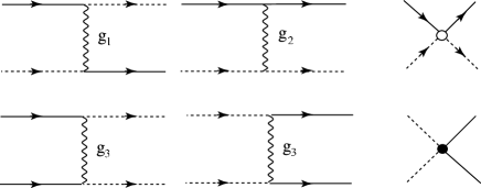
FIGURE 4: Backward ($g_{1}$), forward ($g_{2}$) and umklapp ($g_{3}$) couplings of the 1-D fermion gas model and the corresponding diagrams. The open (full) circle corresponds to the generic vertex part for backward and forward (umklapp) scatterings.

The idea behind the Kadanoff-Wilson renormalization group is the transformation or renormalization of the action $S$ following successive partial integration of $\bar{\psi}^{\prime}$s of momentum located in the energy shell $\frac{1}{2}E_{0}(\ell)d\ell$ on both sides of the Fermi level, where $E_{0}(\ell)=E_{0}e^{-\ell}$ is the effective bandwidth at step $\ell$ of integration and $d\ell\ll 1$. The transformation of $S$ from $\ell$ to $\ell+d\ell$, that keeps the partition function invariant is usually written as

$$Z= e^{A(\ell)}\int\!\!\!\int_{<}{\cal D}\psi^{*}{\cal D}\psi e^{S[\psi^{*},\psi]_{<}}\ \int\!\!\!\int{\cal D}\bar{\psi}^{*}{\cal D}\bar{\psi}\,e^{S[\psi^{*},\psi,\bar{\psi}^{*},\bar{\psi}]_{d\ell}}$$ (1.76)

$$= e^{A(\ell+d\ell)}\int\!\!\!\int_{<}{\cal D}\psi^{*}{\cal D}\psi e^{S[\psi^{*},\psi]_{\ell+d\ell}},$$ (1.77)

where $A(\ell)$ corresponds to the free energy density at the step $\ell$. The integration measure in the outer shell is

$${\cal D}\bar{\psi}^{*}{\cal D}\bar{\psi}=\prod_{p,\alpha,\{\widetilde{k}\}^{\prime}}d\bar{\psi}^{*}_{p,\alpha}(\widetilde{k})d\bar{\psi}_{p,\alpha}(\widetilde{k}).$$ (1.78)

and $\{\widetilde{k}\}^{\prime}=\{k\}^{\prime}\{\omega_{n}\}$. Here $\{k\}^{\prime}$ corresponds to the momentum outer shells

$$\ k_{0}e^{-\ell}+k_{F}>k>k_{0}e^{-\ell-d\ell}+k_{F}\ \ \ \ \ \ \ \ \ \ (-k_{0}e^{-\ell-d\ell}-k_{F}>k>-k_{0}e^{-\ell}-k_{F})$$

above the Fermi level and

$$-k_{0}e^{-\ell-d\ell}+k_{F}>k>-k_{0}e^{-\ell}+k_{F}\ \ \ \ \ (-k_{0}e^{-\ell}-k_{F}>k>-k_{0}e^{-\ell-d\ell}-k_{F})$$

below for right (left) moving fermions, while $\{\omega_{n}\}$ covers all the Matsubara frequencies. The remaining inner shell ($<$) fermion degrees of freedom are kept fixed. The parameters of the action denoted as $\mu_{S}$ transform according to

$$R_{d\ell}\,\mu_{S}(\ell)=\mu_{S}(\ell+d\ell).$$ (1.79)

where

$$\mu_{S}(\ell)=\big{(}z(\ell)G_{p}^{0},z_{1}(\ell)g_{1},z_{2}(\ell)g_{2},z_{3}(\ell)g_{3})$$ (1.80)

contains the factors $z$ and $z_{i=1,2,3}$ that renormalize the parameter space of the action at $\ell$.[44] The flow of parameters is conducted down to $\ell_{T}\equiv\ln E_{F}/T$ corresponding to the highest value of $\ell$ at which scaling applies as discussed in § II. This leads in turn to the temperature dependence of the parameter space $\mu_{S}(T)$. It should be mentioned that the Kadanoff transformation will generate new terms which were not present in the action at $\ell=0$. In principle, the relevance of these can be seen explicitly from a rescaling of energy and field ‘density’ after each partial integration. Thus performing an energy change by the factor $s=e^{d\ell}>1$, one has

$$\epsilon_{p}^{\prime}= s\epsilon_{p}$$ (1.81)

$$\omega_{n}^{\prime}= s\omega_{n}.$$ (1.82)

The fermion fields in the action will then transform according to

$$\psi^{\prime(*)}=z^{-\frac{1}{2}}s^{-\frac{1}{2}}\psi^{(*)},$$ (1.83)

which in its turn implies that the rescaling of interaction parameters is given by

$$g_{i}^{\prime}=g_{i}\,z_{i}\,z^{2},\ \ \ \ \ {\rm for}\ \ \ \ {i=1,2,3}.$$ (1.84)

This contains only anomalous renormalization factors indicating that the interaction parameters are all marginal. However, if interactions between three, four or more particles were added to the bare action, the amplitude of these would decay as $1/s$ to some positive power, and would therefore be irrelevant in the RG sense. A different conclusion would be reached, however, if these many-body interactions were generated in the flow of renormalization. In this case, the amplitudes of interactions becomes scale dependent and such couplings can remain marginal or even become relevant (see § 4.3 and § 5.1). Besides this use, rescaling for our fermion problem is not an essential step of the RG transformation. We will consider the renormalization of $\mu_{S}$ with respect to $\ell$ as a transformation that describes an effective system with a reduced band width $E_{0}(\ell)$ or a magnified length scale $v_{F}/E_{0}(\ell)$.

In practice, the partial integration (1.77) is most easily performed with the aid of diagrams. We first decompose the ${\widetilde{k}}$ sums in the action into outer and inner shells momentum variables

$$\sum_{\{\widetilde{k}\}}=\sum_{\{\widetilde{k}\}^{\prime}}+\sum_{\{\widetilde{k}\}_{<}}.$$ (1.85)

This allows us to write

$$S[\psi^{*},\psi]=S[\psi^{*},\psi]_{<}+S[\psi^{*},\psi,\bar{\psi}^{*},\bar{\psi}]$$ (1.86)

where $S[\psi^{*},\psi]_{<}$ of the action with all the $\psi^{\prime}$s in the inner shell, whereas

$$S[\psi^{*},\psi,\bar{\psi}^{*},\bar{\psi}]=S_{0}[\bar{\psi}^{*},\bar{\psi}]+\sum_{i=1}^{4}S_{I,i}[\psi^{*},\psi,\bar{\psi}^{*},\bar{\psi}]$$ (1.87)

consists in a free part in the outer momentum shell and an interacting part as a sum of terms, $S_{I,i}$, having $i=1,\ldots 4$ $\bar{\psi}^{\prime}$s in the outer momentum shell. Their integration following the partial trace operation (1.77) is performed perturbatively with respect to $S_{0}[\bar{\psi}^{*},\bar{\psi}]$. Making use of the linked cluster theorem, the outer shell integration becomes

$$Z=e^{A(\ell)}\int\!\!\!\int_{<}{\cal D}\psi^{*}{\cal D}\psi e^{S[\psi^{*},\psi]_{<}}\int\!\!\!\int{\cal D}\bar{\psi}^{*}{\cal D}\bar{\psi}\,e^{S_{0}[\bar{\psi}^{*},\bar{\psi}]}\,\exp\Big{\{}\sum_{i=1}^{4}S_{I,i}[\psi^{*},\psi,\bar{\psi}^{*},\bar{\psi}]\Big{\}}$$ (1.88)

$$\ \ \ =e^{A(\ell)}\int\!\!\!\int_{<}{\cal D}\psi^{*}{\cal D}\psi\exp\Big{\{}S[\psi^{*},\psi]_{<}+\sum_{n=1}^{\infty}1/n!\,\langle(\,\sum_{i}S_{I,i}[\psi^{*},\psi,\bar{\psi}^{*},\bar{\psi}]\,)^{n}\rangle_{\bar{0},c}\Big{\}}$$ (1.89)

where

$$\langle....\rangle_{\bar{0},c}=Z^{-1}_{\bar{0}}\int\!\!\!\int{\cal D}\bar{\psi}^{*}{\cal D}\bar{\psi}\,(.....)\,e^{S_{0}[\bar{\psi}^{*},\bar{\psi}]}$$ (1.90)

is a free fermion average corresponding to a connected diagram evaluated in the outer momentum shell and

$$Z_{\bar{0}}=\int\!\!\!\int{\cal D}\bar{\psi}^{*}{\cal D}\bar{\psi}\,e^{S_{0}[\bar{\psi}^{*},\bar{\psi}]},$$ (1.91)

is the outer shell contribution to the free partition function.

4.2 One-loop results

The KW method may be used to obtain low order results presented in previous review papers,[15, 16] and no particular technical difficulties arise. The following two subsections present material which has already been developed using the parquet summation[8, 9] and the first order multiplicative renormalization group.[10, 45, 11] Nevertheless, it is useful to supply the basic properties of the logarithmic theory of the 1D fermion gas model using this method.

Incommensurate band filling

For band filling that is incommensurate, there is no possibility of Umklapp scattering so that one can drop $g_{3}$ in the action. The renormalization of backward and forward scattering amplitudes at the one-loop level are obtained from the $n=2$ outer-shell averages $\frac{1}{2}\langle(S_{I,2})^{2}\rangle$, where

$$S_{I,2}[\psi^{\ast},\psi,\bar{\psi}^{\ast},\bar{\psi}]\ = S_{I,2}^{C}+S_{I,2}^{P}+S_{I,2}^{L}$$ (1.92)

$$\Longleftrightarrow \ (\bar{\psi}_{+}^{\ast}\bar{\psi}_{-}^{\ast}\psi_{-}\psi_{+}+{\rm c.c})+\,(\bar{\psi}_{+}^{\ast}\psi^{*}_{-}\bar{\psi}_{-}\psi_{+}+{\rm c.c})$$ (1.93)

$$\ + s\ (\bar{\psi}_{+}^{\ast}{\psi}_{-}^{\ast}\psi_{-}\bar{\psi}_{+}+{\psi}_{+}^{\ast}\bar{\psi}_{-}^{\ast}\bar{\psi}_{-}{\psi}_{+}),$$ (1.94)

the three terms of which correspond to putting two particles or two holes in the outer momentum shell (the Cooper channel), one particle and one hole on opposite branches (the Peierls channel), and finally putting a particle and a hole on the same branch (the Landau channel). The latter does not lead to logarithmic contributions at the one-loop level and can be ignored for the moment. The flow of the scattering amplitudes becomes $g_{i=1,2}(\ell+d\ell)=z_{i=1,2}(d\ell)g_{i=1,2}(\ell)$ where the renormalization factors at the one-loop level are

$$z_{1}(d\ell) = 1-2g_{1}(\ell)\,I_{P}(d\ell)+2g_{2}(\ell)\,[I_{P}(d\ell)+I_{C}(d\ell)]$$ (1.95)

$$z_{2}(d\ell) = 1+g_{2}^{-1}(\ell)g_{1}^{2}(\ell)\,I_{C}(d\ell)+g_{2}(\ell)\,[I_{P}(d\ell)+I_{C}(d\ell)].$$ (1.96)

The outer shell integration of the Peierls channel at $2k_{F}$ and zero external frequency enables the particle and hole to be simultaneously in the outer-shell. The result is

$$I_{P}(d\ell) = -\pi v_{F}{T\over L}\sum_{\{\widetilde{k}\}^{\prime}}G^{0}_{+}(k,\omega_{n})G_{-}^{0}(k-2k_{F},\omega_{n})$$ (1.97)

$$= \left\{\int_{-\frac{1}{2}E_{0}(\ell)}^{-\frac{1}{2}E_{0}(\ell+d\ell)}\!\!\!+\int_{\frac{1}{2}E_{0}(\ell+d\ell)}^{\frac{1}{2}E_{0}(\ell)}\right\}{\tanh(\frac{1}{4}\beta E_{0}(\ell))\over E_{0}(\ell)}\,dE_{0}(\ell)$$ (1.98)

$$\simeq \frac{1}{2}d\ell.$$ (1.99)

Similarly in the Cooper channel at zero pair momentum and external frequency, we have

$$I_{C}(d\ell) = \pi v_{F}{T\over L}\sum_{\{\widetilde{k}\}^{\prime}}G^{0}_{+}(k,\omega_{n})G_{-}^{0}(-k,-\omega_{n})$$ (1.100)

$$= -I_{P}(d\ell).$$ (1.101)

Both contributions are logarithmic and their opposite signs lead to important cancellations (interference). The diagrams which remain after the cancellation are shown in Fig. 5.

FIGURE 5: Recursion relations for backward ($g_{1}$) and forward ($g_{2}$) scattering at the one-loop level. The slashed lines refer to a particle or a hole in the outer shell.

With an obvious rearrangement, the flow equations may be written

$${dg_{1}\over d\ell}=-g_{1}^{2}$$ (1.102)

$${d\over d\ell}(2g_{2}-g_{1})=0.$$ (1.103)

The solution for $g_{1}(\ell)$ is found at once to be

$$g_{1}(\ell)={g_{1}\over 1+g_{1}\ell},$$ (1.104)

showing that backward scattering is marginally irrelevant (relevant) if the bare coupling $g_{1}$ is repulsive (attractive). As for the combination $2g_{2}-g_{1}$, it remains marginal, an invariance that reflects the conservation of particles on each branch.[46, 47] Another feature of these equations is the fact that the flow of $g_{1}$ is entirely uncoupled from the one of $2g_{2}-g_{1}$. This feature, which follows from the interference between the Cooper and the Peierls channels, gives rise to an important property of 1D interacting fermion systems, namely the separation of long wavelength spin and charge degrees of freedom. This is rendered manifest by rewriting the interacting part of the action as follows[9]

$$S_{I}[\psi^{*},\psi]_{\ell}\ =-\pi v_{F}(2g_{2}-g_{1})\sum_{p,\widetilde{q}}\rho_{p}(\widetilde{q})\rho_{-p}(-\widetilde{q})+\,\pi v_{F}\,g_{1}(\ell)\sum_{p,\widetilde{q}}{\bf S}_{p}(\widetilde{q})\cdot{\bf S}_{-p}(-\widetilde{q})$$ (1.105)

where the long-wave length particle-density and spin-density fields of branch $p$ are defined by

$$\rho_{p}(\widetilde{q}) = \frac{1}{2}\sqrt{T\over L}\sum_{\alpha,\{\widetilde{k}\}_{<}}\psi^{*}_{p,\alpha}(\widetilde{k}+\widetilde{q})\psi_{p,\alpha}(\widetilde{k})$$ (1.106)

$$\ \ \ \ {\bf S}_{p}(\widetilde{q}) = \frac{1}{2}\sqrt{T\over L}\sum_{\alpha,\{\widetilde{k}\}_{<}}\psi^{*}_{p,\alpha}(\widetilde{k}+\widetilde{q})\,\vec{\sigma}^{\alpha\beta}\,\psi_{p,\beta}(\widetilde{k}).$$ (1.107)

The spin-charge separation is preserved at higher order and is a key property of a Luttinger liquid in one dimension.[48] In the repulsive sector $g_{1}\geq 0$, the spin coupling goes to zero, while the forward scattering $g_{2}^{*}(\ell\to\infty)\to g_{2}-g_{1}/2$ flows to a non universal value on the Tomanaga-Luttinger line of fixed points $g_{1}^{*}=0$ (Figure 6).

For an attractive interaction $g_{1}<0$, an instability occurs in the the spin sector at $\ell_{\sigma}$ defined by $g_{1}\ell_{\sigma}=-1$. Identifying $\ell$ with $\ell_{T}=\ln E_{F}/T$, the temperature dependence of the Peierls or Cooper loop, the characteristic temperature scale for strong coupling is

$$T_{\sigma}=E_{F}e^{-1/\mid g_{1}\mid}\equiv\frac{1}{2}\Delta_{\sigma},$$ (1.108)

where $\Delta_{\sigma}$ is defined as the spin gap. According to (1.105), backward scattering can be equated with an exchange interaction between right- and left-going spin densities which is antiferromagnetic in character when $g_{1}$ is attractive. Therefore strong attractive coupling signals the presence of a spin gap $\Delta_{\sigma}$. Although the divergence in (1.104) is an artefact of the one-loop approximation, the flow of $g_{1}(\ell)$ to strong coupling is nevertheless preserved at higher order. This is shown by the fact that the system inevitably crosses the so-called Luther-Emery line at $g_{1}(\ell_{LE})=-6/5$ (Figure 6), where an exact solution using the technique of bosonization confirms the existence of a spin gap.[49, 50]

FIGURE 6: Flow of coupling constants in the $g_{1}g_{2}$ plane at the one-loop level. In the repulsive region $g_{1}\geq 0$, the system has a line of fixed points on the Tomonaga-Luttinger line $g_{1}^{*}=0$. In the attractive sector $g_{1}<0$, the flows is to strong coupling. The dashed line corresponds to the Luther-Emery line at $g_{1}=-6/5$.

Umklapp scattering at half-filling

At half-filling, there is one fermion per site so that $4k_{F}=2\pi/a$ coincides with a reciprocal lattice vector $G$ enabling Umklapp scattering processes denoted by $g_{3}$ in Figure 4. The presence of $g_{3}$ processes reinforces the importance of the $2k_{F}$ density-wave channel compared to the superconducting one. Flows will be modified accordingly. Thus at the one-loop level, the outer shell corrections coming from $\frac{1}{2}\langle(S_{I,2})^{2}\rangle_{\bar{0},c}$ will include additional contributions

$$S_{I,2}\Longleftrightarrow S_{I,2}\big{|}_{g_{3}=0} + (\,\bar{\psi}_{+}^{\ast}{\psi}_{+}^{\ast}\bar{\psi}_{-}\psi_{-}+{\rm perm.}+{\rm c.c}\,)$$ (1.109)

$$+ (\,\bar{\psi}_{+}^{\ast}\bar{\psi}_{+}^{\ast}{\psi}_{-}\psi_{-}+\,{\psi}_{+}^{\ast}{\psi}_{+}^{\ast}\bar{\psi}_{-}\bar{\psi}_{-}+{\rm c.c}\,)$$ (1.110)

involving outer shell fields in the Peierls channel and pairs of particles or holes on the same branch. At the one-loop level only the former gives rise to logarithmic corrections, whereas the latter will be involved in higher order corrections (§ 4.3). The former contributions, along with (1.96), will lead to the recursion formulas $g_{i=1,2,3}(\ell+d\ell)=z_{i=1,2,3}(d\ell)g_{i=1,2,3}(\ell)$, which can be written in form

$$g_{1}(\ell+d\ell) = g_{1}(\ell)-\,2g^{2}_{1}(\ell)I_{P}(d\ell),$$ (1.111)

$$\bigl{(}2g_{2}-g_{1}\bigr{)}(\ell+d\ell) = (2g_{2}-g_{1}\bigr{)}(\ell)+\,2g^{2}_{3}(\ell)I_{P}(d\ell),$$ (1.112)

$$g_{3}(\ell+d\ell) = g_{3}(\ell)+2\bigl{(}2g_{2}-g_{1}\bigr{)}(\ell)g_{3}(\ell)I_{P}(d\ell).$$ (1.113)

The flow of the coupling constants are then governed by

$${dg_{1}\over d\ell} = -g^{2}_{1},$$ (1.114)

$${d\over d\ell}(2g_{2}-g_{1}) = g^{2}_{3},$$ (1.115)

$${dg_{3}\over d\ell} = g_{3}(2g_{2}-g_{1}),$$ (1.116)

which corresponds to the diagrammatic parquet summation of Dzyaloshinskii and Larkin. [9] By combining the last two equations, the flow is found to follow the hyperbolas described by the renormalization invariant $C=[(2g_{2}-g_{1})(\ell)]^{2}-g_{3}^{2}(\ell)$. Umklapp scattering is then entirely uncoupled from $g_{1}$ and will only affect the charge sector. When $g_{1}-2g_{2}>\mid g_{3}\mid$, $g_{3}(\ell)$ scales to zero and is marginally irrelevant, while $2g_{2}^{*}-g_{1}^{*}$ is non universal. The excitation of charge degrees of freedom are then gapless in this case. The attractive Hubbard model in which $g_{1,2,3}=U<0$ falls in this category.

Otherwise, the flows of $g_{3}$ and $2g_{2}-g_{1}$ evolve to strong coupling and both couplings are marginally relevant. There is a singularity at $\ell_{\rho}$ corresponding to the temperature scale

$$T_{\rho}=E_{F}\,e^{-1/\sqrt{\mid C\mid}}\,\equiv\frac{1}{2}{\Delta_{\rho}}.$$ (1.117)

Following the example of the incommensurate case, the couplings inevitably cross the Luther-Emery line at $g_{1}-2g_{2}=-6/5$, at which point the problem can be solved exactly and the existence of a charge gap $\Delta_{\rho}$ is confirmed.[49] The special case of the repulsive Hubbard limit at half-filling where $g_{1,2,3}=U>0$ falls on the separatrix $2g_{2}-g_{1}=\mid g_{3}\mid$ (Figure 7). In this case the solution of (1.116) leads to a singularity at $T_{\rho}=E_{F}e^{-1/\mid g_{3}\mid}$. A charge gap $\Delta_{\rho}$ is consistent with the characteristics of a 1D Mott insulator found in the Lieb-Wu exact solution. [51, 9, 52]

FIGURE 7: The flow of couplings in the charge sector. The condition $g_{1}-2g_{2}>\mid g_{3}\mid$ corresponds to weak coupling where Umklapp scattering is a marginally irrelevant coupling. Otherwise, both $g_{1}-2g_{2}$ and $g_{3}$ are marginally relevant. The Luther-Emery line is located at $g_{1}-2g_{2}=-6/5$.

4.3 Two-loop results

At the one-loop level, corrections to the action parameters $\mu_{S}$ resulting from the partial trace are confined to the scattering amplitudes $g_{i=1,2,3}(\ell)$ and aside from a renormalization of the chemical potential, the flow leaves the single particle properties unchanged. At the two-loop level, outer shell logarithmic contributions will affect both the one-particle self-energy and the four-point vertices. This yields an essential feature of the 1D electron gas model which is the absence of quasi-particle states.

One-particle self-energy

Let us consider first the one-particle part. It is easy to see that the term $\frac{1}{2}\langle(S_{I,3})^{2}\rangle_{\bar{0},c}$ at $n=2$ has the form of a one-particle self-energy correction. However, if we strictly follow the classical Wilson scheme, the constraint of having all internal lines in the outer shell leads to a vanishing contribution. It becomes clear then that one-particle corrections can only be logarithmic at the two-loop level if the internal lines refer to different momentum shells. In the classical Wilson scheme, this possibility actually results from a cascade of contractions on the three-particle interaction (Figure 8). Such interactions, although absent in the initial action, are generated along the RG flow and enlarge the parameter space.

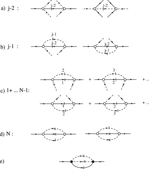
FIGURE 8: The cascade of contractions contributing to logarithmic one-particle self-energy corrections in the local approximation for the RG flow: (a) backward and forward scattering contributions to the three-particle interactions; $\lambda^{+}$ (left) and $\lambda^{-}$ (right) from $\frac{1}{2}\langle S^{2}_{I,1}\rangle_{\bar{0},c}$ at the step $(j-2)$ where $j\geq 3$; (b) second contraction in the outer shell at the step $j-1$ with two internal lines on successive energy shells (only shown for $\lambda^{+}$) ; (c) the summation of diagrams given in (b) up to $j=N-1$ ; (d) outer shell one-particle self-energy correction at the step $N\ (Nd\ell=e^{\ell+d\ell})$ for the top inner shell state $k$ of the $+k_{F}$ branch in the local approximation. Here a crossed (slashed) line refers to fermions in the interval $[0,\ell]$ ($[\ell,\ell+d\ell]$); (e) the result of a similar cascade of contractions for Umklapp scattering.

In order to see how these interactions are generated from the partial trace (1.89) and under what conditions they give rise to logarithmic corrections at the two-loop level, it is useful to label the steps of the outer shell integration by the index $j$, for which $E_{0}(\ell_{j})=E_{0}e^{-(j-2)d\ell}$ is the scaled bandwidth at $j\geq 3$. Thus at each step $j-2$, the contraction $\frac{1}{2}\langle S^{2}_{I,1}\rangle_{\bar{0},c}$ yields a three-particle term in the action (Figure 8-a), which is denoted $\delta S^{(j)}_{\lambda}$. Its explicit expression for the forward and backward scattering is given in Eq. (227) of § 1.1. The analogous expression $\delta S_{\lambda u}^{(j)}$ for Umklapp with $\lambda^{\pm}_{u}$ as the scattering amplitudes is given in (246) of § 1.2. Owing to the presence of the internal line, the rescaling of energy and fields shows that the amplitudes $\lambda^{\pm}$ and $\lambda_{u}^{\pm}$ are marginal.[24] At the next step of partial integration $j-1$, two fermion fields of these three-particle terms can in turn be contracted in $\langle\delta S^{(j)}_{\lambda,2}\rangle_{\bar{0},c}$, from which we will retain an effective two-particle interaction with two internal lines tied to the adjacent shells $j-2$ and $j-1$ (Figure 8-b and (234)). These contributions are non-logarithmic and differ from those already retained in the one-loop calculation in §4.2 for which both internal lines were put in the same outer shell. The repetition of these contractions is carried out by a sum on $j$ up to $N-1$ (Figure 8-c), which yields $\delta S^{\prime}_{\lambda}\equiv\sum_{j}^{N-1}\langle\delta S^{(j)}_{\lambda,2}\rangle_{\bar{0},c}$ ($\delta S^{\prime}_{\lambda,u}\equiv\sum_{j}^{N-1}\langle\delta S^{(j)}_{\lambda,u,2}\rangle_{\bar{0},c}$ for Umklapp) as shown in (234) ((247) for Umklapp). At the next step, $N$, of partial integration, two more fields are in turn contracted which lead to a sum of one-particle self-energy corrections for a $k$ state at the top of the inner shell.[53] Since each term of the sum refers to couplings at different steps $j$, the correction is non-local.

In the following, we will adopt a local scheme of approximation, which consists in neglecting the slow (logarithmic) variation of the coupling constants in the intermediate integral over momentum transfer $q$ in (242) and evaluate them at $\ell$ (Figure 8-d). It is worth noting that the local approximation becomes exact for couplings or combination of couplings that are invariant with respect to $\ell$. This turns out to be the case for the Tomanaga-Luttinger model when only $g_{2}$ coupling is present ($g_{1}=g_{3}=0$), or for the combination $2g_{2}-g_{1}$ when $g_{3}=0$. Neglecting small scaling deviations, the end result given by (242) ((248) for Umklapp) is logarithmic and contributes to a $1/z$ renormalization factor of $[G_{p}^{0}(k,\omega_{n})]^{-1}$ for $k$ located at the top of the inner shell. The flow equation for $z(\ell)$ is

$${d\over d\ell}\ln z=-{1\over 16}[(2g_{2}-g_{1})^{2}+3g_{1}^{2}+2g_{3}^{2}].$$ (1.118)

The solution as a function of $\ell$ can be written as a product $z=z_{\sigma}z_{\rho}$ of renormalization factors, in which

$$z_{\sigma}(\ell)=\exp\Big{\{}-{3\over 16}\int_{0}^{\ell}g_{1}^{2}d\ell^{\prime}\Big{\}}$$ (1.119)

for the spin part and

$$z_{\rho}(\ell)=\exp\Big{\{}-{1\over 16}\int_{0}^{\ell}[(2g_{2}-g_{1})^{2}+2g_{3}^{2}]d\ell^{\prime}\Big{\}}$$ (1.120)

for the charge. Prior to analyzing the impact of these equations on one-particle properties, to work consistently at two-loop order, we must proceed to the evaluation of the two-loop contribution to the coupling constant flow.

Four-point vertices

To obtain the two-loop corrections to four-point vertices within a classical KW scheme, we come up against difficulties similar to those found for the one-particle self-energy. We can indeed verify that contractions of the form $\langle S_{I,3}^{2}S^{L}_{I,2}\rangle_{\bar{0},c}$ at $n=3$, which would lead to two-loop corrections for the four-point vertices, are actually vanishingly small if all internal lines are in the same momentum shell. Here again non-zero contributions can only be found if the internal lines refer to different shells, which implies that the contractions must be made starting from interactions that involve more than two particles (Figure 9).[15] Here we skip the technical details of the calculation and only sketch the main steps, which run parallel to those of the one-particle self-energy. The cascade of contractions starts from the four-particle interaction resulting from ${3\over 3!}\langle S_{I,2}^{L}S_{I,1}S_{I,1}\rangle_{\bar{0},c}$ at $n=3$, which involves the contribution $S_{I,2}^{L}$ of the Landau channel. The corresponding diagrams are shown in Figure 9-a at the step $j-2$. For the required contractions to be possible, the momentum transfer must be zero. At the next step, two more fields are contracted and a line is put in the adjacent shell $j-1$ (Figure 9-b). As a function of $j$, these corrections add up as shown in Figure 9-c to lead to effective three-particle interactions at the step $N-1$. At the last step, $N$, of the cascade, one arrives at a two-loop correction for the four-point vertices (Figure 9-d). Following the example of one-particle self-energy, these corrections are non-local in the coupling constants. In the local approximation scheme, one finds an outer shell contribution that is ${\cal O}(g^{3}d\ell)$ (Figure 9-d). The two-loop contributions involving Umklapp scattering are shown in Figure 9-e. Finally, the outer shell contributions to the renormalization factors $z_{1,2,3}$ (neglecting corrections to logarithmic scaling at $\ell$) are given by

$$z^{(2)}_{1}(d\ell) = 1/4\Bigl{(}g^{2}_{3}(\ell)+2g_{2}(\ell)\bigl{(}g_{2}(\ell)-g_{1}(\ell)\bigr{)}\Bigr{)}d\ell,$$ (1.121)

$$z^{(2)}_{2}(d\ell) = -g^{-1}_{2}(\ell)/4\Bigl{(}g^{3}_{1}(\ell)-2g^{2}_{1}(\ell)g_{2}(\ell)+2g^{2}_{2}(\ell)g_{1}(\ell)$$ (1.122)

$$- 2g^{2}_{2}(\ell)+g^{2}_{3}(\ell)\bigl{(}g_{2}(\ell)-g_{1}(\ell)\bigr{)}\Bigr{)}d\ell,$$ (1.123)

$$z^{(2)}_{3}(d\ell) = 1/4\bigl{(}g^{2}_{1}(\ell)+2g_{1}(\ell)g_{2}(\ell)-2g^{2}_{2}(\ell)\bigr{)}.$$ (1.124)

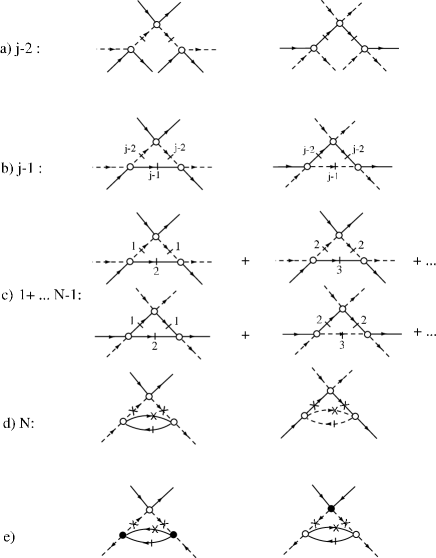
FIGURE 9: The cascade of contractions contributing to the four-point vertices in the local approximation of the RG flow: (a) backward and forward scattering contributions to the generation of four-particle interactions from ${1\over 2}\langle S_{I,2}^{L}S_{I,1}S_{I,1}\rangle_{\bar{0},c}$ at the step $j-2$ ($j\geq 3$) ; (b) second contraction in the outer shell at the step $j-1$ ; (c) the summation of diagrams given in (b) up to $j=N-1$ as effective three-particle interactions; (d) two-loop outer shell correction to four-point vertices in the local approximation at the step $Nd\ell\to\ell+d\ell$. Here a crossed (dashed) line refers to fermion lines in the interval $[0,\ell]$ ($[\ell,\ell+d\ell]$); (e) the result of a similar cascade of contractions for Umklapp scattering.

Now, combining these with the one-loop results of (1.116) and performing the rescaling of the fields, one has $z^{-1/2}\psi^{(*)}\rightarrow\psi^{(*)}$

$$\mu_{S}=(G_{p}^{0},z_{1}z^{2}g_{1},z_{2}z^{2}g_{2},z_{3}z^{2}g_{3},\ldots),$$ (1.125)

which renders explicit the renormalization of the couplings $g_{i}$. Neglecting scaling deviations at small $\ell$, the corresponding scaling equations are

$${dg_{1}\over d\ell} = -g^{2}_{1}-{1\over 2}g^{3}_{1},$$ (1.126)

$${d\over d\ell}(2g_{2}-g_{1}) = g^{2}_{3}[1-{1\over 2}(2g_{2}-g_{1})],$$ (1.127)

$${dg_{3}\over d\ell} = g_{3}(2g_{2}-g_{1})[1-{1\over 4}(2g_{2}-g_{1})]-{1\over 4}g^{3}_{3},$$ (1.128)

which reproduces the old results of the multiplicative renormalization group method. [11, 45] We see that the spin coupling $g_{1}$ is still uncoupled to the charge couplings $2g_{2}-g_{1}$ and $g_{3}$. Furthermore, the one-loop singularities, previously found at $T_{\nu=\sigma,\rho}$, are removed and replaced by strong coupling fixed points for the couplings as $\ell\rightarrow\infty$. For the interesting cases already analyzed at the one loop level, we have first the attractive one where $g_{1}<0$ and $g_{1}-2g_{2}>\,\mid g_{3}\mid$, for which $g_{1}^{*}\to-2$, $g_{3}^{*}\to 0$, while $g^{*}_{1}-2g^{*}_{2}$ is strongly attractive but non universal; second, in the repulsive case when $g_{1}>0$ and $g_{1}-2g_{2}<\,\mid g_{3}\mid$, for which Umklapp is marginally relevant with $g^{\ast}_{3}\to 2,g^{\ast}_{2}\rightarrow 1$ and $g^{\ast}_{1}\rightarrow 0$. Since in both cases, the couplings cross the Luther-Emery line, the scale for the gap $\Delta_{\nu}$ remains of the order of the one-loop temperature scale $T_{\nu}$ in both sectors.

The integration of (1.118) at large $\ell\gg\ell_{\nu}$ then leads to the power law decay

$$z(\ell)\sim\bigl{(}E_{0}(\ell)/\Delta_{\nu}\big{)}^{\theta^{\ast}}.$$ (1.129)

The exponent evaluated at the fixed point in the presence of a single gap can be separated into charge ($\theta_{\rho}$) and spin ($\theta_{\sigma}$) components:

$$\theta^{\ast} =\theta^{\ast}_{\rho}(2g^{*}_{2}-g_{1}^{*},g^{*}_{3})+\theta^{*}_{\sigma}(g^{*}_{1})$$ (1.131)

$$\simeq 3/4.$$

The case when there is no Umklapp and $g_{1}>0$ corresponds to the Tomonaga-Luttinger model at large $\ell$. The couplings remain weak and one finds the power law decay

$$z(\ell)=D_{\sigma}(\ell)\Bigl{(}E_{0}(\ell)/E_{0}\Bigr{)}^{\theta_{\rho}},$$ (1.132)

with

$$\theta_{\rho}={1\over 16}(2g_{2}-g_{1})^{2},$$ (1.133)

and

$$D_{\sigma}(\ell)=\exp\Big{(}-{3\over 16}\int^{\ell}_{0}g_{1}^{2}(\ell^{\prime})d\ell^{\prime}\Big{)}.$$ (1.134)

Here the exponent $\theta_{\rho}$ is non-universal.[11] A contribution from the spin degrees of freedom appears through the weak transient $D_{\sigma}(\ell)$. The physics of this gapless case is that of the Luttinger liquid.

The factor $z$ is the quasi-particle weight at Fermi level. In all cases, it vanishes at $\ell\to\infty$ or $T\to 0$ indicating the absence of a Fermi liquid in one-dimension. Actually the same factor also coincides with the single-particle density of states at the Fermi level

$$N^{*}(\ell)=N(0)z(\ell),$$ (1.135)

which vanishes in the same conditions.

The connection between the one-particle Green’s function computed at $\ell=0$ and that computed at non-zero $\ell$ can be written in the form

$$G_{p}(\widetilde{k},\mu_{S})=z(\ell)G_{p}(\widetilde{k},\mu_{S}(\ell)).$$ (1.136)

When $\ell\to\infty$, the number of degrees of freedom to be integrated out goes to zero, thus $G_{p}(\widetilde{k},\mu_{S}(\ell))\to zG^{0}_{p}(k\to k_{F},\omega_{n})$ and as a function of $T\to 0$, one finds

$$G_{p}(k_{F},\omega_{n=0},\mu_{S})\approx C{T}^{-\bar{\gamma}},$$ (1.137)

where, consistent with the scaling ansatz (1.7), $\bar{\gamma}=1-\theta$ and $C=1/(i\pi E_{F}^{\theta})$. If we identify the vanishing energy $\frac{1}{2}E_{0}(\ell)$ in $z(\ell)$ with $v_{F}(pk-k_{F})$ close to $k_{F}$, we have at $T=0$

$$G_{p}(k,\mu_{S})\propto\ \mid pk-k_{F}\mid^{-1+\theta},$$ (1.138)

which agrees with the scaling expressions (1.5-1.6) showing the absence of a Fermi liquid.

Remarks

At this point, casting a glance back at the RG approach described above, a few remarks can be made in connection with the alternative formulation presented in Refs. [15, 16] In the classical Wilsonian scheme presented here, a momentum cutoff $k_{0}$ (or bandwidth $E_{0}$) is imposed on the spectrum at the start and all contractions done at a given step of the RG refer to fermion states of the outer shell tied to that particular step. In this way, we have seen that the two-loop level calculations require a cascade of outer shell contractions starting from many-particle interactions that were not present in the bare action. The cascade therefore causes non-locality of the flow which depends on the values of coupling constants obtained at previous steps. Thus obtaining logarithmic scaling at higher than one-loop forces us to resort to a local approximation.

In the formulation of Refs. [15, 16], the Kadanoff transformation at high order is performed differently. In effect, a cutoff $k_{0}$ is not imposed on the range of momentum for the spectrum in the free part of the action $S_{0}$ but it only bounds the $k$-summations of the interaction term $S_{I}$. The latter summations, of which there two in both of the interaction terms (as in Eqn. (1.73) ), are involved in the ultraviolet regularization of all singular diagrams, while the remaining summation on the momentum transfer $q$ is treated independently. In this way, the interaction term $S_{I}[\psi^{*},\psi,\bar{\psi}^{*},\bar{\psi}]$ with fields to be integrated out in the Kadanoff transformation is defined differently than in (1.87). It has no $S_{I,1}$ term with a single field in the outer shell, while $S_{I,3}$ and $S_{I,4}$ contain a momentum transfer summation corresponding to the high-energy interval $\mid v_{F}q\mid>E_{0}(\ell)/2$. The generation of new many-particle terms via $S_{I,1}$ is therefore absent, and the evaluation of $\frac{1}{2}\langle(S_{I,3})^{2}\rangle_{\bar{0},c}$ for the one-particle self-energy correction, directly yields (aside from some differences in the range of momentum transfer integration and in the scaling deviations) the end result of the local approximation of § 4.3 at the two-loop level. A similar conclusion holds for the four-point vertices when the calculation of $\frac{1}{2}\langle S_{I,3}^{2}S^{L}_{I,2}\rangle_{\bar{0},c}$ is performed. Despite its simplicity, however, this alternative formulation is less transparent as to the origin of logarithmic scaling in the 1D fermion gas model at high order. Moreover, the presence of a summation over a finite interval of momentum transfer for each Kadanoff transformation removes from the fermion spectrum its natural cutoff $k_{0}$ and stretches the standard rules of the Wilson procedure.

4.4 Response Functions

We now calculate the response of the system to the formation of pair correlations in the Peierls and Cooper channels. In the Peierls channel, density-wave correlations with charge or spin buildup centered either on sites or bonds differ at half-filling due to the presence of Umklapp scattering. Actually, because $4k_{F}$ is a reciprocal lattice vector, density waves at $+2k_{F}$ and $-2k_{F}$ turn out to be equivalent. In a continuum model, one can thus define the following symmetric and antisymmetric combinations of pair fields

$$O_{\mu^{\pm}_{P}}(\widetilde{q})={1\over{2}}\bigl{(}O^{\ast}_{\mu_{P}}(\widetilde{q})\pm O_{\mu_{P}}(\widetilde{q})\bigr{)},$$ (1.139)

corresponding to site ($+$) and bond ($-$) (standing) density-wave correlations.

We consider the linear coupling of these, as well as those previously introduced for the Cooper channel in (1.41-1.42), to source fields $h_{\mu}$; the interacting part of the action $S_{I}$ then becomes

$$S_{I}[\psi^{\ast},\psi,h^{*},h]=S_{I}[\psi^{\ast},\psi]+S_{h}[\psi^{\ast},\psi],$$ (1.140)

where

$$S_{h}[\psi^{\ast},\psi]=\sum_{\mu,\widetilde{q}}\bigl{(}h_{\mu}(\widetilde{q})O^{*}_{\mu}(\widetilde{q})+{\rm c.c}\bigr{)}.$$ (1.141)

Following the substitution of the above $S_{I}$ in the action (1.86), the KW transformation will generate corrections that are linear in $h^{(*)}_{\mu}$ and also terms with higher powers. In the linear response theory, only linear and quadratic terms are kept so that the action at $\ell$ takes the form

$$S[\psi^{\ast},\psi,h^{*},h]_{\ell} = S[\psi^{\ast},\psi]_{\ell}+\sum_{\mu,\widetilde{q}}\bigl{\{}z^{h}_{\mu}(\ell)h^{\ast}_{\mu}(\widetilde{q})O_{\mu}(\widetilde{q})+{\rm c.c.}$$ (1.142)

$$- \chi_{\mu}(\ell)h^{\ast}_{\mu}(\widetilde{q})h_{\mu}(\widetilde{q})\bigr{\}},$$ (1.143)

where $z^{h}_{\mu}(\ell)$ is the renormalization factor for the pair vertex part in the channel $\mu$ (Fig. 10-a). The term which is quadratic in the source fields corresponds to the response function (Fig. 10-b)

$$\chi_{\mu}(\ell)=-(\pi v_{F})^{-1}\int^{\ell}_{0}\bar{\chi}_{\mu}(\ell^{\prime})d\ell^{\prime},$$ (1.144)

where

$$\bar{\chi}_{\mu}(\ell)=\big{(}z_{\mu}^{h}(\ell)z(\ell)\big{)}^{2}$$ (1.145)

is known as the auxiliary susceptibility of the channel $\mu$,[9, 11] which is decomposed here into a product of pair vertex and self-energy renormalizations. In the presence of source fields, the parameter space of the action at the step $\ell$ then becomes

$$\mu_{S}(\ell)=(zG_{p}^{0},z_{1}g_{1},z_{2}g_{2},z_{3}g_{3},z_{\mu}^{h},\chi_{\mu},\ldots).$$ (1.146)

At the one-loop level $z=1$ and corrections to $z^{h}_{\mu}$ come from the outer shell averages $\langle S_{h}S_{I,2}\rangle_{\bar{0},c}$ for $n=2$. Their evaluation is analogous to the one given in §4.2 and leads to the flow equation (Fig. 10)

$${d\over d\ell}\ln z^{h}_{\mu} ={1\over 2}g_{\mu}(\ell),$$ (1.147)

where $g_{\mu^{\pm}_{P}=0}=g_{2}\mp g_{3}-2g_{1}$ and $g_{\mu^{\pm}_{P}\not=0}(\ell)=g_{2}\pm g_{3}$ correspond to the combinations for $2k_{F}$ CDW and SDW site and bond correlations respectively, whereas $g_{\mu_{C}=0}=-g_{1}-g_{2}$ and $g_{\mu_{C}\neq 0}=g_{1}-g_{2}$ refer to couplings for SS and TS pair correlations. At the two-loop level, the one-particle self-energy corrections contribute and from (1.118), (1.145) and (1.147), a flow equation for the auxiliary susceptibility can be written:

$${d\over d\ell}\ln\bar{\chi}_{\mu}=g_{\mu}-{1\over 8}\,[\,(2g_{2}-g_{1})^{2}+3g_{1}^{2}+2g_{3}^{2}\,],$$ (1.148)

which coincides with the well known results of the multiplicative renormalization group.[11, 45] In conditions that lead to strong coupling, the use of the two-loop fixed point values found in (1.128) yields the asymptotic power law form in temperature

$$\chi_{\mu}(T)\sim\Bigl{(}{T\over\Delta_{\nu}}\Bigr{)}^{-\gamma^{\ast}_{\mu}},\ \ \ \ \ \ \ {\rm for\ }\nu=\sigma,\rho.$$ (1.149)

In the repulsive sector $g_{1}>0$ and at half-filling, there is a charge gap ($\Delta_{\rho}\neq 0$). The bond CDW, usually called bond-order-wave (BOW), and site SDW correlations show a power law singularity with exponent $\gamma^{\ast}_{BOW}=\gamma^{\ast}_{SDW}=3/2$, as in the old calculations of the multiplicative renormalization group.[45] In the attractive sector, when $g_{1}<0$, and Umklapp scattering is irrelevant, the gap is in the spins ($\Delta_{\sigma}\neq 0$ ) and both SS and incommensurate CDW are singular with the fixed point exponent $\gamma^{*}_{SS,CDW}=3/2$. (Here the SS response has a larger amplitude.)[11] However, these critical indices obtained from a two-loop RG expansion can only be considered as qualitative estimates resulting from fixed points, which are themselves artefacts of the two-loop RG. Three-loop calculations have been achieved in the framework of multiplicative renormalization group for $g_{3}=0$, and $\gamma_{SS}$ and $\gamma_{CDW}$ turn out to be close to unity. The bosonization technique on the Luther Emery line,[49, 50, 54] allows an exact determination of these indices at $\ell\gg\ell_{\nu}$ which are all equal to unity.

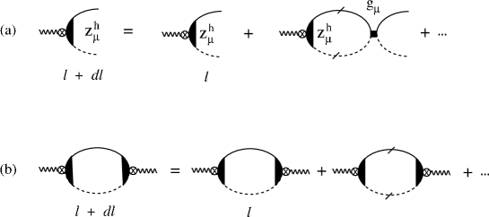
FIGURE 10: Diagrams of the flow equations of the pair vertex part $z_{\mu}^{h}$ (a) and susceptibility $\chi_{\mu}$ (b) in the channel $\mu$.

In the gapless regime for both spin and charge when $g_{1}>0$ and $g_{1}-2g_{2}>\mid g_{3}\mid$, the $\mu=$TS and $\mu=$SS responses are singular

$${\chi}_{\mu}(T)\ \sim\Bigl{(}{T\over E_{F}}\Bigr{)}^{-\gamma^{*}_{\mu}}.$$ (1.150)

Here the exponents $\gamma^{*}_{TS}=\gamma^{*}_{SS}=-g_{2}^{*}-g_{2}^{*2}/2$ are equal and take non universal values on the Tomanaga-Luttinger line where only the attractive $g^{*}_{2}$ coupling remains at $\ell\to\infty$ (here the amplitude of the TS response is larger). Finally, there is a sector of coupling constants, that is when $g_{1}<0$ and $g_{1}-2g_{2}<\mid g_{3}\mid$, where a gap develops in both the spin and charge degrees of freedom. In this sector, BOW (site CDW) is singular for $g_{3}>0$ ($g_{3}<0$) with an exponent larger than 2,[45] which indicates once again that the KW perturbative RG becomes inaccurate in the strong coupling sector. The instabilities of the 1D interacting Fermi systems are summarized in Figure 11.

FIGURE 11: Phase diagram of the 1D interacting Fermi gas in the presence of Umklapp scattering.

Before closing this section we would like to analyze the scaling properties of the two-particle response function. To do so, it is useful to restore the wave vector dependence of $\chi_{\mu}$ by evaluating the upper bound of the loop integral in (1.144) at

$$\ell\to\ell(q,T)=\ln{1.13E_{F}\over T}+\,\psi(1/2)-\frac{1}{2}\Big{[}\psi\Big{(}\,1/2+i{v_{F}q\over 4\pi T}\,\Big{)}+{\rm c.c}\,\Big{]},$$ (1.151)

which coincides with the complete analytical structure of the free Peierls and Cooper loop in (1.47) and (1.50) in the static limit, respectively. At low temperature when $\mid v_{F}q\mid\gg 4\pi T\to 0$, we can use (1.53) and obtain

$$\chi_{\mu}(q)\propto q^{-\gamma_{\mu}}\hskip 28.45274pt{\rm or}\hskip 28.45274pt\chi_{\mu}(x)\propto x^{\gamma_{\mu}-2},$$ (1.152)

which are consistent with the scaling relation $2-\eta_{\mu}=\gamma_{\mu}$ at $\nu=1$ (Eqn. (1.19)).

5 Interchain coupling: one-particle hopping

Let us now consider the effect of a small interchain hopping (Figure 1) in the framework of the KW renormalization group. The bare propagator of the action at $\ell=0$ is then replaced by $G_{p}^{0}({\bf k},\omega_{n})$ given in (1.66). The parameter space for the action at $\ell=0$ then becomes

$$\mu_{S}=(G_{p}^{0}(k,\omega_{n}),t_{\perp},g_{1},g_{2},g_{3}).$$

Now applying the rescaling transformations (1.82-1.83) in the absence of interaction, the rescaling of 1D energy leads to the transformation

$$t^{\prime}_{\perp}=st_{\perp},$$ (1.153)

which means that the canonical dimension of $t_{\perp}$ is unity and it is therefore a relevant perturbation. An estimate of the temperature at which a dimensionality crossover in the coherence of single-particle motion occurs can be obtained by replacing $s$ with the ratio $\xi/a$ and setting $t^{\prime}_{\perp}\sim E_{F}$. We find $T_{x^{1}}\sim t_{\perp}$ in agreement with the results of § 3.2. How this is modified in the presence of interactions will depend on the anomalous dimension $\theta$ which the fermion field acquires under 1D renormalization. When the partial trace is performed at low values of $\ell$, one-particle self-energy corrections are essentially 1D in character and are governed by (1.118). At step $\ell$, the effective 2D propagator then takes the form

$$G^{0}_{p}({\bf k},\omega_{n})=z(\ell)[G^{0-1}_{p}(\widetilde{k})+2t_{\perp}z(\ell)\cos k_{\perp}]^{-1}.$$ (1.154)

Therefore the power law decay of the quasi-particle weight and the density of states (cf. Eqn. (1.135)) along the chains leads to a renormalized hopping amplitude $zt_{\perp}$ which decreases as a function of $\ell$. The condition for the single particle crossover temperature $T_{x^{1}}$ is then renormalized, becoming $z(T)t_{\perp}\xi/a\sim E_{F}$, which implies

$$T_{x^{1}} \sim t_{\perp}\bigl{(}{t_{\perp}\over E_{F}}\bigr{)}^{{1-\theta\over\theta}}$$ (1.155)

$$\propto t_{\perp}^{1/\phi_{x^{1}}},$$ (1.156)

where $\phi_{x^{1}}=1-\theta$ is the single particle crossover exponent. [55, 15] In this simple picture, well below $T_{x^{1}}$, the system behaves as a Fermi liquid. The effective bare propagator (1.154) for $E_{p}({\bf k})<\frac{1}{2}E_{0}(\ell_{x^{1}})$, where $\ell_{x^{1}}=\ln E_{F}/T_{x^{1}}$, has the Fermi liquid form (1.7) with a weight that is consistent with the extended scaling expression (1.23) with $\bar{\gamma}=1-\theta$, $\dot{\bar{\gamma}}=1$ and the non universal constant $z_{\infty}=E_{F}^{\theta/(\theta-1)}$.

As long as $\theta<1$, $t_{\perp}$ remains a relevant variable and $T_{x^{1}}$ is finite. For $\theta=1$ and $\theta>1$, however, it becomes marginal and irrelevant respectively. In these latter cases, transverse band motion has no chance to develop and fermions are confined along the chains at all temperatures. In the KW framework, conditions for 1D single-particle confinement are likely to be realized in the presence of a gap since in this case we have seen that $\theta\sim 1$. [56, 57, 58] Single-particle confinement is also present in the absence of any gaps, as in the Tomanaga-Luttinger model, where $g_{1}=g_{3}=0$ and $\theta\sim 1$ when $\mid g_{2}\mid$ is close to unity [50, 49] and other interacting fermion models [59, 60]. The dependence of the single-particle crossover temperature on the interaction strength, parametrized by the exponent $\theta$, is given in Figure 12.

FIGURE 12: Crossover temperature variation as a function of the one-particle self-energy exponent $\theta$.

A point worth stressing here is that the expression (1.154) for the effective propagator is equivalent to an RPA approach for the interchain motion and is therefore not exact. [61, 62, 63, 64] It becomes exact when interchain single-particle hopping has an infinite range.[61] Another point worth stressing is the fact that the temperature interval over which the single-particle dimensionality crossover takes place is not small. In effect, as already noticed in § 2.1, the critical 1D temperature domain stretches from $E_{F}$ to $T$ making the crossover as a function of temperature gradual.

5.1 Interchain pair hopping and long-range order

Although transverse coherent band motion is absent above $T_{x^{1}}$, a finite probability for fermions to make a jump on neighboring chains still survives within the thermal coherence time $\tau\sim 1/T$. When this “virtual” motion is combined with electron-electron interactions along the stacks, it generates an effective interchain hopping for pairs of particles that are created in all 1D channels of correlations (Peierls, Cooper, and Landau).[14, 37, 15] When coupled with singular pair correlations along the chains, as may occur in the Cooper or Peierls channels, effective transverse two-particle interaction may arise and lead to the occurrence of long-range order above $T_{x^{1}}$, even when fermions are still confined along the chains either by thermal fluctuations or by the presence of a gap. In other words, interchain pair processes generate a different kind of dimensionality crossover, which in turn introduces a new fixed point connected to long-range order. It should be noticed, however, that long-range order is not possible in two dimensions if the order parameter has more than one component.[41] In such a case, a finite coupling in a third direction is required.

To see how these new possibilities emerge from the renormalization group method described above, the quasi-1D propagator (1.154) is used in the evaluation of the one-loop outer shell corrections $\frac{1}{2}\langle S^{2}_{I,2}\rangle_{\bar{0},c}$ and the perturbative influence of $t_{\perp}$ in both Peierls and Cooper channels is shown in Figure 13. The first term is independent of $t_{\perp}$ and reproduces the 1D one-loop corrections. The second diagram expresses the generation at each outer shell integration of an elementary contribution to interchain hopping of a pair of particles in the Peierls or Cooper channel. This outer shell generating term is given by

$$S^{0}_{\perp}[\psi^{\ast},\psi]=-{d\ell\over 2}z^{-2}(\ell)\pi v_{F}\sum_{\mu}\sum_{\widetilde{Q}}f_{\mu}({\bf Q},\ell)O^{\ast}_{\mu}(\widetilde{Q})O_{\mu}(\widetilde{Q}),$$ (1.157)

where ${\bf Q}=(q_{0},q_{\perp}),\widetilde{Q}=(q,q_{\perp},\omega_{m})$ and

$$f_{\mu}({\bf Q},\ell)=\pm 2\Bigl{[}{g_{\mu}(\ell)z(\ell)t_{\perp}\over E_{0}(\ell)}\Bigr{]}^{2}\cos q_{\perp}.$$ (1.158)

The upper (lower) sign refers to the Peierls (Cooper) channel.

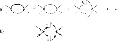
FIGURE 13: a) Generation of interchain pair hopping from one-loop backward and forward vertex corrections in the Cooper and Peierls channels at each outer shell integration. Here the thick (thin) continuous and dashed lines refer to $\pm k_{F}$ 2D (1D) propagator. b) The Umklapp contribution to interchain pair hopping in the Peierls channel.

This term was not present in the bare action and must be added to $\mu_{S}(\ell)$. Furthermore, it will be coupled to other terms of $S$ giving rise to additional corrections and hence to an effective interchain two-particle action of the form

$$S_{\perp}[\psi^{\ast},\psi]=-{1\over 2}z^{-2}(\ell)\sum_{\mu}\sum_{\widetilde{Q}}V_{\mu}({\bf Q},\ell)O^{\ast}_{\mu}(\widetilde{Q})O_{\mu}(\widetilde{Q}),$$ (1.159)

where $V_{\mu}({\bf Q},\ell)$ is the pair tunneling amplitude. As a function of $\ell$, the parameter space of the action then becomes

$$\mu_{S}(\ell)=(zG_{p}^{0},zt_{\perp},z_{1}g_{1},z_{2}g_{2},z_{3}g_{3},V_{\mu},\ldots)$$

Among the most interesting pair tunneling processes in the Peierls channel, $V_{\mu^{+}_{P}\not=0}$ corresponds to an interchain kinetic exchange and promote site SDW or AF ordering (Figure 14), while $V_{\mu^{-}_{P}=0}$ is an interchain BOW coupling which is involved in spin-Peierls ordering. [16] Both favor the transverse propagation of order at ${\bf Q}_{0}=(2k_{F},\pi)$, which actually coincides with the best nesting vector of the whole warped Fermi surface. In the Cooper channel, $V_{\mu_{C}}$ describes the interchain Josephson coupling for SS and TS Cooper pair hopping. According to Figure 11, these terms can only couple to singular intrachain correlations when Umklapp scattering is irrelevant. Long-range order in the Cooper channel is uniform and occurs at the wave vector ${\bf Q}_{0}=(0,0)$.

FIGURE 14: Antiferromagnetic interchain exchange $V_{\mu_{P}^{+}}$ occurring between two spins within the coherence length $\xi$. In the presence of a charge gap, the exchange takes place in the interval $\xi\to\xi_{\rho}\sim v_{F}/\Delta_{\rho}$.

Long-range order will occur at the critical point determined by $\ell_{c}=\ln(E_{F}/T_{c,\mu})$ where $V_{\mu}({\bf Q}_{0},\ell_{c})\rightarrow\infty$. A reasonable way to obtain an approximate $T_{c,\mu}$ is a transverse RPA approach (Fig 15), which consists of treating interchain coupling in the mean-field approximation while the intrachain correlations are taken into account rigorously using (1.148) or the exact asymptotic form of the pair susceptibility when it is known. Thus substituting $S_{I}\rightarrow S_{I}+S_{\perp}$ in (1.89), one gets the one-loop outer-shell contribution ${1\over 2}\langle S^{2}_{I,2}+2S_{I,2}S_{\perp,2}+S^{2}_{\perp,2}\rangle_{\bar{0}}$. The first term leads to the generating term (1.157) to second order in $zt_{\perp}$, whereas the second term introduces pair vertex corrections to the composite field $O_{\mu}^{(*)}$ which can then be expressed in terms of $\bar{\chi}_{\mu}$ given in (1.148). Finally, the third term is the RPA contribution that enables the free propagation of pairs in the transverse direction and hence the possibility of long-range order at finite temperature (Fig. 15). In all cases other than the generating term, the outer-shell integration in the RPA approach is made by neglecting $t_{\perp}$, with the result

$${d\over d\ell}V_{\mu}({\bf Q},\ell)=f_{\mu}+V_{\mu}{d\over d\ell}\ln\bar{\chi}_{\mu}-{1\over 2}(V_{\mu})^{2}$$ (1.160)

for the flow equation of the interchain pair hopping. The solution of this inhomogeneous equation at $\ell$ has the simple pole structure

$$V_{\mu}({\bf Q},\ell)={\bar{V}_{\mu}({\bf Q},\ell)\over 1-{1\over 2}\bigl{(}\bar{\chi}_{\mu}(\ell)\bigr{)}^{-1}\bar{V}_{\mu}({\bf Q},\ell)\chi_{\mu}(\ell)},$$ (1.161)

where

$$\bar{V}_{\mu}({\bf Q},\ell)=\bar{\chi}_{\mu}(\ell)\int^{\ell}_{0} d\ell^{\prime} f_{\mu}({\bf Q},\ell^{\prime})\bigl{(}\bar{\chi}_{\mu}(\ell^{\prime})\bigr{)}^{-1}$$ (1.162)

$$\times \bigl{[}1-{1\over 2}\bigl{(}\bar{\chi}_{\mu}(\ell^{\prime})\bigr{)}^{-1}\bar{V}_{\mu}({\bf Q},\ell^{\prime})\chi_{\mu}(\ell^{\prime})\bigr{]}^{2}.$$ (1.163)

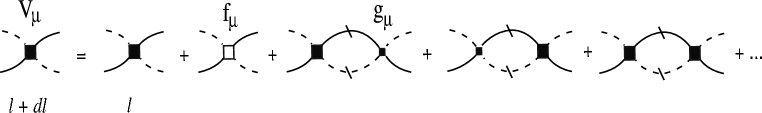
FIGURE 15: Recursion relation for the interchain pair hopping term in the transverse RPA treatment (Eqn.(1.160)).

Critical temperature in the random phase approximation

Owing to the structure of $\bar{V}_{\mu}$, a general analytic solution for $T_{c,\mu}$ is impossible. However, an approximate expression for the critical temperature can be readily obtained, by first neglecting transients in the power laws of $\bar{\chi}_{\mu}\sim e^{\gamma_{\mu}\ell}$, $z\sim e^{-\theta\ell}$, and the couplings $g_{\mu}(\ell)$, and by setting to unity the term in square brackets in the integrand of (1.163). Thus, far from $T_{c,\mu}$ where the RPA term can be neglected, one can write

$$V_{\mu}({\bf Q}_{0},\ell)\approx 2{\langle g^{2}_{\mu}\rangle t^{2}_{\perp}\over E^{2}_{0}}\bigl{(}(2-2\theta-\gamma_{\mu})^{-1}(e^{\ell(2-2\theta-\gamma_{\mu})}-1\bigr{)},$$ (1.164)

where $\langle g_{\mu}^{2}\rangle$ is an average of the coupling constants over the interval $[0,\ell]$. In the presence of a gap in the charge or spin sector, the above scaling form at $\ell\gg\ell_{\nu=\rho,\sigma}=\ln(E_{F}/T_{\sigma,\rho})$ is governed by the strong coupling condition $2-2\theta^{*}-\gamma^{*}_{\mu}<0$ , while for $\ell\ll\ell_{\nu=\rho,\sigma}$, the couplings are weak and $2-2\theta-\gamma_{\mu}>0$. In strong coupling when $\ell\mid 2-2\theta^{*}-\gamma^{*}_{\mu}\mid\gg 1$, the expression (1.164) actually coincides with $\bar{V}_{\mu}$ so that its substitution in (1.161) leads to a non-self-consistent pole at

$$T_{c,\mu}\approx T_{\nu}\bigl{[}{g_{\perp\mu}\over\delta_{\mu}\gamma^{*}_{\mu}}\big{(}1+{g_{\perp\mu}\over\delta_{\mu}\gamma^{*}_{\mu}}\big{)}^{-1}\bigr{]}^{1/\gamma^{*}_{\mu}},$$ (1.165)

where

$$g_{\perp\mu}={\langle g_{\mu}^{2}\rangle z^{2}(\ell_{\nu})\over 2-2\theta-\gamma_{\mu}}{t^{2}_{\perp}\over\Delta^{2}_{\nu}}$$ (1.166)

is an effective interchain pair hopping term at the step $\ell_{\nu}$. This form is reminiscent of a perturbative expansion in terms of the small parameter $zt_{\perp}/\Delta_{\nu}$ indicative of interchain hopping of bound pairs. [65, 66, 67] The positive constant

$$\delta_{\mu}=1+g_{\perp\mu}(\Delta_{\nu}/E_{0})^{\gamma_{\mu}}\chi_{\mu}(\Delta_{\nu})<1$$ (1.167)

corresponds to the integral of $(\ref{Vbar})$ over the interval $[0,\ell_{\nu}]$ at high energy. These results in the presence of a gap allow us to write

$$T_{c,\mu}\sim\ T_{x^{2}}\sim \ g_{\perp\mu}^{1/\phi_{x^{2}}},$$ (1.168)

which is compatible with (1.28) from the extended scaling ansatz. $T_{x^{2}}$ is thus a temperature scale for the dimensionality crossover for the correlation of pairs of particles induced by $g_{\perp\mu}$, and $\phi_{x^{2}}=\gamma_{\mu}^{*}$ is the two-particle exponent.[15] $T_{x^{2}}$ may also be equated with the onset of critical (Gaussian) fluctuations. A point that is worth noticing here concerns the variation of the critical temperature with the gap $\Delta_{\nu}$. Actually, for most interesting situations, the flow of coupling constants will cross the Luther-Emery line and the use of the expression (111) with $\gamma^{*}=1$ will lead to the dependence $T_{c,\mu}\approx z^{2}(\ell_{\nu})t^{2}_{\perp}/\Delta_{\nu}$ in which $T_{c,\mu}$ increases as the amplitude of the gap decreases (Figure 16). In the absence of a gap, the interchain pair hopping term is still present and it can lead to long-range ordering. Sufficiently far from the critical point and for $\ell(2-2\theta-\gamma_{\mu})\gg 1$, one finds

$$V_{\mu}({\bf Q}_{0},\ell) = \bar{V}_{\mu}({\bf Q}_{0},\ell)$$ (1.169)

$$\approx -2g_{\perp\mu}(2-2\theta-\gamma_{\mu})^{-1}(E_{0}(\ell)/E_{0})^{2\theta-2}$$ (1.170)

where in weak coupling $g_{\perp\mu}=\langle g_{\mu}^{2}\rangle t^{2}_{\perp}/E^{2}_{0}$. Substituting this expression for $\bar{V}_{\mu}$ in the RPA expression (1.161), the critical point will occur at

$$T_{c,\mu}\sim E_{F}\bigl{(}g_{\perp\mu}/[\gamma_{\mu}(2-2\theta-\gamma_{\mu})]\bigr{)}^{{1\over 2(1-\theta)}}.$$ (1.171)

Therefore, in weak coupling, $T_{c,\mu}\sim T_{x^{2}}\sim(g_{\perp\mu})^{1/\phi_{x^{2}}}$, and one can define the two-particle crossover exponent $\phi_{x^{2}}=2(1-\theta)$ which is twice $\phi_{x^{1}}$ (plus anomalous corrections coming from the $g_{\mu}$). The critical temperature $T_{c,\mu}\approx\langle g_{\mu}^{2}\rangle^{\frac{1}{2}}\,zt_{\perp}$ will then decrease when interaction decreases. This result is meaningful as long as $T_{x^{2}}>T_{x^{1}}$, that is when the two-particle dimensionality crossover that marks the onset of Gaussian critical fluctuations still falls in a temperature region where the transverse single particle motion is incoherent. The interval of coupling constants where this occurs is relatively narrow, however, since when there is no gap $t_{\perp}$ is a relevant parameter and the calculated $T_{x^{1}}$ increases with decreasing interactions. When the strong and weak coupling regimes are looked at together, a maximum of $T_{c,\mu}$ is therefore expected at the boundary (Figure 16).

Finally, it should be stressed that whenever the strong coupling condition $2-2\theta-\gamma<0$ is achieved in the absence of any gaps as in the case for the Tomanaga-Luttinger model, there is no maximum of $T_{c,\mu}$. Instead, it is found to increase monotonically with the interaction strength (see the dotted line of Figure 16).[61, 66]

Response functions

The calculation of the response functions in the presence of interchain pair hopping can be done following the procedure given in § 4.4. At the RPA level for the pair hopping, one must add the outer-shell contribution $\langle S_{h}S_{\perp,2}\rangle_{\bar{0},c}$ to the scaling equation for $\bar{\chi}_{\mu}$ in the 1D regime (see Eqn. (1.148)), to get

$${d\over d\ell}\ln\bar{\chi}_{\mu}({\bf Q},\ell)={d\over d\ell}\ln\bar{\chi}_{\mu}(\ell)-V_{\mu}.$$ (1.172)

Using (1.161), the integration of this equation leads to

$$\bar{\chi}_{\mu}({\bf Q},\ell)\approx{\bar{\chi}_{\mu}(\ell)\over\big{[}\,1-{1\over 2}\bigl{(}\bar{\chi}_{\mu}(\ell)\bigr{)}^{-1}\bar{V}_{\mu}({\bf Q},\ell)\chi_{\mu}(\ell)\,\big{]}^{2}},$$ (1.173)

which presents a singularity that is quadratic in $(T-T_{c,\mu})^{-1}$ at ${\bf Q}={\bf Q}_{0}$. The exponent $\dot{\gamma}$ (cf. Eqn. (1.26)) for the auxiliary susceptibility is therefore twice the value expected for $\chi_{\mu}$ in the transverse RPA approach. For the cases of two-particle crossovers in § 5.1, this expression at ${\bf Q}_{0}$ can also be written in an extended scaling form similar to (1.27)

$$\bar{\chi}_{\mu}({\bf Q}_{0},\ell)\approx\bar{\chi}_{\mu}({\bf Q}_{0},\ell)X(Bg_{\perp\mu}/T^{\phi_{x^{2}}})$$ (1.174)

where $X(y)=1/(1-y)^{2}$ is the RPA crossover scaling function for the auxiliary susceptibility.

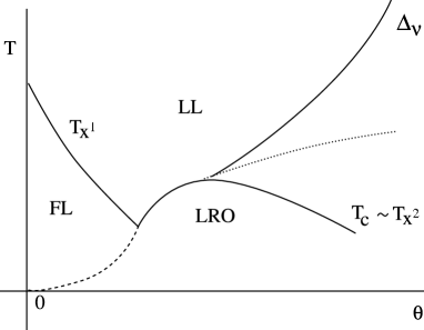
FIGURE 16: Schematic diagram of the temperature ($T$) and interaction strength ($\theta$) dependence of the single-particle and pair dimensionality crossovers from the Luttinger liquid (LL) or Luther-Emery liquid ($T<\Delta_{\nu}$) towards a Fermi liquid (FL) or long-range ordering (LRO). The dashed (dotted) line corresponds to the onset of LRO from a Fermi liquid (gapless LL in strong coupling).

In the present transverse RPA scheme, the small longitudinal $q$ dependence can be incorporated in $\bar{\chi}_{\mu}$ through the substitution (1.151), while the $q_{\perp}$ dependence will come from an expansion of $\bar{V}_{\mu}$ in (1.163) around the transverse ordering wavector $q_{\perp 0}$ in the channel considered. The Q dependence of $\bar{\chi}_{\mu}$ will take the form

$$\bar{\chi}_{\mu}({\bf Q},T)\propto(\dot{t}+\dot{\xi}_{0}^{2}q^{2}+\dot{\xi}_{\perp 0}^{2}q_{\perp}^{2})^{-2}$$ (1.175)

where $\dot{\xi}_{0}\sim v_{F}/T_{c}$ is the longitudinal coherence length; the transverse coherence length $\dot{\xi}_{\perp 0}<1$ is smaller than the interchain distance indicating strong anisotropy. The growth of the correlation length is governed by the usual Gaussian expression $\vec{\dot{\xi}}={\dot{\!\vec{\xi}}_{0}}\,\dot{t}^{-1/2}$, which according to (1.31), leads to the correlation exponent $\dot{\nu}=1/2$. Similar agreement with scaling is found for the response function, for which the above RPA treatment leads to the familiar results $\dot{\gamma}=1$ and $\dot{\eta}=0$.

5.2 Long-range order in the deconfined region

Critical temperatures in the ladder approximation

When the calculated value of $T_{x^{2}}$ becomes smaller than the single-particle deconfinement temperature $T_{x^{1}}$, the two-particle crossover is irrelevant and the expression (1.171) for $T_{c,\mu}$ becomes incorrect. In effect, thermal fluctuations have energies smaller than the characteristic energy related to the warping of the Fermi surface, which then becomes coherent. The $t_{\perp}$ expansion of Fig. 13 stops being convergent and the flow equation (1.160) must be modified accordingly. Now the effective low-energy spectrum

$$E_{p}({\bf k})=\epsilon_{p}(k)-2zt_{\perp}\cos k_{\perp}$$ (1.176)

is characterized by the electron-hole symmetry (nesting) $E_{+}({\bf k}+{\bf Q}_{0})=-E_{-}({\bf k})$ and logarithmic corrections will also be present below $E_{0}(\ell_{x^{1}})$ (Figure 17-a). Similarly in the Cooper channel, the inversion property of the spectrum $E_{+}({\bf k})=E_{-}(-{\bf k})$ also leads to a logarithmic singularity in the same energy range (Figure 17-b). We will follow a simple two-cutoff scaling scheme,[68, 65, 15] in which the flows of $V_{\mu}$ (Eqn. (1.160)) and $g_{\mu}$ (Eqn. (1.128)) are stopped at $\ell_{x^{1}}$ and their values are used as boundary conditions for the outer shell integration below $E_{0}(\ell_{x^{1}})$ which is done with respect to constant warped energy surfaces (Figure 17). The outer shell integration will be done at the one-loop level in the so-called ladder approximation meaning that the interference between the Cooper and Peierls channels will be neglected. This decoupling between the two channels at $T\ll T_{x^{1}}$ is actually not a bad approximation for $T_{c,\mu}$ when the couplings are attractive and favor superconductivity or when the nesting properties of the warped Fermi surface are good and a density-wave instability is expected. The approximation becomes less justified, however, if for example nesting deviations are present in the spectrum and the instability of the Peierls channel is weakened. In this case, it has been shown that the residual interference between the two channels gives rise to non-trivial influence on pairing which becomes non-uniform along the Fermi surface $-$ e.g. unconventional superconductivity for repulsive interactions and anisotropy of the SDW gap.[69]

FIGURE 17: (a) particle-hole pairing in the Peierls channel at ${\bf Q}_{0}=(2k_{F},\pi)$. (b) Particle-particle (or hole-hole) pairing in the Cooper channel. Constant energy surfaces at $\pm\frac{1}{2}E_{0}(\ell>\ell_{x^{1}})$ from the Fermi surface are shown as dashed lines.

In the ladder approximation, the evaluation of $\frac{1}{2}\langle S^{2}_{\perp,2}\rangle_{\bar{0},c}$ at ${\bf Q}_{0}$ in each channel allows us to write

$${dV_{\mu}\over d\ell}=V_{\mu}g_{\mu}-{1\over 2}(V_{\mu})^{2}.$$ (1.177)

This expression is incomplete, however, because ${1\over 2}\langle S^{2}_{I,2}\rangle_{\bar{0},c}$ evaluated at ${\bf Q}_{0}$, gives a logarithmic outer shell correction of the form ${1\over 2}g_{\mu}^{2}d\ell$, which leads to the flow equation

$${dg_{\mu}\over d\ell}={1\over 2}(g_{\mu})^{2}.$$ (1.178)

In the action, the corresponding combination of couplings is proportional to $O^{*}_{\mu}O_{\mu}$, and will then add to $V_{\mu}$. Therefore it is useful to define ${\cal G}_{\mu}\equiv V_{\mu}-g_{\mu}$ for which one obtains the flow equation of Fig. 18

$${d\over d\ell}{\cal G}_{\mu}=-{1\over 2}({\cal G}_{\mu})^{2}.$$ (1.179)

The relevant parameter space for the action for $E_{0}(\ell)<E_{0}(\ell_{x^{1}})$ in the ladder approximation becomes

$$\mu_{S}(\ell>\ell_{x^{1}})=(G^{0}_{p}({\bf k},\omega_{n}),{\cal G}_{\mu}).$$ (1.180)

The solution of (1.179) has the following simple pole structure

$${\cal G}_{\mu}(\ell)={{\cal G}_{\mu}(\ell_{x^{1}})\over 1+{1\over 2}{\cal G}_{\mu}(\ell_{x^{1}})(\ell-\ell_{x^{1}})},$$ (1.181)

where ${\cal G}_{\mu}(\ell_{x^{1}})$ is the boundary condition deduced from the 1D scaling equations (1.160) and (1.128) at $\ell_{x^{1}}$. The presence of an instability of the Fermi liquid towards the condensation of pairs in the channel $\mu$ occurs at the critical temperature

$$T_{c,\mu}=T_{x^{1}}\ \exp\bigl{(}-2/\mid{\cal G}_{\mu}(\ell_{x^{1}})\mid\bigr{)}.$$ (1.182)

This BCS type of instability occurs when the effective coupling constant is attractive (${\cal G}_{\mu}<0$). The phase diagram coincides with the one found in 1D when there is perfect nesting (see Fig. 11). The critical temperature in each sector is associated with those correlations having the largest amplitude. The variation of the critical temperature as a function of the interaction strength is shown by the dashed line in Figure 16. We also notice that the BCS expression (1.182) satisfies the extended scaling hypothesis (1.30), namely $T_{c,\mu}\propto T_{x^{1}}\propto t_{\perp}^{1/\phi_{x^{1}}}$.

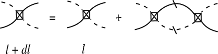
FIGURE 18: Recursion relation in the ladder approximation for the effective coupling ${\cal G}_{\mu}\equiv V_{\mu}-g_{\mu}$ (crossed square) in the channel $\mu$ below the temperature of the single-particle dimensionality crossover $T_{x^{1}}$.

Response functions in the deconfined region

By adding the coupling of fermion pairs to source fields, the calculation of response functions in the channel $\mu$ below $T_{x^{1}}$ can readily be done. In the ladder approximation, the outer shell contraction $\frac{1}{2}\langle S_{h}S_{I,2}\rangle_{\bar{0},c}$, which amounts making the substitution $g_{\mu}\to{\cal G}_{\mu}$ in Fig. 10, leads at once to the flow equation for the pair vertex part

$${d\over d\ell}\ln z_{\mu}^{h}=-\frac{1}{2}{\cal G}_{\mu}.$$ (1.183)

Using the ladder result (1.181), one gets for the auxiliary susceptibility $\bar{\chi}_{\mu}=(z_{\mu}^{h})^{2}$ at $\ell\geq\ell_{x^{1}}$

$$\bar{\chi}_{\mu}({\bf Q}_{0},\ell)={\bar{\chi}_{\mu}({\bf Q}_{0},\ell_{x^{1}})\over[1+\frac{1}{2}{\cal G}_{\mu}(\ell_{x^{1}})(\ell-\ell_{x^{1}})]^{2}},$$ (1.184)

which presents a power law singularity that is quadratic in $(T-T_{c,\mu})^{-1}$ as the temperature approaches $T_{c,\mu}$ from above. The integration of this expression following the definition given in Eqn. (1.144) causes no difficulties and one finds for the response function

$$\chi_{\mu}({\bf Q}_{0},\ell)=\chi_{\mu}({\bf Q}_{0},\ell_{x^{1}})-(\pi v_{F})^{-1}{\chi_{\mu}({\bf Q}_{0},\ell_{x^{1}})(\ell-\ell_{x^{1}})\over 1+\frac{1}{2}{\cal G}_{\mu}(\ell_{x^{1}})(\ell-\ell_{x^{1}})}.$$ (1.185)

The singularity appears in the second term and is linear in $(T-T_{c,\mu})^{-1}$, which is typical of a ladder approximation. The critical exponent defined in Eqn. (1.26) is $\dot{\gamma}=1$ and corresponds to the prediction of mean-field theory. As for the amplitude of the singular behavior, it satisfies the extended scaling constraint shown in (1.29). It is worth noting that these scaling properties are also satisfied by the auxiliary susceptibility.

In going beyond the ladder approximation, the RG technique for fermions becomes less reliable in the treatment of fluctuation effects beyond the Gaussian level which are usually found sufficiently close the critical point $-$ at least in three dimensions. Standard approaches of critical phenomena, such as the statistical mechanics of the order parameter from a Ginzburg-Landau free energy functional, can be used sufficiently close to $T_{c,\mu}$.

6 Kohn-Luttinger mechanism in quasi-one-dimensional metals

6.1 Generation of interchain pairing channels

The outer shell partial integration described in the RPA treatment of § 5.1 for $T>T_{x^{1}}$, namely in the presence of interchain pair hopping, was restricted to the channel $\mu$ corresponding to the most singular correlations of the 1D problem (Figure 11). However, looking more closely at the possible contractions of fermion fields in $S_{\perp,2},$ a new pairing possibility emerges as shown in Figure 19. This consists of putting the two outer-shell fermion fields on separate chains $i$ and $j$, which can then be equated with interchain pairing. The attraction between the two particles in the pair is mediated by the combination of pair hopping and intrachain correlations. Thus interchain pairing is similar to the Kohn-Luttinger mechanism for superconductivity by which Friedel charge oscillations can lead to an effective attraction between two electrons and in turn to an instability of the 3D metal at a finite but extremely low temperature.[33] In quasi-1D systems, however, the K-L mechanism has a dual nature given that interchain pair hopping can exist not only in the Peierls channel but also in the Cooper channel. Therefore for a Josephson coupling, the interchain outer-shell decomposition of Figure 19 leads to an attraction between a particle and hole on different chains. In this case the attraction is mediated by the exchange of Cooper pairs.

Coupling constants

In the following we will restrict our description of the onset of interchain pairing correlations within the KW RG to the incommensurate case where only $g_{1}$ and $g_{2}$ scattering processes are present. Thus in the temperature domain above $T_{x^{1}}$, which corresponds to $\ell<\ell_{x^{1}}$, we have seen in § 5.1 that the outershell contraction in which the fermion lines are diagonal in the chain indices yields the RPA equation (1.160). As pointed out above, another possible contraction would be to put the two outer shell fermion fields on distinct chains.

FIGURE 19: Possible outer-shell contractions for interchain pair hopping: intrachain channel $\mu$ (left) and interchain channel $\bar{\mu}$ (right). The black square corresponds to the pair hopping amplitude $V_{\mu ij}$ between chains $i$ and $j$.

This is best illustrated by first rewriting the pair hopping term (1.159) in terms of chains indices. Then putting two fields in the outershell, we consider the sum of two contributions

$${S}_{\perp,2}+{S^{\prime}}_{\perp,2}= - \,{1\over 2}\pi v_{F}\,z^{-2}(\ell)\sum_{\mu,\tilde{q}}\sum_{i,j}V_{\mu,ij}(\ell)\bigl{(}\bar{O}_{\mu,i}^{*}(\tilde{q})O_{\mu,j}(\tilde{q})+{\rm c.c}\ \bigr{)}$$ (1.186)

$$+ \,{1\over 2}\pi v_{F}\,z^{-2}(\ell)\sum_{\bar{\mu},\tilde{q}}\sum_{i,j}U_{\bar{\mu},ij}(\ell)\bigl{(}\bar{O}_{\bar{\mu},ij}^{*}(\tilde{q})O_{\bar{\mu},ji}(\tilde{q})+{\rm c.c}\ \bigr{)},$$ (1.187)

the first of which leads to (1.160) at the one-loop level, while the second is connected to the interchain channel denoted $\bar{\mu}$. The interchain composite fields are defined by

$$O_{\bar{\mu}_{C},ij}(\tilde{q})=(T/L)^{1/2}\ \sum_{\tilde{k}}\alpha\ \psi_{-,-\alpha,i}(-\tilde{k})\sigma_{\bar{\mu}_{C}}^{\alpha\beta}\psi_{+,\beta,j}(\tilde{k}+\tilde{q})$$ (1.188)

for the singlet (ISS: ${\bar{\mu}_{C}}=0$) and triplet (ITS: ${\bar{\mu}_{C}}=1,2,3$) interchain Cooper channel $\bar{\mu}_{C}$, and by

$$O_{\bar{\mu}_{P},ij}(\tilde{q})=(T/L)^{1/2}\ \sum_{\tilde{k}}\psi^{*}_{-,\alpha,i}(\tilde{k}-\tilde{q})\sigma_{\bar{\mu}_{P}}^{\alpha\beta}\psi_{+,\beta,j}(\tilde{k})$$ (1.189)

for the charge-density-wave (ICDW: ${\bar{\mu}_{P}}=0$) and spin-density-wave (ISDW: ${\bar{\mu}_{P}}=1,2,3$) pair fields of the interchain Peierls channel $\bar{\mu}_{P}$. This introduces the combinations of couplings

$$U_{\bar{\mu},ij}=\sum_{\mu}c_{\mu}^{\bar{\mu}}V_{\mu,ij}.$$ (1.190)

The constants $c_{\mu}^{\bar{\mu}}$ are obtained from

$$U_{\bar{\mu}_{C(P)}=0,ij} = \ {3\over 2}V_{\mu_{P(C)}\neq 0,ij}-{1\over 2}V_{\mu_{P(C)}=0,ij}\hskip 28.45274pt{\rm ISS}\ {\rm(ICDW)}$$ (1.191)

$$U_{\bar{\mu}_{C(P)}\neq 0,ij} = \ {1\over 2}V_{\mu_{P(C)}\neq 0,ij}+{1\over 2}V_{\mu_{P(C)}=0,ij}\hskip 28.45274pt{\rm ITS}\ {\rm(ISDW)}.$$ (1.192)

Therefore at the one-loop level in addition to the RPA term, one obtains the term

$${1\over 2}\langle({S}^{\prime}_{\perp,2})^{2}\rangle_{\bar{0},c}=\ \pi v_{F}z^{-2}(\ell){d\ell\over 4}\sum_{\bar{\mu},\tilde{q}}\sum_{i,j}U^{2}_{\bar{\mu},ij}(\ell)\ O_{\bar{\mu},ij}^{*}(\tilde{q})O_{\bar{\mu},ij}(\tilde{q}),$$ (1.193)

which is also logarithmic. Owing to the dependence on the chain indices of the last composite field on the right hand side of this equation, this term cannot be rewritten in terms of the intrachain channels and therefore stands as a new coupling which we will write $\delta{\cal S}_{\perp}$. It must be added to the parameter space of the action. To do so, it is convenient to recast (1.193) in terms of interchain backward and forward scattering amplitudes:

$$\delta{\cal S}_{\perp}=-{T\over L}\pi v_{F}z^{-2}(\ell)\ d\ell\sum_{\{\alpha\},\tilde{q}}\sum_{i,j} \ \bigl{(}f_{2,ij}(\ell)\delta_{\alpha_{1}\alpha_{4}}\delta_{\alpha_{2}\alpha_{3}}-f_{1,ij}(\ell)\delta_{\alpha_{1}\alpha_{3}}\delta_{\alpha_{2}\alpha_{4}}\bigr{)}$$ (1.194)

$$\times \ \psi^{*}_{+,\alpha_{1},i}(\tilde{k}_{1}+\tilde{q})\psi^{*}_{-,\alpha_{2},j}(\tilde{k}_{2}-\tilde{q})\psi_{-,\alpha_{3},j}(\tilde{k}_{2})\psi_{+,\alpha_{4},i}(\tilde{k}_{1}).$$ (1.195)

The outer-shell backscattering amplitude $f_{1,ij}$ then corresponds to intrachain momentum transfer near $2k_{F}$ between the particles and a change in the chain indices during the process, whereas the forward generating amplitude $f_{2,ij}$ corresponds to small intrachain momentum with no change in the chain index (Figure 20). The explicit expressions are

$$f_{1,ij} = -{1\over 2}[V^{2}_{\mu_{P}\neq 0,ij}-V_{\mu_{P}\neq 0,ij}V_{\mu_{P}=0,ij}]+{1\over 2}[V^{2}_{\mu_{C}\neq 0,ij}-V_{\mu_{C}\neq 0,ij}V_{\mu_{C}=0,ij}]$$ (1.196)

$$2f_{2,ij}-f_{1,ij} = \ \ {1\over 4}[3V^{2}_{\mu_{C}\neq 0,ij}+V^{2}_{\mu_{C}=0,ij}]+{1\over 4}[3V^{2}_{\mu_{C}\neq 0,ij}+V^{2}_{\mu_{P}=0,ij}].$$ (1.198)

Since the pair hopping amplitudes $V_{\mu}$ are themselves generated as a function of $\ell$, it is clear that the $f^{\prime}s$ will be very small except when the $V_{\mu}$ approach the strong coupling regime. Successive KW transformations will lead to the renormalization of the above interchain backward and forward scattering amplitudes which we denote $g_{1,ij}^{\perp}$ and $g_{2,ij}^{\perp}$, respectively. These define the part of the action denoted ${\cal S}_{\perp}$, which when expressed in terms of uniform charge and spin fields introduced in (1.107), takes the rotationally invariant form

$${\cal S}_{\perp}[\psi^{*},\psi]_{\ell}=-\pi v_{F}z^{-2}(\ell)\sum_{p,\tilde{q}}\sum_{ij}\ \Bigl{(}\ (2g^{\perp}_{2,ij}(\ell)-g^{\perp}_{1,ij}(\ell))\ \rho_{p,i}(\tilde{q})\rho_{-p,j}(-\tilde{q})-\ g^{\perp}_{1,ij}(\ell)\ {\bf S}_{p,i}(\tilde{q})\cdot{\bf S}_{-p,j}(-\tilde{q})\ \Bigr{)}$$ (1.199)

This expression clearly shows that interchain pair hopping generates a coupling between uniform charge and spin excitations of different chains. The flow equations of these couplings will now be obtained from ${1\over 2}\langle{\cal S}_{\perp,2}^{2}\rangle_{\bar{0},c}$ at the one-loop level. Aside from the scale dependent generating terms, the contributions consist of the same type of interfering Cooper and Peierls diagrams found in the purely one-dimensional problem (Fig. 5). These outer shell logarithmic contributions can be evaluated at once resulting in the following flow equations for the interchain spin and charge variables

$${d\over d\ell}g_{1,ij}^{\perp} = f_{1,ij}-(g_{1,ij}^{\perp})^{2}$$ (1.200)

$${d\over d\ell}2g_{2,ij}^{\perp}-g_{1,ij}^{\perp} = 2f_{2,ij}^{\perp}-f_{1,ij}^{\perp}.$$ (1.201)

It is interesting to note that, following the example of the purely one-dimensional couplings, the interference between the interchain and Cooper channels causes these equations to be decoupled. Hence the spin and charge degrees of freedom on different chains are not mixed through $g_{1}^{\perp}$ and $g_{2}^{\perp}$.

FIGURE 20: Perpendicular backward ($g_{1}^{\perp}$) and and forward ($g_{2}^{\perp}$) scattering terms generated by interchain pair tunneling.

The solution for the charge coupling is straightforward and one obtains a parquet-type solution for the spin part

$$g_{1,ij}^{\perp}(\ell)={\bar{g}_{1,ij}^{\perp}(\ell)\over 1+\bar{g}_{1,ij}^{\perp}(\ell)\ell}\ ,$$ (1.202)

where

$$\bar{g}_{1,ij}^{\perp}(\ell)=\ \int_{0}^{\ell}d\ell^{\prime}f_{1,ij}(\ell^{\prime})[1+\bar{g}^{\perp}_{1,ij}(\ell^{\prime})]^{2}.$$ (1.203)

According to (1.198), $f_{1,ij}(\ell^{\prime})$ and therefore $\bar{g}_{1,ij}^{\perp}(\ell)$ are negative in the repulsive sector ($g_{1}>0$ and $2g_{2}-g_{1}>0$) where SDW correlations are singular (Figure 11); $g_{1,ij}^{\perp}(\ell)$ has then the possibility to flow to the strong attractive coupling sector indicating the existence of a spin gap. Given the place held by $g_{1,ij}^{\perp}(\ell)$ in the hierarchy of generated couplings of the RG transformation, however, this can only occur if the the SDW pair tunneling or exchange term $V_{\mu_{P}\neq 0,ij}$ first reaches the strong coupling domain $-$ a possibility realized as the system enters the Gaussian critical domain near $T_{x^{2}}$. Since the above flow equations (1.201) hold for all pairs of chains $i$$j$ for $\ell<\ell_{x^{1}}$, the amplitude of the spin gap goes to zero as the separation $|i-j|\to\infty$. It is worth noting that the spin gap for nearest-neighbor chains is reminiscent of the one occurring in the two-chain problem.[70, 71]

Interchain response functions

To establish the nature of correlations introduced by interchain pairing, it is convenient to express outershell decomposition of $S_{\perp}+{\cal S}_{\perp}$ in the corresponding channel

$$S_{\perp,2}+{\cal S}_{\perp,2}\,\Big{|}_{\bar{\mu}^{\pm}}={1\over 2}\pi v_{F}z^{-2}\sum_{\tilde{q},\bar{\mu}^{\pm}}\sum_{ij}\ g^{\perp}_{\bar{\mu}^{\pm},ij}(\ell)\bar{{\cal O}}^{*}_{\bar{\mu}^{\pm},ij}(\tilde{q}){\cal O}_{\bar{\mu}^{\pm},ij}(\tilde{q})+{\rm c.c},$$ (1.204)

where we have introduced the combinations of couplings

$$g^{\perp}_{{\rm ISS}^{\pm},ij} = -g^{\perp}_{1,ij}-g^{\perp}_{2,ij}\pm U_{{\rm ISS},ij}$$ (1.205)

$$g^{\perp}_{{\rm ITS}^{\pm},ij} = \ g^{\perp}_{1,ij}-g^{\perp}_{2,ij}\pm U_{{\rm ITS},ij}$$ (1.206)

for symmetric $(+)$ and antisymmetric $(-)$ interchain superconductivity and their analog expressions

$$g^{\perp}_{{\rm ICDW}^{\pm},ij} = g^{\perp}_{2,ij}-2g^{\perp}_{1,ij}\pm U_{{\rm ICDW},ij}$$ (1.207)

$$g^{\perp}_{{\rm ISDW}^{\pm},ij} = g^{\perp}_{2,ij}\pm U_{{\rm ISDW},ij}$$ (1.208)

for interchain density-wave. The corresponding pair fields are given by

$${\cal O}_{\bar{\mu}^{\pm},ij}={1\over 2}\bigl{(}O_{\bar{\mu},ij}\pm O_{\bar{\mu},ji}\bigr{)}$$ (1.209)

for symmetric $(+)$ and antisymmetric $(-)$ composite fields.

We add the coupling to source fields $S_{h}=\sum O^{*}_{\bar{\mu}^{\pm},ij}h_{\bar{\mu}^{\pm},ij}+{\rm c.c.}$. The one-loop corrections to the pair vertex part are obtained from $\langle(S_{\perp,2}+{\cal S}_{\perp,2}){S}_{h}\rangle_{\bar{0},c}$ (which is equivalent to making the substitution $g_{\mu}\to g^{\perp}_{{\rm ISS}^{\pm},ij}$ in Fig. 10), and yields the flow equations pair vertex renormalization factor $z_{\bar{\mu}^{\pm},ij}$ and hence that of the auxiliary susceptibility $\bar{\chi}_{\bar{\mu}^{\pm},ij}=z_{\bar{\mu}^{\pm},ij}^{2}$ (with $z=1$ ):

$${d\over d\ell}\ln\bar{\chi}_{\bar{\mu}^{\pm},ij}=g^{\perp}_{\bar{\mu}^{\pm},ij}.$$ (1.210)

Obtaining an expression for $\bar{\chi}_{\bar{\mu}^{\pm},ij}$ in closed form for arbitrary chains $i$ and $j$ is not possible. However, in the case where intrachain channels have developed only short-range order and $U_{\bar{\mu},ij}$ is only sizable for nearest-neighbour chains, one can extract the dominant trend of interchain auxiliary suceptibilities in the various sectors of the $g_{1}g_{2}$ plane. Thus by taking in Fourier space $V_{\mu}({\bf Q},\ell)\approx(-1)^{\delta_{\mu\mu_{c}}}\mid V_{\mu}(\ell)\mid\cos q_{\perp}$ for the pair tunneling term (1.161), one gets $V_{\mu,ij}(\ell)={1\over 2}(-1)^{\delta_{\mu\mu_{c}}}\mid V_{\mu}(\ell)\mid$ where $\mid V_{\mu}(\ell)\mid=\mid V_{\mu}({\bf Q}_{0},\ell)\mid$ is the maximum amplitude of $V_{\mu}({\bf Q},\ell)$. This approximation holds sufficiently far from $T_{c,\mu}$, namely for ${1\over 2}\bar{V}_{\mu}\chi_{\mu}/\bar{\chi}_{\mu}$ not too close to unity. The nearest-neighbour $ij$ auxiliary susceptibility then becomes

$$\bar{\chi}_{\bar{\mu}^{\pm},ij}(\ell) = X_{\bar{\mu},ij}(\ell)\exp\left\{\pm{1\over 2}\sum_{\mu}\int_{0}^{\ell}c_{\mu}^{\bar{\mu}}\mid V_{\mu}(\ell^{\prime})\mid d\ell^{\prime}\right\}$$ (1.211)

$$\approx X_{\bar{\mu},ij}(\ell)\prod_{\mu}\Bigl{[}1-{1\over 2}(\bar{\chi}_{\mu}(\ell))^{-1}\bar{V}_{\mu}(\ell)\chi_{\mu}(\ell)\Bigr{]}^{\mp c_{\mu}^{\bar{\mu}}},$$ (1.212)

where the values of the channel index $\mu$ and the exponent $c_{\mu}^{\bar{\mu}}$ are given in (1.190-1.192). The transient amplitude is given by

$$X_{\bar{\mu},ij}(\ell)=\ \exp\left\{\int_{0}^{\ell}\beta_{\bar{\mu}}d\ell^{\prime}\right\},$$ (1.213)

where for superconductivity $\beta_{\rm ISS}=-g^{\perp}_{1,ij}-g^{\perp}_{2,ij}$ and $\beta_{\rm ITS}=g^{\perp}_{1,ij}-g^{\perp}_{2,ij}$, while for density-wave $\beta_{\rm ICDW}=g^{\perp}_{2,ij}-2g^{\perp}_{1,ij}$ and $\beta_{\rm ISDW}=g^{\perp}_{2,ij}$. The onset of interchain correlations, even though they are small, will be essentially determined by the most singular correlations of the intrachain channels $\mu$ (Figure 21) and the exponent $c_{\mu}^{\bar{\mu}}$. At finite temperature, we can write

$$\bar{\chi}_{\bar{\mu}^{\pm},ij}(T)\approx X_{\bar{\mu},ij}(T)\prod_{\mu}\ \Bigl{[}1-{1\over 2}(\bar{\chi}_{\mu}(T))^{-1}\bar{V}_{\mu}(T)\chi_{\mu}(T)\Bigr{]}^{\mp c_{\mu}^{\bar{\mu}}}.$$ (1.214)

In the repulsive sector where $g_{1}>0,2g_{2}-g_{1}>0$, SDW correlations are singular (region I, Figure 21) and lead to an enhancement of symmetric (+) interchain singlet superconducting (ISS⁺) correlations with $c_{\mu_{P}\neq 0}^{\bar{\mu}_{C}=0}=3/2$. It should be noted here that, in this sector, symmetric interchain triplet (ITS⁺) correlations are also enhanced by SDW correlations with $c_{\mu_{P}\neq 0}^{\bar{\mu}_{C}\neq 0}=1/2$. The pairing on different chains results from the exchange of spin fluctuations. On the T-L line at $g_{1}=0$ and $g_{2}>0$, SDW and CDW correlations are equally singular leading to an enhancement of both ISS⁺ and ITS⁺ correlations with a net exponent of unity.

FIGURE 21: Phase diagram of the quasi-one-dimensional electron gas with interchain hopping and no Umklapp scattering. Dominant correlations of intrachain (interchain) pairing channels are given.

In region II of Figure 21, where $g_{1}>0$, $2g_{2}-g_{1}<0$, the TS channel is the most singularly enhanced leading to interchain charge-density-wave (ICDW^-) correlations with $c_{\mu_{P}\neq 0}^{\bar{\mu}_{P}=0}=3/2$. Here the pairing results from a three-component (triplet) Cooper pair exchange between the chains. In the same region, an enhancement, although smaller, of antisymmetric interchain spin-density-wave correlations (ISDW^-) is also present with $c_{\mu_{P}\neq 0}^{\bar{\mu}_{P}\neq 0}=1/2$. On the T-L line at $g_{2}<0$, however, SS and TS are equally singular so both contribute to give the same enhancement for ISDW^- and ICDW^-. If one moves to the attractive sector (region III, Figure 21), where $g_{1}<0$, $2g_{2}-g_{1}<0$ and SS is the most singular channel along the chains, one finds that symmetric ICDW⁺ and antisymmetric ISDW^- channels have similar enhancements $c_{\mu_{C}=0}^{\bar{\mu}_{P}=0}=c_{\mu_{C}=0}^{\bar{\mu}_{P}\neq 0}=1/2$. Finally in the region IV, where $g_{1}<0$, $2g_{2}-g_{1}>0$ and CDW correlations are the most singular, symmetric ITS⁺ correlations are enhanced in the interchain triplet channel with the exponent $c_{\mu_{P}=0}^{\bar{\mu}_{C}\neq 0}=1/2$.

6.2 Possibility of long-range order in the interchain pairing channels

If the initial parameters of the model are such that the system can reach the energy or temperature domain $T_{x^{1}}$ without developing long-range order, the pair-hopping amplitude $V_{\mu}$ is still in the weak coupling regime. We have seen in §5.2, however, that infrared singularities in both the Peierls and Cooper channels persist above $\ell_{x^{1}}$ so that long-range order in the intrachain channel $\mu$ can occur if ${\cal G}_{\mu}<0$. This will be so in the Peierls channel when deviations from perfect nesting of the warped Fermi surface do not exceed a given threshold (Fig. 17-a), while in the Cooper channel if a magnetic field is below a critical value. Therefore sufficiently large nesting deviations or magnetic field must be introduced in the model in order for long-range order in the interchain channels to be possible. We will now illustrate how such a possibility can be realized in the repulsive case when nesting deviations are introduced in the model. We will thus focus our attention in the region I of the phase diagram where symmetric interchain singlet superconductivity (ISS⁺) can be stabilized (Fig. 21). A similar description holds for the Peierls interchain channel in the presence of a sufficiently strong magnetic field (regions II and III in Fig. 21).

Frustration of nesting is commonly introduced by considering the possibility of particles hopping to second nearest-neighbor chains, i.e. by adding the term $-2t_{\perp 2}\cos 2k_{\perp}$ to the spectrum at $\ell=0$, where $t_{\perp 2}$ is the amplitude of the hopping ($t_{\perp 2}\ll t_{\perp}$). The relevant parameter space of the action at the crossover value $\ell_{x^{1}}$ becomes $\mu_{S}(\ell_{x^{1}})=(G_{p}^{0}({\bf k},\omega_{n}),{\cal G}_{\mu},g^{\perp}_{\bar{\mu}^{\pm}})$, where

$$G_{p}^{0}({\bf k},\omega_{n})={z\over i\omega_{n}-\epsilon_{p}(k)+2t^{*}_{\perp}\cos k_{\perp}+2t^{*}_{\perp 2}\cos 2k_{\perp}}$$ (1.215)

is the effective propagator in which $z$ is the quasi-particle weight at $\ell_{x^{1}}$ and $t_{\perp(2)}^{*}\equiv zt_{\perp(2)}$. If one cranks up the amplitude of $t_{\perp 2}^{*}$, nesting of the Fermi surface at ${\bf Q}_{0}=(2k_{F},\pi)$ is quickly suppressed so that the $T_{\rm c,SDW}$ in the region I of the phase diagram decreases rapidly and eventually vanishes above the critical $t^{*c}_{\perp 2}$[72]. As for the infrared singularity of the Cooper channel, however, it is still present and can then lead to an instability of the normal state.

We will adopt here a simple ladder RG description of this instability, which neglects the interference between the $-$ weakened $-$ Peierls channel and the Cooper one. This approximation should be qualitatively valid for $t_{\perp 2}^{*}\gg t^{*c}_{\perp 2}$ (a more quantitative description including the interference effect can be found in Ref. [69]). We will further assume for simplicity that the enhancement of ${\cal G}_{\mu}$ above $\ell_{x^{1}}$ is negligible and the transverse short-range order of the chains is entirely contained in the $ij$ dependence of $g^{\perp}_{{\rm ISS}^{+},ij}$ in Eqns. (1.206) and (1.192), which is restricted to nearest-neighbor chains. In this way, the repulsive coupling ${\cal G}_{\mu}$ is entirely local and does not compete with the interchain part: fermions on different chains are said to avoid intrachain repulsion.[34, 36] In transverse Fourier space, the outer shell decomposition (1.204) in the channel ISS⁺ becomes

$$S_{\perp,2}+{\cal S}_{\perp,2}\,\Big{|}_{{\rm ISS}^{+}}={1\over 2}\pi v_{F}z^{-2}\sum_{\tilde{q}}\sum_{k_{\perp},k^{\prime}_{\perp}}\ g^{\perp}_{{\rm SS}}(\ell)\,{\eta_{k_{\perp}}}\bar{O}^{*}_{{\rm SS}}(\tilde{q},k_{\perp}){\eta_{k^{\prime}_{\perp}}}{O}_{{\rm SS}}(\tilde{q},k^{\prime}_{\perp})+{\rm c.c}$$ (1.216)

in which we have defined ${O}_{{\rm SS}}(\tilde{q})=\sum_{k_{\perp}}{O}_{{\rm SS}}(\tilde{q},k_{\perp})$ and where $\eta_{k_{\perp}}=\cos k_{\perp}$ is the Fourier factor that leads to a global antisymmetric order parameter for interchain singlet superconductivity. The combination of couplings at $\ell$

$$g^{\perp}_{{\rm ISS}^{+}}(\ell)\equiv-g^{\perp}_{1}(\ell)-g^{\perp}_{2}(\ell)+U_{{\rm ISS}}(\ell)$$ (1.217)

is obtained from the amplitude of the transverse couplings at $\ell$. In the ladder approximation, the outer shell integration $\frac{1}{2}\langle(S_{\perp,2}+{\cal S}_{\perp,2})^{2}\rangle_{\bar{0},c}$ is done in this channel. At zero external pair momentum, this leads to the flow equation

$${d\over d\ell}g^{\perp}_{{\rm ISS}^{+}}={1\over 4}(g^{\perp}_{{\rm ISS}^{+}})^{2},$$ (1.218)

which is easily integrated to give the simple pole expression

$$g^{\perp}_{{\rm ISS}^{+}}(\ell)={g^{\perp}_{{\rm ISS}^{+}}(\ell_{x^{1}})\over 1-{1\over 4}g^{\perp}_{{\rm ISS}^{+}}(\ell_{x^{1}})(\ell-\ell_{x^{1}})}.$$ (1.219)

The critical temperature for the superconducting instability is then $T_{c}=T_{x^{1}}\exp[-4/g^{\perp}_{{\rm ISS}^{+}}(\ell_{x^{1}})]$ where $g^{\perp}_{{\rm ISS}^{+}}(\ell_{x^{1}})>0$ corresponds to a net attraction in the interchain superconducting channel. From (1.216), the singlet order parameter is of the form

$$\Delta(k_{\perp})=\Delta_{0}\eta_{k_{\perp}},$$ (1.220)

which has nodes on the Fermi surface.

The calculation of the interchain superconducting response causes no particular difficulty. In effect, by adding the coupling to a source field ($S_{h}=\sum{{O}}^{*}_{\bar{\mu}^{+}}(\widetilde{q},k_{\perp})\eta_{k_{\perp}}h_{\bar{\mu}^{+}}+{\rm c.c.}$), one obtains the flow equation for the auxiliary susceptibility

$${d\over d\ell}\ln\bar{\chi}_{{\rm ISS}^{+}}=\frac{1}{2}g^{\perp}_{{\rm ISS}^{+}}.$$ (1.221)

Using (1.219), this is integrated to give the double pole singularity

$$\bar{\chi}_{{\rm ISS}^{+}}(\ell)={\bar{\chi}_{{\rm ISS}^{+}}(\ell_{x^{1}})\over[1-{1\over 4}g^{\perp}_{{\rm ISS}^{+}}(\ell_{x^{1}})(\ell-\ell_{x^{1}})]^{2}},$$ (1.222)

where the boundary condition $\bar{\chi}_{{\rm ISS}^{+}}(\ell_{x^{1}})$ is given by the solution of (1.210) at $\ell_{x^{1}}$. The loop integration of the above expression following the definition (1.144), leads to the response function

$$\chi_{{\rm ISS}^{+}}(\ell)=\chi_{{\rm ISS}^{+}}(\ell_{x^{1}})-(2\pi v_{F})^{-1}{\bar{\chi}_{{\rm ISS}^{+}}(\ell_{x^{1}})(\ell-\ell_{x^{1}})\over 1-{1\over 4}g^{\perp}_{{\rm ISS}^{+}}(\ell_{x^{1}})(\ell-\ell_{x^{1}})}$$ (1.223)

which has the expected simple pole structure of the ladder approximation.

7 Summary and concluding remarks

We have reexamined the scaling tools that enter in the description of quasi-one-dimensional interacting fermion systems. On phenomenological grounds, we have emphasized that the scaling ansatz can provide a qualitative understanding of the existence of power law behavior of various quantities in one dimension while its extension for non zero interchain coupling has allowed us to describe the different forms of dimensionality crossover in the quasi-one-dimensional case. A key feature of this phenomenology is the existence of fluctuations of single fermion and pair degrees of freedom on many length or energy scales, the origin of which can be microscopically understood using the renormalization group language. We found it useful to reconsider the formulation of this methodology and we have seen that the adoption of a classical Wilson procedure for the Kadanoff transformation has a molding influence on the RG flow beyond the one-loop level. Thus the constraint of a sharp natural cutoff $k_{0}$ on the fermion spectrum which keeps the loop momenta in the outer energy shells inevitably leads to a non-local flow of the parameters that define the action. Non-locality results from the inclusion of many-particle marginal interactions in the outer shell integration. These are not present in the bare action but are generated along the RG flow. The resulting structure of outer shell integration finds an interesting parallel with the functional description of the renormalization group equations proposed by Polchinski in the framework of the $\phi^{4}$ theory,[73] and used by Zanchi and Schulz in the context of two-dimensional interacting fermion systems.[20]

It is only when the marginally relevant or irrelevant couplings are treated in the local approximation that purely logarithmic scaling is recovered. Although this has only been verified at the two-loop loop level and in the one-dimensional case, similar conclusions are expected to hold at higher order and in higher dimensions as well. The procedure described in this review casts light on a previous alternative formulation of the RG which is known to offer a more direct route to logarithmic scaling at high order but which on the other hand requires the relaxation of some of the standard rules of the Wilson method. It also highlights how the difficulties linked to non-locality of the flow equations are essentially hidden in older versions of the renormalization group.

The RG method is widely recognized as a tool well suited to the study of the influence of interchain hopping on the stability of the Luttinger and Luther-Emery liquid states in one dimension. We have reviewed the conditions under which the coupling between stacks can make these non-Fermi liquid states unstable. A possible instability occurs when the Luttinger liquid yields to the formation of a Fermi liquid. The recovery of quasi-particle excitations, here called a dimensionality crossover for the fermion quantum coherence, squares well with the picture provided by the extended scaling ansatz. A second instability emerges when the kinematics of interchain single-particle hopping is combined with intrachain pair correlations. Effective pair hopping processes between chains then form and their coupling to singular correlations along the chains lead to a distinct (two-particle) dimensionality crossover. This is physically meaningful as long as the corresponding temperature scale is above the one predicted for single particles. Such a situation is favored by cranking up interactions which on the one hand increases pair correlations and on the other hand reduces single particle coherence. The temperature scale for two-particle dimensionality crossover marks the onset of long-range order which accords well with the extended scaling ansatz. For sufficiently weak interactions, however, single-particle deconfinement occurs first and the possibility for long-range order remains as an instability of the Fermi liquid. In this case, the ladder level of the RG gives a BCS character to the transition.

The RG method can also be useful in studying how the Kohn-Luttinger mechanism for unconventional pairing works in the quasi-one-dimensional case. We have seen that this mechanism opens up channels of correlation which pair particles on different stacks as a result of pair hopping processes between chains. Since these are present in both the Peierls and Cooper channels, the Kohn-Luttinger mechanism has a dual nature. Thus it was shown not only that the exchange of density-wave correlations can lead to interchain Cooper pairing but also that interchain Peierls pairing between a particle and a hole is also possible when both particles exchange Cooper pairs. Long-range order in these unconventional channels can only be achieved from the Fermi liquid state in which enough nesting deviations or magnetic field are present to frustrate the formation of long-range order in the the primary channels of correlation along the chains.

The results presented in this review by no means exhaust the range of possibilities supplied by the RG method. We will end this article by giving two specific examples. The first concerns the issue of single-particle deconfinement that leads to the recovery of a Fermi liquid. This question is of great interest especially in connection with the normal state properties obeserved in concrete realizations of quasi-one-dimensional materials like the organic conductors.[18, 64] We have seen that the critical domain of the primary (Luttinger liquid) fixed point in a quasi-one-dimensional system essentially covers the whole temperature range of interest. This favors in turn a slow and gradual crossover to a Fermi liquid, which means in practice that transitory effects are likely to be important in the description of these materials. Although crossover scaling effects have been underestimated in the treatment given above, they are not beyond the reach of the RG method.

Another promising avenue is the application of the RG method to interacting fermions on a lattice.[74] The Kadanoff transformation can actually be generalized to fermions with the full tight binding spectrum. Transients to the continuum limit can then be considered in a quantitative way. In the case of the fermion representation of the one-dimensional spin chain, for example, this has been shown to be an essential ingredient in the description of the thermodynamics.

8 Acknowledgements

C.B. thanks L. G. Caron, N. Dupuis, A.-M. Tremblay and D. Sénéchal for numerous discussions and R. Shankar and G. Kotliar for interesting comments about the RG method at high order. This work is supported by the Natural Sciences and Engineering Research Council of Canada (NSERC), le Fonds pour la Formation de Chercheurs et l’Aide à la Recherche du Gouvernement du Québec (FCAR), and by the ‘superconductivity program’ of the Institut Canadien de Recherches Avancées (CIAR).

1 One-particle self-energy at the two-loop level

1.1 Backward and forward scattering contributions

Following the partial trace operation in the absence of umklapp scattering, three-particle interactions are generated from the outer shell contraction $\delta S_{\lambda}^{(j)}\equiv\frac{1}{2}\langle S_{I,1}^{2}\rangle_{\bar{0},c}$. The corresponding expression reads

$$\delta S^{(j)}_{\lambda}=\ (\pi v_{F})^{2}{T^{2}\over L^{2}}\ \sum_{\{\alpha,\alpha^{\prime}\}}\sum_{\widetilde{k}_{1,2},\widetilde{k}^{\prime}_{2},\widetilde{q}^{\prime}}\mathop{\sum\kern-13.99995pt-\kern 5.0pt}_{\widetilde{q}}\lambda^{+}_{\{\alpha,\alpha^{\prime}\}}(\ell_{j-3})G^{0}_{+}(\widetilde{k}_{1}+\widetilde{q}) \!\!\!\!\!\!\!\psi^{*}_{+,\alpha^{\prime}_{1}}(\widetilde{k}_{1}+\widetilde{q}^{\prime}+\widetilde{q})\psi^{*}_{-,\alpha^{\prime}_{2}}(\widetilde{k}^{\prime}_{2}-\widetilde{q}^{\prime})\psi^{*}_{-,\alpha_{2}}(\widetilde{k}_{2}-\widetilde{q})$$ (224)

$$\times \psi_{-,\alpha^{\prime}_{3}}(\widetilde{k}^{\prime}_{2})\psi_{-,\alpha_{3}}(\widetilde{k}_{2})\psi_{+,\alpha_{4}}(\widetilde{k}_{1})$$ (225)

$$+\ (\pi v_{F})^{2}{T^{2}\over L^{2}}\ \sum_{\{\alpha,\alpha^{\prime}\}}\sum_{\widetilde{k}_{1},\widetilde{k}^{\prime}_{1,2},\widetilde{q}^{\prime}}\mathop{\sum\kern-13.99995pt-\kern 5.0pt}_{\widetilde{q}}\lambda^{-}_{\{\alpha,\alpha^{\prime}\}}(\ell_{j-3})G^{0}_{-}(\widetilde{k}_{2}-\widetilde{q}) \!\!\!\!\!\!\!\psi^{*}_{-,\alpha^{\prime}_{2}}(\widetilde{k}^{\prime}_{2}-\widetilde{q}^{\prime})\psi^{*}_{+,\alpha^{\prime}_{1}}(\widetilde{k}^{\prime}_{1}+\widetilde{q}^{\prime})\psi^{*}_{+,\alpha_{1}}(\widetilde{k}_{1}+\widetilde{q})$$ (226)

$$\times \psi_{+,\alpha^{\prime}_{4}}(\widetilde{k}^{\prime}_{1})\psi_{+,\alpha_{4}}(\widetilde{k}_{1})\psi_{-,\alpha_{3}}(\widetilde{k}_{2})$$ (227)

where $\lambda^{+}_{\{\alpha,\alpha^{\prime}\}}(\ell_{j-3})=g_{\{\alpha\}}(\ell_{j-3})g_{\{\alpha^{\prime}\}}(\ell_{j-3})\delta_{\alpha_{1}\alpha^{\prime}_{4}}$, $\lambda^{-}_{\{\alpha,\alpha^{\prime}\}}(\ell_{j-3})=g_{\{\alpha\}}(\ell_{j-3})g_{\{\alpha^{\prime}\}}(\ell_{j-3})\delta_{\alpha_{2}\alpha^{\prime}_{3}}$, $\ell_{j-3}=\ln(E_{0}/E_{0}(\ell_{j-3}))$ and $g_{\{\alpha\}}$ is given by (1.74). Here the summation $\mathop{\sum\kern-11.99998pt-\kern 5.0pt}_{\widetilde{q}}$ covers all $\omega_{m}$ but $q$ is restricted such that $k_{1}+q$ ($k_{2}-q)$ in the propagator $G_{+}^{0}$ ($G_{-}^{0}$) is in the outer momentum shell at the step $(j-2)d\ell$ for $j\geq 3$. The two terms in (227), which depends on the step $j$, correspond to the diagrams of Figure 8-a. At the next partial integration $(j-1)d\ell$ , the above contributions will in turn be contracted leading to a second fermion line at the adjacent momentum shell (Figure 8-b). When this set of contractions is repeated as a function of $j$, contributions add to give an effective two-particle interaction of the form

$$\delta S^{\prime}_{\lambda}\equiv \sum_{j=3}^{N-1}\langle\delta S^{(j)}_{\lambda,2}\rangle_{\bar{0},c}$$ (228)

$$= (\pi v_{F})^{2}{T^{2}\over L^{2}}\sum_{\widetilde{k},\widetilde{q}^{\prime}}\sum_{j=3}^{N-1}\sum_{\{\alpha,\alpha^{\prime}\}}\mathop{\sum\kern-13.99995pt-\kern 5.0pt}_{\widetilde{k}^{\prime}}\!\!{}^{{}^{*}}\ \mathop{\sum\kern-13.99995pt-\kern 5.0pt}_{\widetilde{q}}\lambda^{+}_{\{\alpha,\alpha^{\prime}\}}(\ell_{j-3})\Big{\{}\delta_{\alpha^{\prime}_{3}\alpha_{2}}\,G^{0}_{+}(\widetilde{k}+\widetilde{q})G_{-}^{0}(\widetilde{k}^{\prime}-\widetilde{q})$$ (232)

$$\hskip 142.26378pt\times\,\psi^{*}_{+,\alpha^{\prime}_{1}}(\widetilde{k}+\widetilde{q}^{\prime}+\widetilde{q})\psi^{*}_{-,\alpha^{\prime}_{2}}(\widetilde{k}^{\prime}-\widetilde{q}^{\prime}-\widetilde{q})\psi_{-,\alpha_{3}}(\widetilde{k}^{\prime})\psi_{+,\alpha_{4}}(\widetilde{k})$$

$$\hskip 170.71652pt+\,\delta_{\alpha^{\prime}_{2}\alpha_{3}}\,G^{0}_{+}(\widetilde{k}+\widetilde{q})G_{-}^{0}(\widetilde{k}^{\prime}-\widetilde{q}^{\prime})$$

$$\hskip 142.26378pt\times\,\psi^{*}_{+,\alpha^{\prime}_{1}}(\widetilde{k}+\widetilde{q}^{\prime}+\widetilde{q})\psi^{*}_{-,\alpha_{2}}(\widetilde{k}^{\prime}-\widetilde{q}^{\prime}-\widetilde{q})\psi_{-,\alpha^{\prime}_{3}}(\widetilde{k}^{\prime})\psi_{+,\alpha_{4}}(\widetilde{k})\Big{\}}$$

$$+\ (\pi v_{F})^{2}{T^{2}\over L^{2}}\sum_{\{\alpha,\alpha^{\prime}\}}\sum_{\widetilde{k}}\sum_{j=3}^{N-1}\mathop{\sum\kern-13.99995pt-\kern 5.0pt}_{\widetilde{k}_{1}}\!\!\ \mathop{\sum\kern-13.99995pt-\kern 5.0pt}_{\widetilde{q}}\lambda^{+}_{\{\alpha,\alpha^{\prime}\}}(\ell_{j-3})\,\delta_{\alpha^{\prime}_{1},\alpha_{4}}\,G^{0}_{+}(\widetilde{k}_{1}+\widetilde{q})G^{0}_{+}(\widetilde{k}_{1})$$ (234)

$$\hskip 142.26378pt\times\,\psi^{*}_{-,\alpha^{\prime}_{2}}(\widetilde{k}^{\prime}+\widetilde{q})\psi^{*}_{-,\alpha_{2}}(\widetilde{k}-\widetilde{q})\psi_{-,\alpha^{\prime}_{3}}(\widetilde{k}^{\prime})\psi_{-,\alpha_{3}}(\widetilde{k})$$

for $\lambda^{+}$ and an analogous expression for $\lambda^{-}$. In the first two terms, the summation $\mathop{\sum\kern-11.99998pt-\kern 5.0pt}_{\!\widetilde{k}^{\prime}}^{\!*}$ covers all fermion frequencies $\omega_{n^{\prime}}$ and its momentum interval is such that $k^{\prime}-q$ is in the outer shell while $k^{\prime}$ is still in the inner shell. These expressions correspond to the two series of diagrams shown in Figure 8-c, while the last term (not shown in Figure 8-c) only involves outgoing fermions near $-k_{F}$. The final contraction of the cascade is obtained by putting $k^{\prime}$ in the outer momentum shell at $Nd\ell$

$$\langle\delta S^{\prime}_{\lambda,2}\rangle_{\bar{0},c}\ = 2(\pi v_{F})^{2}{T^{2}\over L^{2}}\sum_{\alpha}\sum_{j=3}^{N-1}\mathop{\sum\kern-13.99995pt-\kern 5.0pt}_{\widetilde{k}^{\prime}}\!\!\ \mathop{\sum\kern-13.99995pt-\kern 5.0pt}_{\widetilde{q}}\,(g_{1}^{2}(\ell_{j-3})+g_{2}^{2}(\ell_{j-3})-g_{1}(\ell_{j-3})g_{2}(\ell_{j-3}))$$ (237)

$$\times\,\Big{\{}\Big{[}G^{0}_{+}(\widetilde{k}+\widetilde{q})G_{-}^{0}(\widetilde{k}^{\prime}-\widetilde{q})G_{-}^{0}(\widetilde{k}^{\prime})+G^{0}_{+}(\widetilde{k}+\widetilde{q})G_{-}^{0}(\widetilde{k}^{\prime}+\widetilde{q})G_{-}^{0}(\widetilde{k}^{\prime})\Big{]}\,\psi^{*}_{+,\alpha}(\widetilde{k})\psi_{+,\alpha}(\widetilde{k})$$

$$+\ \Big{[}G^{0}_{+}(\widetilde{k}^{\prime}+\widetilde{q})G_{-}^{0}(\widetilde{k}-\widetilde{q})G_{-}^{0}(\widetilde{k}^{\prime})+\,\ldots\,\Big{]}\psi^{*}_{-,\alpha}(\widetilde{k})\psi_{-,\alpha}(\widetilde{k})\Big{\}}.$$

The first two terms in the sum lead to a self-energy correction for fermions (on the $+k_{F}$ branch) the momenta, $k$, of which are located at the top of the inner shell. The outer shell contractions leading to the last terms are self-energy corrections for fermions on the $-k_{F}$ branch (only one such term is shown explicitly). Owing to the outer shell constraints put on the momentum, however, when the summations over fermion and boson frequencies are carried out in the low temperature limit, all these $-k_{F}$ branch terms give a vanishingly small contribution in comparison with the first two terms and can be safely ignored.

$$\langle\delta S^{\prime}_{\lambda,2}\rangle_{\bar{0},c}= -\sum_{\alpha}\left\{\int_{\frac{1}{2}E_{0}(\ell_{N})}^{\frac{1}{2}E_{0}(\ell_{N-1})}\sum^{N-1}_{j=3}\int_{-\frac{1}{2}E_{0}(\ell_{N})-\frac{1}{2}E_{0}(\ell_{j-3})}^{-{\frac{1}{2}E_{0}(\ell_{N})-\frac{1}{2}E_{0}(\ell_{j-2})}}+\int_{-\frac{1}{2}E_{0}(\ell_{N-1})}^{-\frac{1}{2}E_{0}(\ell_{N})}\sum^{N-1}_{j=3}\int_{\frac{1}{2}E_{0}(\ell_{N})+\frac{1}{2}E_{0}(\ell_{j-2})}^{\frac{1}{2}E_{0}(\ell_{N})+\frac{1}{2}E_{0}(\ell_{j-3})}\right\}\,d\epsilon^{\prime}d(v_{F}q)$$ (239)

$$\ \ \ \ \ \times\ (g_{1}^{2}(\ell_{j-3})+g_{2}^{2}(\ell_{j-3})-g_{1}(\ell_{j-3})g_{2}(\ell_{j-3}))\ {1\over[G_{+}^{0}(\widetilde{k})]^{-1}-2v_{F}q}\,\psi^{*}_{+\alpha}(\widetilde{k})\psi_{+\alpha}(\widetilde{k}).$$

The integrand turns out to be independent of $\epsilon^{\prime}\equiv\epsilon_{-}(k^{\prime})$ and we will define $\delta E_{0}/2=\int^{-\frac{1}{2}E_{0}(\ell_{N})}_{-\frac{1}{2}E_{0}(\ell_{N-1})}d\epsilon^{\prime}=\int_{\frac{1}{2}E_{0}(\ell_{N})}^{\frac{1}{2}E_{0}(\ell_{N-1})}d\epsilon^{\prime}$. Now assuming that the coupling constants vary slowly as a function of $j$, this expression can be evaluated in the local approximation (Figure 8-d):

$$\langle\delta S^{\prime}_{\lambda,2}\rangle_{\bar{0},c} = \!\!\!\!-{\delta E_{0}\over 2}\sum_{\alpha}\left\{\int_{-\frac{1}{2}(E_{0}(\ell)+E_{0})}^{-E_{0}(\ell))}\!\!+\int_{E_{0}(\ell)}^{\frac{1}{2}(E_{0}(\ell)+E_{0})}\right\}(g_{1}^{2}(\ell_{q})+g_{2}^{2}(\ell_{q})-g_{1}(\ell_{q})g_{2}(\ell_{q}))\ {d(v_{F}q)\over[G_{+}^{0}(\widetilde{k})]^{-1}-2v_{F}q}\ \psi^{*}_{+\alpha}(\widetilde{k})\psi_{+\alpha}(\widetilde{k})$$ (240)

$$\simeq \!\!\!\!-{\delta E_{0}\over 2}(g_{1}^{2}(\ell)+g_{2}^{2}(\ell)-g_{1}(\ell)g_{2}(\ell))\sum_{\alpha}\left\{\int_{-\frac{1}{2}(E_{0}(\ell)+E_{0})}^{-E_{0}(\ell)}\!\!+\int_{E_{0}(\ell)}^{\frac{1}{2}(E_{0}(\ell)+E_{0})}\right\}\ {d(v_{F}q)\over[G_{+}^{0}(\widetilde{k})]^{-1}-2v_{F}q}\ \psi^{*}_{+\alpha}(\widetilde{k})\psi_{+\alpha}(\widetilde{k})$$ (241)

$$\simeq \!\!\!\!{1\over 4}(g_{1}^{2}(\ell)+g_{2}^{2}(\ell)-g_{1}(\ell)g_{2}(\ell))t(\ell)d\ell\sum_{\alpha}[G_{+}^{0}(\widetilde{k})]^{-1}\ \psi^{*}_{+\alpha}(\widetilde{k})\psi_{+\alpha}(\widetilde{k})$$ (242)

to leading order in $[G_{+}^{0}(\widetilde{k})]^{-1}$. Here $\ell_{q}=\ln E_{0}/\mid v_{F}q\mid$, $t(\ell)=1-2/(1+e^{\ell})$ and $E_{0}(\ell_{N-3})\to E_{0}(\ell)$ in the limit $d\ell\to 0$. The final expression then becomes the outer shell contribution of the renormalization coefficient $z^{-1}(\ell)$ of $[G_{+}^{0}]^{-1}$ for the inner shell state $k$ in the local approximation. The presence of the factor $t(\ell)$ indicates that the above result is not logarithmic over the entire range, especially at small $\ell$ where transients or scaling deviations exist.[15] These become vanishingly small at large $\ell$ and are neglected to logarithmic accuracy. A similar cascade of contractions applies to the second term of (227) with $\lambda^{-}$ and this leads to the same renormalization for the one-particle propagator near $-k_{F}$.

1.2 Umklapp contribution

When umklapp scattering is present, the contraction $\delta S_{u}^{(j)}\equiv\frac{1}{2}\langle(S_{I,1})^{2}\big{|}_{g_{3}}\rangle_{\bar{0},c}$, that involves $g_{3}$ alone, generates a three-particle interaction at the step $(j-2)d\ell$ with $j\geq 3$:

$$\delta S_{u}^{(j)}=\ (\pi v_{F})^{2}{T^{2}\over L^{2}}\ \sum_{\{\widetilde{k},\widetilde{Q}^{\prime}\}}\mathop{\sum\kern-13.99995pt-\kern 5.0pt}_{\widetilde{Q}^{\prime}}\ \lambda_{u}^{-}(\ell_{j-3})\ G^{0}_{-}(\widetilde{k}^{\prime}_{1}-\widetilde{Q}^{\prime}) \!\!\!\!\!\!\!\psi^{*}_{+,\alpha_{1}}(\widetilde{k}_{1}+\widetilde{Q})\psi^{*}_{-,\alpha^{\prime}_{1}}(\widetilde{k}_{1}-\widetilde{Q}-\widetilde{Q}^{\prime}+\widetilde{G})\psi^{*}_{-,\alpha^{\prime}_{2}}(\widetilde{k}^{\prime}_{2}+\widetilde{Q}^{\prime}-\widetilde{G})$$ (243)

$$\times \psi_{-,\alpha_{1}}(\widetilde{k}_{1})\psi_{+,\alpha^{\prime}_{1}}(\widetilde{k}^{\prime}_{1})\psi_{+,\alpha^{\prime}_{2}}(\widetilde{k}^{\prime}_{2})$$ (244)

$$+\ (\pi v_{F})^{2}{T^{2}\over L^{2}}\ \sum_{\{\widetilde{k},\widetilde{Q}\}}\mathop{\sum\kern-13.99995pt-\kern 5.0pt}_{\widetilde{Q}}\ \lambda_{u}^{+}(\ell_{j-3})\ G^{0}_{+}(\widetilde{k}_{1}+\widetilde{Q}) \!\!\!\!\!\!\!\psi^{*}_{-,\alpha^{\prime}_{1}}(\widetilde{k}-\widetilde{Q}^{\prime})\psi^{*}_{-,\alpha_{1}}(\widetilde{k}_{1}+\widetilde{Q}+\widetilde{Q}^{\prime}-\widetilde{G})\psi^{*}_{+,\alpha_{2}}(\widetilde{k}_{2}-\widetilde{Q}+\widetilde{G})$$ (245)

$$\times \psi_{+,\alpha^{\prime}_{1}}(\widetilde{k}^{\prime}_{1})\psi_{-,\alpha_{1}}(\widetilde{k}_{1})\psi_{-,\alpha_{2}}(\widetilde{k}_{2})$$ (246)

where $\lambda_{u}^{\pm}(\ell_{j-3})=g_{3}^{2}(\ell_{j-3})$, $\widetilde{Q}=(2k_{F}+q,\omega_{m})$ and $\widetilde{G}=(4k_{F},0)$. Here $\mathop{\sum\kern-11.99998pt-\kern 5.0pt}_{\widetilde{Q}}$ ( $\mathop{\sum\kern-11.99998pt-\kern 5.0pt}_{\widetilde{Q}^{\prime}}$) consists in summing all boson frequencies and those $q$ ($q^{\prime}$) values of the momentum transfer for which $k_{1}+q$ ($k^{\prime}_{1}-q^{\prime}$) is in the outershell at step $(j-2)d\ell$. Following the example of the incommensurate case, the next two contractions of the first term of (246) will lead to corrections to the one-particle term at $+k_{F}$ with internal lines in three successive outer shells and the external $k$ located at the top of the inner shell:

$$\sum_{j=3}^{N}\langle\delta S^{\prime(j)}_{u,2}\rangle_{\bar{0},c}\ =\ (\pi v_{F})^{2}{T^{2}\over L^{2}}\sum_{\alpha}\sum_{j=3}^{N}\ \mathop{\sum\kern-13.99995pt-\kern 5.0pt}_{\widetilde{k}^{\prime}}\!\!\ \mathop{\sum\kern-13.99995pt-\kern 5.0pt}_{\widetilde{q}}\,g_{3}^{2}(\ell_{j-3})G^{0}_{+}(\widetilde{k}^{\prime}+\widetilde{Q})G_{+}^{0}(\widetilde{k}^{\prime})G_{-}^{0}(\widetilde{k}+\widetilde{Q}-\widetilde{G})\psi^{*}_{+\alpha}(\widetilde{k})\psi_{+\alpha}(\widetilde{k})$$ (247)

The explicit evaluation runs parallel to the incommensurate case in (237-239). Thus in the local approximation, the variation of $g_{3}(\ell_{j-3})$ with $j$ is neglected and the value of the coupling is taken at $(N-1)d\ell\to\ell$. The outer shell umklapp contribution to the single particle term at the inner shell state $k$ of the action then becomes

$$\sum_{j=3}^{N}\ \langle\delta S^{\prime(j)}_{u,2}\rangle_{\bar{0},c}\simeq{1\over 8}g_{3}^{2}(\ell)t(\ell)d\ell\sum_{\alpha}[G_{+}^{0}(\widetilde{k})]^{-1}\psi^{*}_{+\alpha}(\widetilde{k})\psi_{+\alpha}(\widetilde{k}).$$ (248)

This result, which adds to $z^{-1}(d\ell)$, corresponds to the diagram of Figure 8-e. Using the second term of (246) a similar expression holds for fermions at $-k_{F}$.

Bibliography

• [1] K. G. Wilson, Rev. Mod. Phys. 47, 773 (1975).
• [2] K. G. Wilson, Rev. Mod. Phys. 55, 583 (1983).
• [3] E. Reidel and F. Wegner, Z. Physik 225, 195 (1969).
• [4] P. Pfeuty, D. Jasnow, and M. Fisher, Phys. Rev. B 10, 2088 (1974).
• [5] M. K. Grover, Phys. Lett. 44A, 253 (1973).
• [6] J. Hertz, Phys. Rev. B 14, 1165 (1976).
• [7] S. Sachdev, Quantum Phase Transitions (Cambridge Univ. Press, Cambridge, U.K., 1999).
• [8] Y. A. Bychkov, L. P. Gorkov, and I. Dzyaloshinskii, Sov. Phys. JETP 23, 489 (1966).
• [9] I. E. Dzyaloshinskii and A. I. Larkin, Sov. Phys. JETP 34, 422 (1972).
• [10] N. Menyhard and J. Solyom, J. Low Temp. Phys. 12, 529 (1973).
• [11] J. Solyom, Adv. Phys. 28, 201 (1979).
• [12] C. Bourbonnais, Ph.D. thesis, Université de Sherbrooke, 1985.
• [13] C. Bourbonnais, Mol. Cryst. Liq. Cryst. 119, 11 (1985).
• [14] C. Bourbonnais and L. G. Caron, Physica 143B, 450 (1986).
• [15] C. Bourbonnais and L. G. Caron, Int. J. Mod. Phys. B 5, 1033 (1991).
• [16] C. Bourbonnais, in Les Houches, Session LVI (1991), Strongly interacting fermions and high-Tc superconductivity, edited by B. Doucot and J. Zinn-Justin (Elsevier Science, Amsterdam, 1995), p. 307.
• [17] D. Jérome and H. Schulz, Adv. in Physics 31, 299 (1982).
• [18] C. Bourbonnais and D. Jérome, in Advances in Synthetic Metals, Twenty Years of Progress in Science and Technology, edited by P. Bernier, S. Lefrant, and G. Bidan (Elsevier, New York, 1999), pp. 206–261, arXiv:cond-mat/9903101.
• [19] R. Shankar, Rev. Mod. Phys. 66, 129 (1994).
• [20] D. Zanchi and H. J. Schulz, Phys. Rev. B 61, 13 609 (2000).
• [21] C. J. Halborth and W. Metzner, Phys. Rev. B 85, 5164 (2000).
• [22] C. Honerkamp, M. Salmhofer, N. Furukawa, and T. M. Rice, Phys. Rev. B 63, 35109 (2001).
• [23] G. Chitov and D. Sénéchal, Phys. Rev. B 52, 129 (1995).
• [24] N. Dupuis, Eur. Phys. J. B 3, 315 (1998).
• [25] N. Dupuis and G. Chitov, Phys. Rev. B 54, 3040 (1996).
• [26] M. Fabrizio, Phys. Rev. B 48, 15838 (1993).
• [27] H.-H. Lin, L. Balents, and M. P. A. Fisher, Phys. Rev. B 56, 6569 (1997).
• [28] J. Kishine and K. Yonemitsu, J. Phys. Soc. of Jpn. 67, 1714 (1998).
• [29] D. Zanchi, Europhys. Lett. 55, 376 (2001).
• [30] D. B. B. Binz and B. Doucot, arXiv:cond-mat/0104424 (unpublished).
• [31] M. Salmhofer, Renormalization, An Introduction (Springer, Berlin, Heidelberg, 1999).
• [32] This review will not discuss the real-space renormalization group approach based on the bosonic degrees of freedom description of the one-dimensional electron gas and ladder systems.[50, 54, 70, 71] See also D. Sén’echal, this volume, S. T. Chui and P. A. Lee, Phys. Rev. Lett. 35, 325 (1975); T. Giamarchi and H. Schulz, J. Phys. (Paris) 49, 819 (1988); V. Yakovenko, JETP Lett., 56, 510 (1992); N. Nerseyan, A. Luther and F. V. Kusmartsev, Physics Letters A 176, 363 (1993); D. V. Khveshchenko and T. M. Rice, Phys. Rev. B 50, 252 (1994); U. Ledermann, K. Le Hur and T. M. Rice, Phys. Rev 62, 16383 (2000); P. Donohue, M. Tsuchiizu, T. Giamarchi and Y. Suzumura, Phys. Rev. B 63, 45121 (2001) and references there cited.
• [33] W. Kohn and J. M. Luttinger, Phys. Rev. Lett. 15, 524 (1965).
• [34] V. J. Emery, Synthetic Metals 13, 21 (1986).
• [35] L. G. Caron and C. Bourbonnais, Physica 143B, 453 (1986).
• [36] M. T. Béal-Monod, C. Bourbonnais, and V. J. Emery, Phys. Rev. B 34, 7716 (1986).
• [37] C. Bourbonnais and L. G. Caron, Europhys. Lett. 5, 209 (1988).
• [38] B. Guay and C. Bourbonnais, Synthetic Metals 103, 2180 (1999).
• [39] B. Guay, Ph.D. thesis, Université de Sherbrooke, 1997.
• [40] T. Ishiguro and K. Yamaji, Organic Superconductors, Vol. 88 of Springer-Verlag Series in Solid-State Science (Springer-Verlag, Berlin, Heidelberg, 1990).
• [41] N. D. Mermin and H. Wagner, Phys. Rev. Lett. 17, 1133 (1966).
• [42] C. Bourbonnais, J. Phys. I (France) 3, 143 (1993).
• [43] J. W. Negele and H. Orland, Quantum Many Particle Systems, Vol. 68 of Frontiers in Physics series (Addison-Wesley, New York, 1988).
• [44] The notation used here for the renormalization factors of $\mu_{S}$ differs from the one of Refs. [15, 16], from which the correspondance $z\leftrightarrow z^{-1}_{1}$, $z_{1}\leftrightarrow z_{2}$, $z_{2}\leftrightarrow z_{3}$, and $z_{3}\leftrightarrow z_{4}$ can be established.
• [45] M. Kimura, Prog. Theor. Phys. 63, 955 (1975).
• [46] M. Fowler, Solid State Commun. 18, 241 (1976).
• [47] E. H. Rezayi, J. Solyom, and J. Sak, Phys. Rev. B 23, 1342 (1981).
• [48] F. D. M. Haldane, J. Phys. C 14, 2585 (1981).
• [49] A. Luther and V. J. Emery, Phys. Rev. Lett. 33, 589 (1974).
• [50] V. J. Emery, in Highly Conducting One-Dimensional Solids, edited by J. T. Devreese, R. E. Evrard, and V. E. van Doren (Plenum Press, New York, 1979), p. 247.
• [51] E. Lieb and F. Y. Wu, Phys. Rev. Lett. 20, 1445 (1968).
• [52] A. I.Larkin and J. Sak, Phys. Rev. Lett 39, 1025 (1977).
• [53] One-particle self-energy corrections for deeper inner shell states $k$ can be obtained by considering at the level of Figure 8-b contractions of the three-particle interaction with internal lines separated by more than one outer shell.
• [54] J. Voit, Rep. Prog. Phys. 58, 977 (1995).
• [55] C. Bourbonnais et al., J. Phys. (Paris) Lett. 45, L755 (1984).
• [56] M. Brech, J. Voit, and H. Buttner, Europhys. Lett. 12, 289 (1990).
• [57] J. Voit, Eur. Phys. J. B 5, 505 (1998).
• [58] E. W. Carlson, D. Orgad, S. A. Kivelson, and V. J. Emery, Phys. Rev. B 62, 3422 (2000).
• [59] S. Capponi, D. Poilblanc, and E. Arrigoni, Phys. Rev. B 57, 6360 (1998).
• [60] A. Vishwanath and D. Carpentier, Phys. Rev. Lett. 86, 676 (2001).
• [61] D. Boies, C. Bourbonnais, and A.-M. Tremblay, Phys. Rev. Lett. 74, 968 (1995).
• [62] E. Arrigoni, Phys. Rev. Lett. 80, 790 (1998).
• [63] L. G. Caron et al., Synthetic Metals 27B, 123 (1988).
• [64] S. Biermann, A. Georges, A. Lichtenstein, and T. Giamarchi, arXiv:cond-mat/0107633 (unpublished).
• [65] Y. A. Firsov, Y. N. Prigodin, and C. Seidel, Rep. Prog. Phys. 126, 245 (1985).
• [66] S. Brazovskii and Y. Yakovenko, J. Phys. (Paris) Lett. 46, L (1985).
• [67] Y. Suzumura, J. Phys. Soc. Jpn. 54, 2386 (1985).
• [68] V. N. Prigodin and Y. A. Firsov, Sov. Phys. JETP 49, 369 (1979).
• [69] R. Duprat and C. Bourbonnais, Eur. Phys. J. B 21, 219 (2001).
• [70] H. J. Schulz, Phys. Rev. B 53, 2959 (1996).
• [71] H.-H. Lin, L. Balents, and M. P. A. Fisher, Phys. Rev. B 58, 1794 (1998).
• [72] K. Yamaji, J. Phys. Soc. of Japan 51, 2787 (1982).
• [73] J. Polchinski, Nucl. Phys. B 231, 269 (1984).
• [74] B. Dumoulin et al., Phys. Rev. Lett. 76, 1360 (1996).