Friedel oscillations of the magnetic field penetration in systems with spatial quantization.

Abstract

• Institute of Semiconductor Physics, Siberian Branch of the RAS, 630090 Novosibirsk, Russia

• Abstract.

  The magnetic field, applied to a size-quantized system produces equilibrium persistent current non-uniformly distributed across the system. The distributions of dia- and paramagnetic currents and magnetic field in a quantum well is found. We discuss the possibility of observation of field distribution by means of NMR.

• Institute of Semiconductor Physics, Siberian Branch of the RAS, 630090 Novosibirsk, Russia

• Abstract.

  The magnetic field, applied to a size-quantized system produces equilibrium persistent current non-uniformly distributed across the system. The distributions of dia- and paramagnetic currents and magnetic field in a quantum well is found. We discuss the possibility of observation of field distribution by means of NMR.

  Traditionally, the magnetic field, penetrating into the system with spatial quantization is considered as uniform and coinciding with the external field. The magnetization of such system and diamagnetic currents are weak and the corrections to the external field are rather small. Nevertheless diamagnetic currents in quantum systems are essential in such phenomena as NMR. It is well known that the magnetic field acting on the atomic nucleus is partially screened by electron shells that results in the chemical shift of NMR line. This shift is measurable due to very narrow width of NMR line as compared with the typical electron relaxation rates. In a spatially quantized system non-uniform electronic currents of magnetization also produce the screening of the external field resulting in the change of effective magnetic field acting on nuclei.

  The orbital magnetism in systems with spatial quantization was studied in a number of papers (see, e.g., [1]-[3]). These works consider the total magnetization of small systems. The purpose of the present paper is to find the current and magnetic field distribution in a quantum well.

  Diamagnetic contribution.

  Let the magnetic field $\bf B$ to be directed along $x$ axis in the film plane $(x,y)$. The magnetic field in the film is determined by the Maxwell equation $\partial{\bf B}/\partial z=4\pi{\bf j}(z)/c$. The diamagnetic current density $\bf j$ has the only $y$ component. Since diamagnetism is weak we shall neglect corrections to the uniform external field in the expression for diamagnetic current. We shall consider diamagnetic current in linear in external magnetic field approximation. The equilibrium density of current can be found from the expression

  $$j_{y}(z)={\rm Sp}(\hat{j}_{y}(z)f(\hat{\cal H})),$$ (1)

  where $\hat{\cal H}=(\hat{\bf p}+e{\bf A}/c)^{2}/2m+U(z)$ is the electron Hamiltonian, ${\bf A}=(0,-B_{0}z,0)$ is the vector potential of the external magnetic field ${\bf B}_{0}$, $U(z)$ is the confining potential, $\hat{j}_{y}(z)=-e\{\hat{v}_{y},\delta(z-\hat{z})\}/S$ is the orbital current density operator, $\hat{\bf v}=(\hat{\bf p}+e{\bf A}/c)/m$ is the electron velocity operator, $\{...\}$ stand for the operation of symmetrization,  $f(E)=(\exp{((E-\mu)/T)}+1)^{-1}$ is the Fermi function ($\mu,\ T$ are the chemical potential and the temperature), $S$ is the surface area of the system. Here and below $\hbar=1$.

  The linear approximation in $B_{0}$ yields:

  $$j_{y}(z)=\frac{2e^{2}B_{0}}{mcS}\sum_{n,{\bf p}}\Bigl{[}(z-z_{nn})\varphi_{n}(z)^{2}f(E_{n,{\bf p}})+\sum_{n^{\prime}\neq n}\frac{p^{2}}{2m}\varphi_{n}(z)\varphi_{n^{\prime}}(z)z_{nn^{\prime}}\frac{f_{n,{\bf p}}-f_{n^{\prime},{\bf p}}}{E_{n,{\bf p}}-E_{n^{\prime},{\bf p}}}\Bigr{]}$$ (2)

  Here $\varphi_{n}(z)$ are the transversal wave functions, ${\bf p}$ is the longitudinal momentum, $E_{n,{\bf p}}=E_{n}+p^{2}/2m$ is the energy of an electron in the n-th subband of transversal quantization,  $f_{n,{\bf p}}\equiv f(E_{n,{\bf p}})$. In the model of a rectangular quantum well (”hard-wall” potential: $U(z)=0$ at $0<z<d,~{}U(z)=\infty$ for $z<0$ and $z>d$) Eq. (2) can be simplified for $T=0$ as

  $$j_{y}(E_{F},0;z)=\frac{e^{2}B_{0}}{4\pi cd^{2}}\sum_{n=1}\frac{E_{F}-E_{n}}{E_{n}}\theta(E_{F}-E_{n})\times$$

  $$\Big{[}(E_{F}+3E_{n})~{}d(2z-d)~{}\sin^{2}{(\pi nz/d)}-(E_{F}-E_{n})~{}n\pi z(z-d)~{}\sin{(2\pi nz/d)}\Big{]}.$$ (3)

  Here $E_{F}=\mu(T=0)$ is the Fermi energy, $E_{n}=\pi^{2}n^{2}/2md^{2}$.

  The finite-temperature formula for current can be obtained from ( ‣ Diamagnetic contribution.) using the relation

  $$j_{y}(\mu,T;z)=\int dE~{}~{}j_{y}(E,0;z)(-\frac{\partial f(E)}{\partial E}).$$ (4)

  

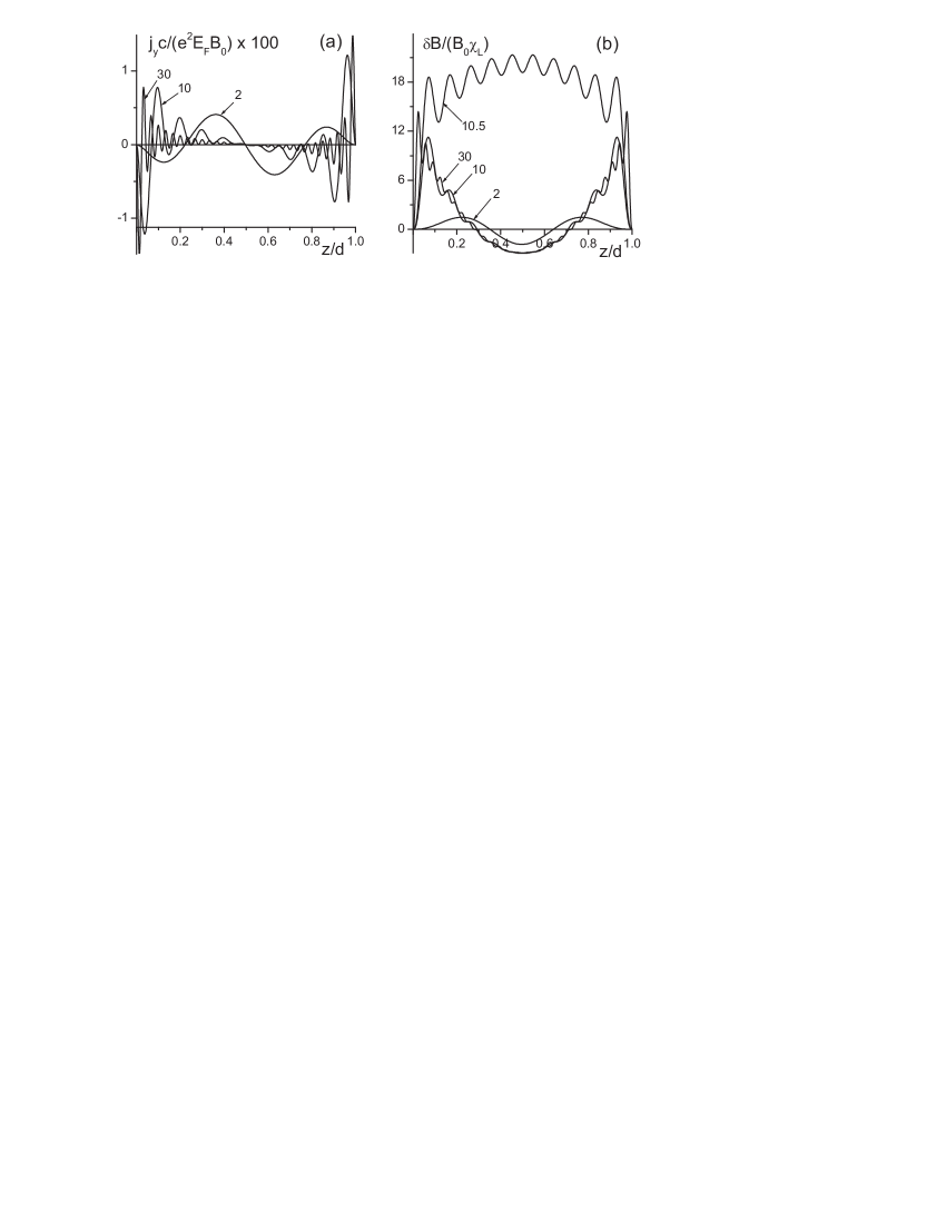
  Figure 1: Evolution of the current density (a) and magnetic field (b) for $T=0$ with the well width. The numbers of the occupied transversal subbands $k_{F}d/\pi$ are marked on curves. For $k_{F}d/\pi=2,10,30$ the Fermi energy coincides with subbands bottoms, for $k_{F}d/\pi=10.5$ it lies between 10th and 11th bottoms.

  The Fig. 1(a) depicts the current distribution in the quantum well with rectangular walls. The current density is antisymmetric in reference to the well center and oscillatory decays apart from the boundaries. The oscillations reflects the Friedel phenomenon, namely, the susceptibility singularity at the wave vector $2k_{F}$. The direction of current density alternates, so the term ”diamagnetic”, strictly speaking, refers to the integrated surface current only. In the low-temperature limit the current decay is slow. If the well width is larger than the Fermi wavelength, $2\pi/k_{F}$, the current density and magnetic field asymptotics on the small distance $z\ll d$ to the boundary read

  $$j_{y}=3\chi_{L}ck_{F}B_{0}\Bigl{(}-\frac{\cos x}{x}+3x^{2}\int\limits_{x}^{\infty}\frac{\sin t}{t^{5}}dt\Bigr{)},~{}~{}~{}\frac{\delta B}{B_{0}}=4\pi\chi_{L}\Bigl{(}1-\frac{3\sin x}{2x}+\frac{3x^{3}}{2}\int\limits_{x}^{\infty}\frac{\sin t}{t^{5}}dt\Bigr{)}$$ (5)

  Here $\chi_{L}=-e^{2}k_{F}/12\pi^{2}mc^{2}$ is the Landau diamagnetic susceptibility at $T=0$,  $x=2k_{F}z$. The first terms in Eq.(5) represent the asymptotics in the domain $z\gg\pi/k_{F}$. In particular, the constant contribution in $\delta B/B_{0}$ gives exactly the Landau magnetic permeability of a bulk sample.

  At finite temperature one can find for $k_{F}z\gg 1$

  $$\frac{\delta B}{B_{0}}=4\pi\chi_{L}\left[1-\frac{3\pi T}{4E_{F}}\frac{\sin(2k_{F}z)}{\sinh(z/l_{T})}\right],$$ (6)

  where the characteristic damping length $l_{T}=k_{F}/(2\pi mT)$. Note, that the impurity scattering also leads to the drop of $\delta B(z)$ on a distance of mean free path from the surface.

  Besides the oscillating surface diamagnetic current, Fig. 1(a) unexpectedly shows a small regular component of the current density, which is linear with the transversal coordinate. Asymptotically at $k_{F}d/\pi\gg 1$ this contribution reads as

  $$-\frac{e^{2}B_{0}k_{F}}{12mcd^{2}}(z-d/2)(1+6\zeta(\zeta-1)),~{}~{}~{}~{}~{}~{}~{}\zeta=k_{F}d/\pi-[k_{F}d/\pi].$$ (7)

  The linear component is smaller than the surface current by the factor $1/(k_{F}d)$. The sign of the slope of the linear term alternates with the chemical potential. The linear term, averaged with respect to the chemical potential (ensemble averaging) vanishes. At the finite temperature the linear term is

  $$-\frac{e^{2}TB_{0}}{\pi cd}(z-d/2)\sum\limits_{n=1}^{\infty}\frac{\cos(2nk_{F}d)}{n\sinh(nT/\theta)},$$ (8)

  where $\theta=E_{F}(\pi k_{F}d)^{-1}$ is the characteristic temperature above which the linear term washes out.

  The magnetic field corrections are shown on the Fig. 1(b). The linear term in $j_{y}$ produces the parabolic contribution to magnetic field, which is sensitive to the parameter $\zeta$. The linear term in the current density and the parabolic contribution to the magnetic field are connected with the orbital magnetism. In a quantum film the orbital contribution to the magnetic susceptibility fluctuatively grows with the width like $k_{F}d$, that corresponds to the growth of the parabolic contribution to the magnetic field.

  Paramagnetic current

  In addition to the diamagnetic current, there is also a paramagnetic current, caused by electron spins. This contribution can be found from Eq.(1) with taking into account Pauli part of the Hamiltonian $-g\mu_{B}B_{0}\sigma_{x}/2$ and spin-related component of the current density operator $\hat{\bf j}^{(sp)}=cg\mu_{B}~{}\nabla\times(\mbox{\boldmath{$\sigma$}}\delta(z-\hat{z}))/S$. Here $g$ is g-factor, $\mu_{B}$ is the Bohr magneton, $\sigma_{i}$ are Pauli matrices. As a result we find for the density of paramagnetic current

  $$j_{y}^{(sp)}=\frac{g^{2}\mu_{B}^{2}cB_{0}}{2S}\sum_{n,{\bf p}}\Bigl{(}-\frac{\partial f(E_{n{\bf p}})}{\partial E}\Bigr{)}\frac{\partial\varphi_{n}^{2}(z)}{\partial z}\equiv\frac{g^{2}\mu_{B}^{2}cB_{0}}{4}\frac{\partial}{\partial\mu}\frac{\partial}{\partial z}n(z),$$ (9)

  where $n(z)$ is the local electron concentration. This current and corresponding magnetic field should be added to the diamagnetic contributions. The ratio of diamagnetic and paramagnetic contributions depends on g-factor and, in principle, may strongly vary in different materials.

  In the specific case of square quantum well and $T=0$ we find

  $$j_{y}^{(sp)}=-\frac{g^{2}\mu_{B}^{2}mk_{F}^{2}cB_{0}}{2\pi^{2}}(\frac{\cos x}{x}-\frac{\sin x}{x^{2}}),~{}~{}~{}~{}\delta B=\frac{g^{2}\mu_{B}^{2}mk_{F}B_{0}}{\pi}(1-\frac{\sin x}{x}).$$ (10)

  Let us consider the imaginary experiment of excitation of nuclear spin transition by the alternating gate voltage. Let 2D gated system is subjected to a magnetic field with z and x components. The normal component of field stays unscreened in an infinite 2D system. The x-component of magnetic field depends on the number of electrons and their state and hence can be controlled by acting on electron subsystem. In particular, the alternating voltage, applied to the gate will modulate the magnetic field and excite the NMR transitions. The excitation of NMR transitions is possible if the alternating component of magnetic field is orthogonal to the constant magnetic field. The resonance should be detected by the frequency (or magnetic field) dependence of the gate impedance. The magnetic field is non-uniform and hence different nuclei experience different in value magnetic fields. On the one hand, this leads to inhomogeneous signal broadening, on the other hand, provides the way of separate excitation of nuclei at different depths.

  The work was supported by the Russian Fund for Basic Researches (grants 00-02-17658 and 02-02-16377).

References

- [1] M. Ya. Azbel, Aharonov-Bohm-induced Meissner-type effect and orbital ferromagnetism in normal metals. Phys.Rev. B 48, 4592(1993).
- [2] K. Richter, D. Ullmo, R. A. Jalabert, Orbital magnetism in the ballistic regime: geometrical effect. Phys. Reports 276, 1(1996).
- [3] E. Gurevich and B. Shapiro, Orbital Magnetism in Two-Dimensional Integrable Systems. J.Phys. I France 7, 807(1997).