Statistical mechanics of dissipative systems

Abstract

We propose a generalization of classical statistical mechanics which describes the behavior of dissipative systems placed in contact with a heat bath. In contrast to conventional statistical mechanics, which assigns probabilities to the states of the system, the generalized theory assigns probabilities to the trajectories of the system. The conditional probability of pairs of states at two different times is given by a path integral. We present two simple analytically-tractable examples which illustrate the predicted effect of temperature on the mean trajectories, hysteresis and drift of the system.

The fundamental question addressed in the present communication is: How does a dissipative system behave when it is placed in contact with a heat bath? It should be carefully noted that the systems under consideration are dissipative ab initio, e. g., as a result of internal friction, viscosity, or some other dissipative mechanism. In particular, the systems are irreversible, path dependent, and exhibit hysteresis. Therefore, the objective of the theory is not to understand how dissipation arises from the coarse-graining of a conservative system or in connection with first-order phase transitions (see Jiles and Atherton (1984); Ortin (1991); Sethna et al. (1993); Kinderlehrer and Ma (1997) for notable examples of that line of inquiry). Instead, the focus is in understanding how a heat bath influences the behavior of a dissipative system; what are the statistical properties of its trajectories; and how the effective behavior depends on temperature.

For definiteness, we consider systems whose state is defined by an $N$-dimensional array ${\bm{q}}$ of generalized coordinates. The energetics of the system is described by an energy function $E({\bm{q}},t)$. The explicit time dependence of $E$ may arise, e. g., as a result of the application to the system of a time-dependent external field. In addition, the system is assumed to possess viscosity, and, thus, the equilibrium equations are of the form:

$${\bm{f}}\equiv\frac{\partial E}{\partial{\bm{q}}}({\bm{q}},t)+{\bm{f}}^{\rm vis}(\dot{\bm{q}})=0$$ (1)

where ${\bm{f}}^{\rm vis}$ are the viscous forces. These equilibrium equations define a set of ordinary differential equations which, given appropriate conditions at, e. g., $t=0$, can be solved for the trajectory ${\bm{q}}(t)$, $t\geq 0$.

If the system is conservative, i. e., if ${\bm{f}}^{\rm vis}={\bf 0}$, the instantaneous state ${\bm{q}}(t)$ of the system at time $t$ follows directly from energy minimization, i. e., from the problem:

$$E\big{(}{\bm{q}}(t),t\big{)}=\min_{{\bm{q}}^{\prime}\in{\mathbb{R}^{N}}}E({\bm{q}}^{\prime},t)$$ (2)

In order to extend this variatonal framework to dissipative systems, we resort to time discretization, leading to a sequence of minimization problems of the form (2) Ortiz and Repetto (1999); Radovitzky and Ortiz (1999); Ortiz and Stainier (1999). Thus, we consider a time-discretized incremental process consisting of a sequence of states ${\bf q}_{n-1}$ at times $t_{0}=0$, $\dots$, $t_{n-1}$, $t_{n}=t_{n-1}+{\triangle t}$, $\dots$. We additionally assume that the viscous forces ${\bm{f}}^{\rm vis}$ derive from a kinetic potential $\phi(\dot{\bm{q}})$ through the relation:

$${\bm{f}}^{\rm vis}=\frac{\partial\phi}{\partial\dot{\bf q}}(\dot{\bm{q}})$$ (3)

and introduce the incremental work function:

$$\begin{split}&W({\bm{q}}_{n},{\bm{q}}_{n-1})=E({\bm{q}}_{n})-E({\bf q}_{n-1})\\ &+\min_{\{paths\}}\int^{t_{n}}_{t_{n-1}}\phi\big{(}\dot{\bf q}(t)\big{)}\,dt\end{split}$$ (4)

where the minimum is taken over all paths ${\bm{q}}(t)$ such that ${\bm{q}}(t_{n-1})={\bm{q}}_{n-1}$ and ${\bm{q}}(t_{n})={\bm{q}}_{n}$. The fundamental property of the incremental work function $W({\bf q}_{n},{\bm{q}}_{n-1})$ is that it acts as a potential for the forces ${\bm{f}}_{n}$ at time $t_{n}$, i. e.,

$${\bm{f}}_{n}=\frac{\partial W}{\partial{\bm{q}}_{n}}({\bm{q}}_{n},{\bf q}_{n-1})$$ (5)

In order to verify this property, we may consider a small perturbation ${\bm{q}}_{n}\to{\bm{q}}_{n}+\delta{\bm{q}}_{n}$, leading to a corresponding perturbation of the path ${\bm{q}}(t)\to{\bm{q}}(t)+\delta{\bm{q}}(t)$, with $\delta{\bm{q}}(t_{n-1})=\delta{\bm{q}}_{n-1}={\bf 0}$. Then, in follows that

$$\begin{split}&\delta W({\bm{q}}_{n},{\bm{q}}_{n-1})=\frac{\partial E}{\partial{\bm{q}}}({\bm{q}}_{n})\cdot\delta{\bm{q}}_{n}+{\bm{f}}^{\rm vis}_{n}\cdot\delta{\bm{q}}_{n}\\ &+\int^{t_{n}}_{t_{n-1}}{\bm{f}}^{\rm vis}\big{(}\dot{\bm{q}}(t)\big{)}\cdot\delta\dot{\bm{q}}(t)\,dt\end{split}$$ (6)

But the integral on the right hand side of this equation is to be evaluated along the minimizing path, and hence it vanishes identically. This gives the identity

$$\delta W({\bm{q}}_{n},{\bm{q}}_{n-1})=\left\{\frac{\partial E}{\partial{\bm{q}}}({\bm{q}}_{n})+{\bm{f}}^{\rm vis}_{n}\right\}\cdot\delta{\bf q}_{n}$$ (7)

Since the variation $\delta{\bm{q}}_{n}$ is arbitrary, it follows that

$$\frac{\partial W}{\partial{\bm{q}}_{n}}({\bm{q}}_{n},{\bm{q}}_{n-1})=\frac{\partial E}{\partial{\bm{q}}}({\bm{q}}_{n})+{\bm{f}}^{\rm vis}_{n}={\bm{f}}_{n}$$ (8)

as stated. From this property it follows that the equilibrium equation ${\bm{f}}_{n}={\bf 0}$ is the Euler-Lagrange equation corresponding to the minimum principle:

$$\min_{{\bm{q}}_{n}}W({\bm{q}}_{n},{\bm{q}}_{n-1})$$ (9)

This behavior is indistinguishable from that a conservative system with ‘energy’ $W({\bm{q}}_{n},{\bm{q}}_{n-1})$. However, it should be carefully noted that $W$ is determined by both the energetics and the kinetics of the system. Consequently, $W$ depends on the initial conditions ${\bm{q}}_{n-1}$ for the time step and, therefore, varies from step to step, which in turn allows for path dependency and hysteresis, as required. A simple situation arises when the kinetic potential $\phi(\dot{{\bm{q}}})$ is convex and coercive, i. e., it grows as $|\dot{{\bm{q}}}|^{p}$, for some $p\in(1,\infty)$, for large $|\dot{{\bm{q}}}|$. Then, the minimizing path is unique and consists of a straight segment joining ${\bm{q}}_{n-1}$ and ${\bm{q}}_{n}$. Under these conditions, the corresponding incremental work function is

$$W({\bm{q}}_{n},{\bm{q}}_{n-1})=E({\bm{q}}_{n})-E({\bm{q}}_{n-1})+\triangle t\,\phi\left(\frac{\triangle{\bm{q}}}{\triangle t}\right)$$ (10)

where we write $\triangle{\bm{q}}={\bm{q}}_{n}-{\bm{q}}_{n-1}$.

Now, imagine placing the system just described in contact with a heat bath at absolute temperature $T$. The objective is to predict the ensuing behavior of the system. For conservative systems, such behavior is predicted by standard Gibbsian statistical mechanics, to wit: the probability of finding a state ${\bm{q}}$ at time $t$ obeys Boltzmann’s distribution, i. e., is proportional to $\exp\{-\beta E({\bm{q}},t)\}$, where $\beta=1/k_{B}T$ and $k_{B}$ is Boltzmann’s constant. In particular, the states of the system at two different times are uncorrelated. We proceed to show that the analogy between the minimum principles (2) and (9) provides a basis for generalizing Gibbs’s prescription to dissipative systems. However, in contrast to conventional statistical mechanics, which assigns probabilities to the states of the system, the extended theory assigns probabilities to the trajectories of the system.

We begin by assuming that the incremental processes are Markovian, i. e., ${\bm{q}}_{n}$ is correlated to ${\bm{q}}_{n-1}$ but not to earlier states. Let $p({\bm{q}}_{n},{\bm{q}}_{n-1})$ be the joint probability of ${\bm{q}}_{n}$ and ${\bm{q}}_{n-1}$, and let

$$p({\bm{q}}_{n-1})=\int p({\bm{q}}_{n},{\bm{q}}_{n-1})\,d^{N}q_{n}$$ (11a)

$$p({\bm{q}}_{n})=\int p({\bm{q}}_{n},{\bm{q}}_{n-1})\,d^{N}q_{n-1}$$ (11b)

be the corresponding probabilities of ${\bm{q}}_{n}$ and ${\bf q}_{n-1}$. Then the conditional probability of ${\bm{q}}_{n}$ given ${\bm{q}}_{n-1}$ is

$$p({\bm{q}}_{n}|{\bm{q}}_{n-1})=\frac{p({\bm{q}}_{n},{\bm{q}}_{n-1})}{p({\bf q}_{n-1})}$$ (12)

This probability may also be interpreted as the transition probability from state ${\bm{q}}_{n-1}$ to the new state ${\bf q}_{n}$. We postulate that the transition probability $p({\bm{q}}_{n}|{\bm{q}}_{n-1})$ is Gibbsian, i. e.,

$$p({\bm{q}}_{n}|{\bm{q}}_{n-1})=\frac{1}{Z({\bm{q}}_{n-1})}e^{-\beta W({\bf q}_{n},{\bm{q}}_{n-1})}$$ (13)

where

$$Z({\bm{q}}_{n-1})=\int e^{-\beta W({\bm{q}}_{n},{\bm{q}}_{n-1})}\,d^{N}q_{n}$$ (14)

is an incremental partition function. It therefore follows that:

$$p({\bm{q}}_{n})=\int\frac{1}{Z({\bm{q}}_{n-1})}e^{-\beta W({\bf q}_{n},{\bm{q}}_{n-1})}p({\bm{q}}_{n-1})\,d^{N}q_{n-1}$$ (15)

Iterating this relation we obtain

$$\begin{split}&p({\bm{q}}_{n})=\\ &\int\dots\int\left\{\prod_{i=0}^{n-1}\frac{e^{-\beta W({\bm{q}}_{i+1},{\bm{q}}_{i})}}{Z({\bm{q}}_{i})}\right\}\,p({\bm{q}}_{0})\,d^{N}q_{n-1}\dots d^{N}q_{0}\end{split}$$ (16)

In the limit of ${\triangle t}\to 0$ and $n\to\infty$ at fixed $t=n{\triangle t}$, (16) defines a path integral of the form (see, e. g., Wiegel (1986)):

$$p({\bm{q}}_{t}|{\bm{q}}_{0})=\int\dots\int e^{-\beta\mathcal{W}[{\bm{q}}]}\mathcal{D}q$$ (17)

for some system-dependent work functional $\mathcal{W}[{\bm{q}}]$. This path integral gives the conditional probability $p({\bm{q}}_{t}|{\bm{q}}_{0})$ of finding the system in state ${\bm{q}}_{t}$ at time $t\geq 0$ given that the system is in state ${\bm{q}}_{0}$ at time $t=0$. The integrand of (17) may be interpreted as relating to the probability of individual trajectories $q(\tau)$. More precisely, given two trajectories ${\bm{q}}_{1}(\tau)$ and ${\bm{q}}_{2}(\tau)$, their relative probabilities are:

$$\frac{p[{\bm{q}}_{1}]}{p[{\bm{q}}_{2}]}=\frac{e^{-\beta W[{\bm{q}}_{1}]}}{e^{-\beta W[{\bm{q}}_{2}]}}$$ (18)

It is noteworthy that, in contrast to the conservative case, the presence of kinetics renders states of the system at different types correlated. However, this correlation may be expected to decay with elapsed time, conferring the system a fading memory property.

In the remainder of this letter we present two simple analytically-tractable examples which provide a first illustration of the theory, namely: a linear spring-dashpot system; and dry friction. In addition to their value as illustrative examples, these simple models should also useful as a basis for constructing mean-field approximations to more complex systems. The treatment of general systems requires the use of numerical schemes such as the Path-Integral Monte Carlo (PIMC) method Binder (1992).

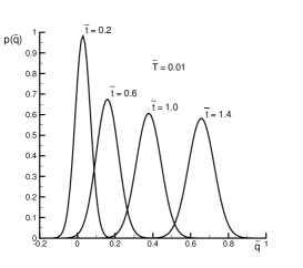
Figure 1: Evolution of the probability density for a spring and dashpot system subjected to time-proportional loading.

The linear spring-dashpot system is characterized by an energy function and kinetic potential of the form:

$$E(q,t)=\frac{\kappa}{2}q^{2}-f(t)q$$ (19a)

$$\phi(\dot{q})=\frac{\eta}{2}\dot{q}^{2}$$ (19b)

where $q\in\mathbb{R}$, $\kappa$ is the spring constant, $\eta$ is the dashpot viscosity, and $f(t)$ is a time-dependent applied force. For this system, the equilibrium equations (1) reduce to:

$$\kappa q-f+\eta\dot{q}=0$$ (20)

The corresponding incremental work function for this system is:

$$\begin{split}&W(q_{n},q_{n-1})=\frac{\kappa}{2}(q_{n}^{2}-q_{n-1}^{2})\\ &-f_{n}q_{n}+f_{n-1}q_{n-1}+\frac{\eta}{2{\triangle t}}(q_{n}-q_{n-1})^{2}\end{split}$$ (21)

and the evaluation of the partition function entails a simple Gaussian integral. Inserting the result in (16) yields

$$\begin{split}&p(q_{n})=\int\dots\int\left(\frac{2\pi}{\beta(\kappa+\eta/{\triangle t})}\right)^{-n/2}\\ &\exp\left\{-\beta\sum_{i=0}^{n-1}\frac{\big{(}{\triangle t}(f_{i+1}-\kappa q_{i+1})-\eta(q_{i+1}-q_{i})\big{)}^{2}}{2{\triangle t}(\eta+\kappa{\triangle t})}\right\}\\ &p(q_{0})\,dq_{n-1}\dots dq_{0}\end{split}$$ (22)

In the limit of ${\triangle t}\to 0$ and $n\to\infty$, with $t=n{\triangle t}$ fixed, the sum in the exponential of this formula converges to the Riemann integral

$$\mathcal{W}[q]=\int_{0}^{t}\frac{1}{2\eta}\big{(}\kappa q(\tau)-f(\tau)+\eta\dot{q}(\tau)\big{)}^{2}\,dt$$ (23)

In the same limit, (22) may be written as the path integral

$$\mathcal{D}q=\lim_{n\to\infty}\left(\frac{2\pi}{\beta\big{(}\kappa+\eta/(t/n)\big{)}}\right)^{-n/2}\,dq_{n-1}\dots dq_{0}$$ (24)

which is of the anticipated form (17). The structure of (17) is revealing. Thus, it is observed that the work functional $\mathcal{W}[q]$ integrates in time the square of the equilibrium equation (20), reduced to units of power by means of the factor $1/\eta$. Evidently, the path which contributes the most to the path integral is the critical path, i. e., the path $q_{c}$ which minimizes the work functional (23). Indeed, in the limit of zero viscosity or zero temperature, the only path which contributes to the path integral is the critical path, which in that limit coincides with the deterministic trajectory, i. e., with the solution of (20). For finite viscosity and finite temperature, however, all paths contribute to the path integral to varying degrees, the contributions becoming increasingly weaker as the trajectories depart from the critical path. The stationarity of $\mathcal{W}[q]$ yields the Euler-Lagrange equations for the critical path

$$\ddot{q}-\omega^{2}q=\frac{\dot{f}}{\eta}-\omega^{2}\frac{f}{\kappa}$$ (25)

where $\omega=\kappa/\eta$ and the solution $q_{c}$ is subject to the boundary conditions $q_{c}(0)=q_{0}$, $q_{c}(t)=q_{t}$. It is interesting to note that this equation is of second order in time, whereas the original equilibrium equation (20) is of first order. This increase in order makes it possible to enforce boundary conditions at times $0$ and $t$, in contrast to the original equation (20) which only allows for initial conditions. Furthermore, we note that (25) is obtained by squaring (20), and thus the solutions of the latter are subsumed within the former. However, by virtue of its higher order the Euler-Lagrange equation (25) has solutions which do not satisfy (20). It thus follows that the critical path does not coincide with the deterministic trajectory in general. Conveniently, the path integral (17) can be evaluated exactly in closed form (e. g., Wiegel (1986) and Feynman (1990)). The result is:

$$p(q_{t})=\sqrt{\frac{\beta\kappa e^{\omega t}}{2\pi\sinh(\omega t)}}e^{-\beta(\mathcal{W}[q_{c}])}$$ (26)

where the critical path $q_{c}(t)$ is the solution of (25). Fig. 1 shows the evolution of the probability density for a linear loading history $f(t)=At$ in terms of the normalized variables $\tilde{q}=q/(A\eta/\kappa^{2})$, $\tilde{t}=t/(\eta/\kappa)$, and $\tilde{T}=T/(A^{2}\eta^{2}/k_{B}\kappa^{3})$. The mean value $\langle q(t)\rangle$ traces the critical path $q_{c}(t)$, which, as noted earlier, differs from the classical path at finite viscosity and temperature. An additional effect of viscosity, which is clearly evident in these figures, is to cause the width of the probability density to broaden in time, with the attendant increase in the uncertainty of the state of the system.

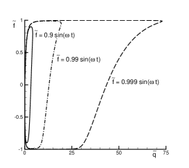
Figure 2: Trajectories of a system sliding under the action of an applied cyclic load $f(t)=A\,\sin(\omega t)$ against a frictional resistance $s$.

The work functional (23) appearing in the path integral representation (17) is characteristic of systems whose kinetic potential $\phi(\dot{{\bm{q}}})$ exhibits quadratic behavior near the origin. However, there are cases of interest which do not fall into that category. A case in point is provided by dry friction, which is characterized by a kinetic potential which has a vertex at the origin. Consider, by way of example, a one-dimensional system sliding against a frictional resistance $s>0$ under the action of an applied force $f(t)$ such that $|f(t)|\leq s$. In this particular case

$$E(q,t)=-f(t)q$$ (27a)

$$\phi(\dot{q})=s|\dot{q}|$$ (27b)

and the incremental work function (4) specializes to

$$W(q_{n},q_{n-1})=-f_{n}q_{n}+f_{n-1}q_{n-1}+s\,|q_{n}-q_{n-1}|$$ (28)

As expected from the rate-independent nature of dry friction, $W$ is independent of $\triangle t$. The corresponding partition function (14), transition probability (13), and probability density (16) take the form:

$$Z(q_{n-1})=\frac{2s}{\beta(s^{2}-f_{n}^{2})}{\rm e}^{\beta(f_{n}-f_{n-1})\,q_{n-1}}$$ (29)

$$p(q_{n}|q_{n-1})=\frac{\beta(s^{2}-f_{n-1}^{2})}{2s}{\rm e}^{s\,|q_{n}-q_{n-1}|-f_{n}(q_{n}-q_{n-1})}$$ (30)

and

$$\begin{split}&p(q_{n})=\int\dots\int\prod_{i=0}^{n-1}\frac{\beta(s^{2}-f_{i}^{2})}{2s}\\ &\exp\left\{-\beta\sum_{i=0}^{n-1}\big{(}s\,|q_{i+1}-q_{i}|-f_{i+1}(q_{i+1}-q_{i})\big{)}\right\}\\ &p(q_{0})\,dq_{n-1}\dots dq_{0}\end{split}$$ (31)

respectively. An important feature of the transition probability (30) is that it depends solely on the difference $q_{n}-q_{n-1}$. Therefore, the chain $q_{0}$, $q_{1}$, $\dots$, $q_{n}$ defines a random walk, and the probability $p(q_{t}|q_{0})$ corresponding to the limit of ${\triangle t}\to 0$ and $n\to\infty$ at constant $t=n{\triangle t}$ follows by an application of the central limit theorem. The result is:

$$p(q_{t}|q_{0})=\frac{1}{\sqrt{2\pi}\sigma(t)}{\rm e}^{-\big{(}q_{t}-\langle q\rangle(t)\big{)}^{2}/2\sigma^{2}(t)}$$ (32)

where

$$\begin{split}\langle q\rangle(t)&=q_{0}+\lim_{n\to\infty}\frac{1}{n}\sum_{i=0}^{n-1}\frac{2f_{i}}{\beta(s^{2}-f_{i}^{2})}\\ &=q_{0}+\frac{1}{t}\int_{0}^{t}\frac{2f(\tau)}{\beta\big{(}s^{2}-f^{2}(\tau)\big{)}}\,d\tau\end{split}$$ (33)

is the mean path traced by the system, and

$$\begin{split}\sigma^{2}(t)&=\lim_{n\to\infty}\frac{1}{n}\sum_{i=0}^{n-1}\frac{2(s^{2}+f_{i}^{2})}{\beta^{2}(s-f_{i})^{2}(s+f_{i})^{2}}\\ &=\frac{1}{t}\int_{0}^{t}\frac{2\big{(}s^{2}+f^{2}(\tau)\big{)}}{\beta^{2}\big{(}s-f(\tau)\big{)}^{2}\big{(}s+f(\tau)\big{)}^{2}}\end{split}$$ (34)

measures the deviation from the mean path. It is interesting to note that, in the limit of zero temperature, $\langle q\rangle(t)=q_{0}$ for as long as $|f(t)|<s$, with the system sliding off to $\pm\infty$ instantaneously as soon as $f$ reaches $\pm s$. By way of sharp contrast, at finite temperature the system undergoes sliding even when the applied force $f(t)$ remains strictly below $s$ in magnitude at all times. In addition, the standard deviation $\sigma$ from the mean path is predicted to be proportional to temperature. By way of illustration of this behavior, the trajectories of the system corresponding to applied cyclic loads of the form $f(t)=A\,\sin(\omega t)$ are shown in Fig. 2 in terms of the normalized variables: $\bar{q}=q/(k_{B}T/s)$, $\bar{f}=f/s$, and $\bar{t}=\omega t$. The ability of the theory to allow for hysteresis and to predict its temperature dependence is particularly noteworthy. As expected, the response of the system is predicted to soften with increasing temperature, in keeping with numerical simulations of magnetic systems Nowak et al. (1997).

References

- Sethna et al. (1993) J. P. Sethna, K. Dahmen, S. Kartha, J. A. Krumhansl, B. W. Roberts, and J. D. Shore, Physical Review Letters 70, 3347 (1993).
- Ortin (1991) J. Ortin, Journal of Applied Physics 71, 1454 (1991).
- Kinderlehrer and Ma (1997) D. Kinderlehrer and L. Ma, Journal of Nonlinear Science 23, 101 (1997).
- Jiles and Atherton (1984) D. C. Jiles and D. L. Atherton, Journal of Applied Physics 55, 2115 (1984).
- Ortiz and Stainier (1999) M. Ortiz and L. Stainier, Computer Methods in Applied Mechanics and Engineering 171, 419 (1999).
- Ortiz and Repetto (1999) M. Ortiz and E. Repetto, Journal of the Mechanics and Physics of Solids 47, 397 (1999).
- Radovitzky and Ortiz (1999) R. Radovitzky and M. Ortiz, Computer Methods in Applied Mechanics and Engineering 172, 203 (1999).
- Wiegel (1986) F. W. Wiegel, Introduction to Path-Integral Methods in Physics and Polymer Science (World Scientific, 1986).
- Binder (1992) K. Binder, ed., The Monte Carlo Method in Condensed Matter Physics (Springer-Verlag, New York, 1992).
- Feynman (1990) R. P. Feynman, Statistical Mechanics. A set of lectures, vol. 36 of Frontiers in Physiscs (Addison Wesley, 1990), 13th ed.
- Nowak et al. (1997) U. Nowak, J. Heimel, T. Kleinefeld, and D. Weller, Physics Review B 56, 8143 (1997).