Topological correlations in trivial knots: new arguments in support of the crumpled polymer globule

Abstract

We prove the fractal crumpled structure of collapsed unknotted polymer ring. In this state the polymer chain forms a system of densely packed folds, mutually separated in all scales. The proof is based on the numerical and analytical investigation of topological correlations in randomly generated dense knots on strips $L_{v}\times L_{h}$ of widths $L_{v}=3,5$. We have analyzed the conditional probability of the fact that a part of an unknotted chain is also almost unknotted. The complexity of dense knots and quasi–knots is characterized by the power $n$ of the Jones–Kauffman polynomial invariant. It is shown, that for long strips $L_{h}\gg L_{v}$ the knot complexity $n$ is proportional to the length of the strip $L_{h}$. At the same time, the typical complexity of the quasi–knot which is a part of trivial knot behaves as $n\sim\sqrt{L_{h}}$ and hence is significantly smaller. Obtained results show that topological state of any part of the trivial knot in a collapsed phase is almost trivial.

I Introduction

It is well known, that very often new interesting problems appear at the edges of traditional fields of science. Statistical topology, emerged from statistical physics, theory of integrable systems and algebraic topology can be regarded as an example of such new joint area. The scope of problems dealing with construction of knot and link invariants as well as study of entropy of random knots belongs to this field.

In this paper the modern methods of algebraic topology are used to argue for the nontrivial fractal structure of unknotted polymer ring in a compact state. Namely, we show that the condition for the whole knot to be trivial implies that each part of such knot in the compact state is almost unknotted.

Let us remind that the non-phantomness of polymer chains causes two types of interactions: a) volume interactions, vanishing for infinitely thin chains, and b) topological interactions, remaining even for chains of zero thickness. For sufficiently high temperatures the polymer macromolecule is strongly fluctuating system without reliable thermodynamic state. However for temperatures below some critical value $\theta$ the macromolecule forms a dense drop–like weakly fluctuating globular structure lif ; lgkh . In classical works lif ; lgkh devoted to investigation of coil–to–globule phase transition without topological constraints it has been shown, that for $T<\theta$ the globular state can be described in virial approximation, i.e. using only two– and three–body interaction constants: $B=b\frac{T-\theta}{\theta}<0$ and $C={\rm const}>0$ (see also grosbk ). The approach developed in lif ; lgkh is considered as the basis of the modern statistical theory of collapsed state of polymer systems.

In the globular phase of unknotted macromolecule the topological constraints play a role of an additional repulsion. One might expect that the parts of the unknotted chain deeply penetrate each other by loops as it is shown in Fig.1a. However this is not true and in the paper gns it has been shown that the absence of knots on densely packed polymer ring causes very unusual fractal properties of the chain trajectory strongly affecting all the thermodynamic properties of the macromolecule in the globular phase. The corresponding structure of a collapsed unknotted polymer ring was named ”crumpled” fractal globule. The chain trajectory in the crumpled globule densely fills the volume such that all parts of the chain become segregated from each other in a broad region of scales—see Fig.1. Hence, the line path in a crumpled globule reminds the well known Peano curve man schematically shown in Fig.1c.

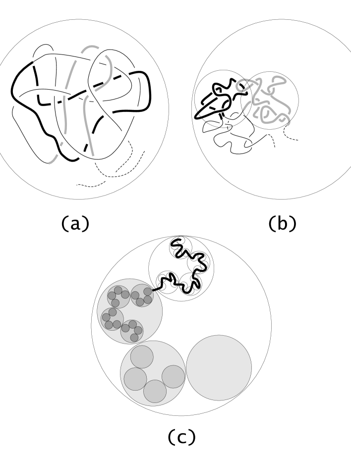
Figure 1: a) The globular (collapsed) state of a polymer chain with an arbitrary loop penetrating to the size of a whole globule; b) The crumpled globular state with a test loop segregated ”in itself”. This structure resembles the Peano curve schematically shown in c).

Experimental examination of a fractal structure of unknotted polymer ring is a very difficult problem. Some measurements can be interpreted as the indirect verification of the crumpled globule structure: a two–stage dynamics of a collapse of a linear macromolecule after abrupt change of a solvent quality chu and the effect of compatibility enhancement in a melt of linear and ring macromolecules mcknight . However now there was no direct observation of crumpled globule structure in equilibrium globular polymer chains.

We show below that the investigation of distribution of random knots over the topological classes and analysis of topological correlations in trivial knots helps one to understand the structure of the phase space of unknotted polymer in a globule phase and validate the crumpled globule conjecture ”from the first principle”.

II The model of dense knots and a concept of ”quasi–knots”

Below we express the arguments in support of the crumpled globule on the basis of direct determination of the topological state of a part of a polymer chain under the condition that the chain as a whole forms an unknotted loop. In our work we use some modern methods of construction of topological knot invariants jones ; kauffman ; wu applied for solution of specific statistical problems grne_alg ; vasne .

First of all one has to define the topological state of a part of a ring polymer chain. Certainly, the mathematically rigorous definition of the topological state exists for closed or infinite paths. Nevertheless, the everyday’s experience tells us that open but sufficiently long rope can be knotted. Hence, it is desirable to introduce the concept of a quasi–knot available for topological description of open paths.

For the first time that idea in the polymer context had been formulated by I.M. Lifshits and A.Yu. Grosberg ligr . They argued that the topological state of a linear polymer chain in a globular state is defined much better than topological state of a coil. Actually, the distance between the ends of the chain in a globule is of order $R\sim aN^{1/3}$, where $a$ is a size of a monomer and $N$ is a number of monomers in a chain. Taking into account that $R$ is sufficiently smaller than the contour length $N$ and that the density fluctuations are negligible, we may define the topological state of a path in a globule as a topological state of composition of a chain itself and a segment connecting its ends. This composite structure can be regarded as a quasi–knot for an open chain in a globular state. Later on we shall repeatedly use this definition.

Let us describe the model under consideration. The crumpled globule is modeled by ”dense” knots. We call the knot ”dense” if its projection onto the plane fully fills the rectangle lattice $M$ of size $L_{v}\times L_{h}$ — see Fig.2.

Figure 2: The trivial knot $3\times 5$ and the knot $3\times 3$ obtained by cutting a knot $3\times 5$.

The lattice $M$ is filled densely by a single thread, which crosses itself in each vertex of the lattice in two different ways: ”above” or ”below”. The topology of a knot is defined by ”above” and ”below” passages with prescribed boundary conditions. The ”woven carpet” shown in Fig.2 corresponds to a trivial knot. Let use enumerate the vertices of the lattice by the index $k$ and attribute to each vertex the variable $\epsilon_{k}$ according to the rule:

Our task can be rephrased now as follows. We have an ensemble of randomly generated crossings $\{\epsilon_{k}\}$

$$\left\{\begin{array}[]{ll}\epsilon_{k}=-1&\mbox{with probability $p$}\\ \epsilon_{k}=+1&\mbox{with probability $1-p$}\end{array}\right.$$

independent in all vertices under the condition that the total set of crossings $\{\epsilon_{k}\}$ defines a trivial knot. We call this initial knot the ”parent” one. If $\epsilon_{k}=+1$ for all $k=[1,N]$ then the knot is trivial. Changing the sign for some $\epsilon_{k}$ from ”$+$” to ”$-$” we can get a nontrivial knot. Later we shall call such change of a sign ”impurity”, so $p$ is concentration of impurities. Let us cut a part of the parent trivial knot closing the open ends of the threads as it is shown in Fig.2. This way we get the well–defined ”daughter” quasi–knot. Below we study the typical topological state of such daughter quasi–knots under the condition that the parent knot is trivial.

The model under consideration is oversimplified because it does not take into account the spatial fluctuations of a path of a polymer chain in a knot. However we believe that our model well describes the globular (condensed) structure of a polymer ring where the chain fluctuations are essentially suppressed and the polymer has reliable thermodynamic structure with almost constant density ligr .

III Topological invariants and knot complexity

In our work we characterize the topological state of the knot by its Jones–Kauffman polynomial invariant jones ; kauffman . Recall that the Kauffman invariant of variable $A$ is a Jones polynomial of variable $x=A^{4}$ kauffman .

In brief the procedure of construction of the algebraic knot invariant is as follows. Let us construct the ”Potts lattice” $\Lambda$ corresponding to the ”knot lattice” $M$—see Fig.3b.

Figure 3: a) The trivial knot $3\times 5$; b) The lattice of Potts spins, corresponding to the trivial knot $3\times 5$; c) The lattice of Potts spins transformed to $2\times 6$—strip corresponding to the trivial knot $3\times 5$; d) The transfer matrix, corresponding to ferro– and antiferro–magnetic bonds on the Potts lattice.

In Fig.3a positions of Potts spins are depicted by circles. Introduce the set of variables $b_{i,j}$ on the bonds of the Potts lattice as follows:

$$b_{i,j}=\left\{\begin{array}[]{cl}-\epsilon_{k},&\mbox{for right--down bond ($i,j$)}\\ \epsilon_{k},&\mbox{for right--up bond ($i,j$)}\end{array}\right.$$ (1)

We can treat $b_{i,j}=1$ and $b_{i,j}=-1$ as ”ferromagnetic” and ”antiferromagnetic” bonds, because changing a sign $b_{i,j}$ means changing a sign of the coupling constant $J_{i,j}$. Let us note, that even for the trivial knot we have antiferromagnetic bonds on the Potts lattice — see Fig.3a and Fig.3b,c. We should stress that in our terms the ”impurity” means not an antiferromagnetic bond, but just the change of the sign of a bond with respect to the trivial knot. In Fig.3b and Fig.3c the ferromagnetic $b_{i,j}=1$ and antiferromagnetic $b_{i,j}=-1$ bonds are shown by solid and dashed lines correspondingly.

In grne_alg ; vasne it has been explicitly shown that the Jones knot invariant $f_{K}(x)$ of variable $x$ of ambiently isotopic knots on the lattice $M$ can be expressed as a partition function of the Potts model on the lattice $\Lambda$:

$$f_{K}(x,\{b_{i,j}\})=K\left(x,\{b_{i,j}\}\right)Z\Big{(}q(x),\{J_{i,j}(b_{i,j},x)\}\Big{)}$$ (2)

where

$$K\left(x,\{b_{i,j}\}\right)=\left(-\sqrt{x}-\frac{1}{\sqrt{x}}\right)^{-(N_{p}+1)}\left(-\sqrt{x}\right)^{\sum\limits_{\{i,j\}}b_{i,j}}$$ (3)

is a trivial prefactor, independent on Potts spins and $N_{p}=\frac{1}{2}(L_{v}+1)(L_{h}+1)$ is a total number of Potts spins.

The Potts partition function $Z\Big{(}q(x),\{J_{i,j}(b_{i,j},x)\}\Big{)}$ defined in (2) reads:

$$Z\Big{(}q(x),\{J_{i,j}(b_{i,j},x)\}\Big{)}=\sum\limits_{\{\sigma\}}\exp\left(\sum\limits_{\{i,j\}}\frac{J_{i,j}(b_{i,j},x)}{T}\delta(\sigma_{i},\sigma_{j})\right)$$ (4)

where the coupling constant $J_{i,j}$ and the number of spin states $q$ are:

$$\frac{J_{i,j}}{T}=\ln(-x^{b_{i,j}}),\quad q=x+2+x^{-1}$$ (5)

The specific property of the partition function (4) consists in the relation between the temperature $T$ and the number of the Potts spins states, $q$, so the variables $T$ and $q$ cannot be considered as independent quantities. Later on we shall be interested in the largest power of the Jones polynomial invariant, hence we forget about specific physical sense of the parameters $x$, $T$, and $J_{i,j}$.

In the paper vasne we have investigated semi–numerically the probability $P\{f_{K}\}$ that among $2^{N}$ possible realizations of the disorder $\{\epsilon_{k}\},\;k=1,\dots,N$ one can find a knot in a specific topological state defined by the Jones–Kauffman invariant $f_{K}$.

$$P_{N}\{f_{K}\}=\frac{1}{2^{N}}\sum\limits_{\{\epsilon_{k}\}}\Delta\Big{(}f_{K}(x,\{\epsilon_{1},\dots,\epsilon_{N}\})-f_{K}\Big{)}$$

The topological disorder described by random variables $\epsilon_{k}=\pm 1$ can be considered as a quenched random disorder in an appropriate Potts model. Each topological type of a knot is characterized by polynomial invariant $f_{K}(x)$. However it is sufficient and more convenient for our particular goals to discriminate knots by more rough characteristics – the power $n$ of the polynome $f_{K}(x)$:

$$n=\lim_{|x|\to\infty}\frac{\ln f_{K}(x)}{\ln x}$$ (6)

For trivial knots $n=0$; as the knot becomes more complex, $n$ grows up to its maximal value $n\sim N$.

Certainly, the lack of our description consists in the fact that $n$ is rather rough characteristic and one cannot distinguish ”topologically similar” knots. However the discrimination of the topological state of knots (or links) by the power $n$ of a corresponding polynome enables us to introduce a ”metric” in the phase space of topological states and, hence, to compare the knots.

IV Topological correlations of (quasi)knots on the strip

In this section by numerical and analytical methods we investigate the typical topological state of a part of a ”parent” knot under the condition that the parent knot is trivial. In fact, we slightly modify the very problem as soon as we characterize the topological state of the knot by the power $n$ of its algebraic polynome. Namely, we study topological correlations not only in trivial knots, but in all knots characterized by zero’s power of the knot polynome as well. There are some non-trivial knots among a variety of knots with $n=0$, but the complexity of such non-trivial knots is not high. We could say that the knots with $n=0$ are ”about trivial”.

In our numerical investigation we restrict ourselves to topological correlations in knots represented by strips of sizes $L_{v}\times L_{h}$, where $L_{v}$ is the width ($L_{v}=3,\,5$) and $L_{h}$ is the length of the strip. We consider essentially asymmetric distribution of crossings, namely with $p=0.05,0.1$. Remind that $p=0$ corresponds to the single configuration of crossings representing the trivial knot.

IV.1 Unconditional distribution

IV.1.1 The mean complexity of the knots

The power of the polynomial invariant characterizes the complexity of a knot. Hence, according to (6) and definition of Kauffman invariant as Potts partition function, the power $n$ has a sense of a free energy. Thus, for long strips ($L_{h}\gg L_{v}$) neglecting the boundary effects produced by shorter side $L_{v}$ we conclude that $n$ is proportional to $L_{h}$. This fact directly follows from the additivity of the free energy. At the same time for short strips $L_{h}\sim L_{v}$ the boundary effects cause the deviation from linear behavior of $n$ upon $L_{h}$.

Our numerical computations remarkable confirm the above statement. The mean complexity $n(L_{h};p)$ of knots on the strip of width $L_{v}=3$ and results of the approximation (Table 1) are shown in Fig.4a.

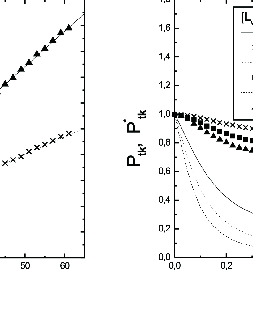
Figure 4: a) Mean largest power $n(L_{h};p)$ of polynomial invariant of a knot on a strip of width $L_{v}=5$ and length $L_{h}$ for concentrations of impurities $p=0.05,0.1$; b) Probability of a trivial knot $P_{tk}(L_{h};p)$ on the lattice $3\times L_{h}$ for $L_{h}=3,5,7$ (lines) and conditional probability of trivial daughter (quasi)knot $P^{*}_{tk}(L_{h};p)$ on a strip of width $L_{v}=3$ and length $L_{h}$ as function of $p$ under condition that the parent knot $L_{t}=2L_{h}+1$ is trivial (crosses, squares, triangles).

The corresponding data for the strip of the widths $L_{v}=3$ and $L_{v}=5$ are shown in Table 1. We have averaged the results over $30\,000$ realizations of topological disorder for each $L_{h}$. To estimate the numerical error we have splitted the ensemble of realizations onto 10 subsets of 3000 configurations each.

Table 1

$L_{v}=3$
$p$	$n(L_{h};p)$
$0.05$	$0.0696(4)\times L_{h}-0.4828(13)$
$0.1$	$0.1381(4)\times L_{h}-0.51(1)$

$L_{v}=5$
$p$	$n(L_{h};p)$
$0.05$	$0.1591(4)\times L_{h}-1.053(14)$
$0.1$	$0.3098(4)\times L_{h}-1.094(16)$

IV.1.2 The probability of a trivial knot formation

The unconditional probability $P_{tr}(p;L_{h})$ of a trivial knot formation is plotted in Fig.4b as a function of concentration of impurities $p$ on strips $3\times L_{h}$ for $L_{h}=3,5,7$. The averaging is performed over $10\times 10000$ samples. As it can be seen from Fig.4b the probability of a trivial knot formation does not depend upon $p$, but only upon $L_{h}$ for large $L_{v}\geq 9$ and intermediate values of $p\sim 0.5$. The dependencies of the probability $P_{tk}(p;L_{h})$ upon $L_{h}$ on the strip of fixed width $L_{v}=3$ for impurity concentration $p=0.05,0.1$ are shown in Fig.5a in semi–logarithmic coordinates.

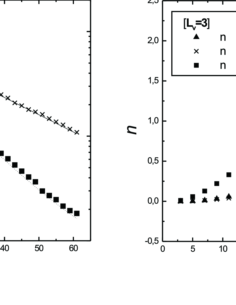
Figure 5: a) Probability of a trivial knot $P_{tk}(L_{h};p)$ on a strip of width $L_{v}=3$ and length $L_{h}$ for concentration of impurities $p=0.05,0.1$; b) Complexity $n(L_{h};p)$ of a daughter (quasi)knots on a strip of width $L_{v}=3$ and length $L_{h}$ for concentration of impurities $p=0.05$ under condition that the parent knot $L_{t}=3L_{h}$ (triangles) and $L_{t}=2L_{h}+1$ (crosses) is trivial. For comparison, the complexity of a random U–knots $n(L_{h};p)$ on a strip $3\times L_{h}$ is plotted by squares.

In the last case the averaging is performed over $10\times 3000$ samples. One sees from Fig.5a that probability of a trivial knot formation exponentially decays with the length of the strip. The results of corresponding approximations are plotted in Fig.5a by lines. The same results of approximation for $L_{v}=5$ are enclosed in the Table 2.

Table 2

$L_{v}=3$
$p$	$P_{tr}(L_{h};p)$
$0.05$	$1.049(4)\exp(-0.03720(15)\times L_{h})$
$0.1$	$0.957(22)\exp(-0.0673(5)\times L_{h})$

$L_{v}=5$
$p$	$P_{tr}(L_{h};p)$
$0.05$	$1.155(7)\exp(-0.0794(3)\times L_{h})$
$0.1$	$1.2305(22)\exp(-0.1568(11)\times L_{h})$

It follows from the Table 2 that the probability of a trivial knot formation (i.e. of knots with $n=0$) is exponentially small for sufficiently long strips.

IV.2 Conditional distribution (“Brownian Bridge”)

Let us investigate now the topological correlations of parts of a trivial knot. Namely, consider a trivial (”parent”) knot, generated on a strip of width $L_{v}$ and length $L_{t}$. Cut a part of the strip of length $L_{h}$ ($0<L_{h}<L_{t}$) and close the remaining open tails. In such a way we get the new (”daughter”) knot of the same width $L_{v}$ but of shorter length $L_{h}$. In Fig.2a,b the parent and a daughter knots are shown. All lattice dimensions $L_{v},\;L_{t},\;L_{h}$ are taken to be odd.

We pay the main attention to the following problem. How the fact that the parent knot $L_{v}\times L_{t}$ is trivial is reflected in the topological properties of the daughter (quasi)knot $L_{v}\times L_{h}$? We consider two cases $L_{h}=L_{t}/3$ and $L_{h}=(L_{t}-1)/2$. To be more precise, we define the conditional probability that daughter (quasi)knot is trivial and find its mean complexity under the condition that the parent knot is trivial.

The problem under consideration is typical for the theory of random walks. Namely, in the theory of Markovian chains the conditional probability i.e. the so called ”Brownian Bridge” (BB) has repeatedly studied. The investigation of statistics of BB supposes in first turn the determination of the probability $P({\bf x},t|{\bf 0},T)$ that a random walk begins at the point ${\bf x}={\bf 0}$, visits the point ${\bf x}$ at some intermediate moment $0<t<T$ and returns to the initial point ${\bf x}={\bf 0}$ at the moment $T$. The same question has been investigated for BB on the graphs of free groups, on the Riemann surfaces nesin1 ; bougerol and for the products of random matrices of groups $PSL(2,{\sf Z\kern-4.49997ptZ})$ nesin2 and $PSL(n,{\sf Z\kern-4.49997ptZ})$ letch .

Its easy to understand, that topological problem under consideration can be naturally interpreted in terms of BB. As it has been mentioned above (for details see grne_alg ; vasne ) the power $n$ of Jones–Kauffman polynomial invariants defines the scale in the space of topological states of knots. That allow us to compare knots and to talk about their respective ”complexity” or ”simplicity”. Take a phase space $\Omega$ of all topological states of knots. Select from $\Omega$ the subset $\Omega_{n=0}$ of knots with $n=0$. Cut a part (say, one half, or one third) of each knot in the subset $\Omega_{n=0}$, close the open ends and investigate the topological properties of resulting knots. Just such situation was qualitatively investigated in grne_alg , where the authors have formulated the ”crumpled globule” (CG) concept on the basis of qualitative conjectures. The CG–hypothesis states the following. If the whole knot is trivial, then the topological state of each its finite part is almost trivial. Later on we formulate this statement in more rigorous terms and confirm its by results of our numerical computations.

IV.2.1 The mean complexity of a (quasi)knot

We consider the strips of width $L_{v}=3$. The concentration of ”impurities” is set to $p=0.05$. The averaging is performed over $3\times 10^{4}$ selected trivial knots. The mean complexities $n(L_{h})$ of ”daughter” knots on the strips $L_{v}\times L_{h}$ for $L_{v}=3$ under the condition that corresponding ”parent” knots on the strips $L_{t}=3L_{h}$ (triangles) and $L_{t}=2L_{h}+1$ (crosses) are trivial, are shown on Fig.5b. We have compared the complexity of BB (daughter) knots (triangles, crosses) with the unconditional (U) complexity of random knots (squares). Its easy to see, that complexity of the BB–knots is sufficiently smaller than the complexity of U–knots. The functional dependence of $n$ upon $L_{h}$ for BB–knots shall be discussed later.

IV.2.2 The probability of the trivial (quasi)knot

Here we investigate the probability that a daughter knot on the strip $L_{v}\times L_{h}$ is trivial under condition that it is a part of a trivial (parent) knot on the strip $L_{t}=2L_{h}+1$. Results for $L_{h}=3,5,7$ are shown in Fig.4b by crosses, squares and triangles respectively. The unconditional probabilities of formation of the trivial knot are plotted for $L_{h}=3,5,7$ by lines in Fig.4b. As expected, the probability of a (quasi)knot to be trivial becomes essentially higher under imposing condition for this (quasi)knot to be a part of the trivial knot.

IV.3 Lyapunov exponents and the knot complexity

We are interested in the functional dependence of the complexity $n$ of the BB (daughter) knot upon the lattice length $L_{h}$ for fixed width $L_{v}$. The direct investigation of this question meets some technical difficulties and to avoid them we shall use some properties of product of random matrices. According to vasne for a knot on the strip of width $L_{v}=3$ we introduce the matrices

$$\begin{array}[]{cc}P=(1+x)x^{-\frac{1}{2}}\left(\begin{array}[]{cc}-x^{\frac{1}{2}}&0\\ (1+x)^{-1}x^{\frac{1}{2}}&x^{-\frac{1}{2}}\\ \end{array}\right)&R=x^{\frac{1}{2}}\left(\begin{array}[]{cc}-x^{\frac{1}{2}}&-(x+1)x^{-\frac{1}{2}}\\ 0&x^{-\frac{1}{2}}\end{array}\right)\\ \rule{0.0pt}{31.29802pt}P^{*}=(1+x)x^{-\frac{1}{2}}\left(\begin{array}[]{cc}-x^{-\frac{1}{2}}&0\\ (1+x)^{-1}x^{\frac{1}{2}}&x^{\frac{1}{2}}\\ \end{array}\right)&R^{*}=x^{\frac{1}{2}}\left(\begin{array}[]{cc}-x^{-\frac{1}{2}}&-(x^{-1}+1)x^{-\frac{1}{2}}\\ 0&x^{\frac{1}{2}}\end{array}\right)\end{array}$$ (7)

corresponding to ferro– and antiferromagnetic bonds as shown in Fig.3d.

The polynomial knot invariants can be expressed as the product of these matrices. For example, the resulting matrix $A$ of the knot, shown in Fig.3a corresponding to the bond arrangement in Fig.3b,c is:

$$A=PR^{*}PP^{*}RP^{*}PR^{*}PPR^{*}PP^{*}RP^{*}$$ (8)

From vasne it follows, that the Jones polynome for the knot on the strip of width $L_{v}=3$ reads:

$$f_{K}(x)=(1+x)^{-N_{p}-1}\left(-\sqrt{x}\right)^{N_{p}+1+N_{b}}\left((x+x^{-1}+2)a_{12}+(x+x^{-1}+2)^{2}a_{22}\right)$$ (9)

where $a_{12}$ and $a_{22}$ are the elements of the last column of the product $A$ of the transfer matrices.

Let us investigate the relationship between the knot complexity $n$ and the logarithm of the highest eigenvalue $n_{\lambda}$ of the product of transfer matrices. Note that when calculating the knot invariant, one has the trivial prefactor $d=(1+x)^{-N_{p}-1}\left(-\sqrt{x}\right)^{N_{p}+1+N_{b}}$, where $N_{p}=(L_{v}+1)(L_{h}+1)/2$ is a number of Potts spin components and $N_{b}=\sum\limits_{i,j}b_{i,j}$ is a sum over all $b_{i,j}$. So it is convenient to add $\log d$ to the largest power $n_{\lambda}$ and introduce the modified value $\tilde{n}_{\lambda}=n_{\lambda}-(N_{p}+1-N_{b})/2$. For the strip on the lattice of width $L_{v}=3$ and concentration of impurities $p=0.05$ the data for $\tilde{n}_{\lambda}$ in the interval $L_{h}\in[20,60]$ is well approximated by the linear function

$$\tilde{n}_{\lambda}(L_{h})=-1.16(2)+0.0741(6)\times L_{h}$$ (10)

This results establishes the linear dependence of the knot complexity upon $L_{h}$.

We have also computed $\tilde{n}_{\lambda}$ for BB–knot of length $L_{h}$ for $L_{t}=3L_{h}$ and $L_{t}=2L_{h}+1$. The corresponding results are plotted in Fig.6a.

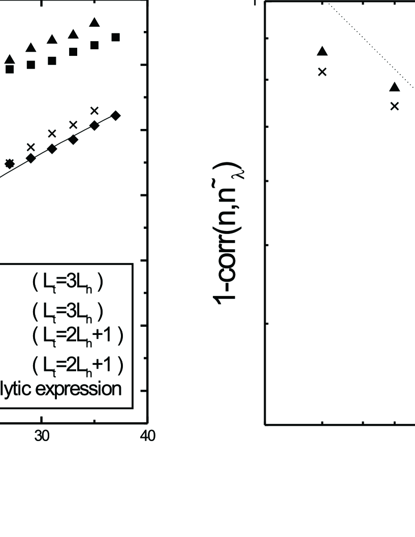
Figure 6: a) Power of the Jones–Kauffman polynomial invariant $n$ and the exponent of the maximal eigenvalue of the product $\tilde{n}_{\lambda}$ of transfer matrices for BB–knots $L_{t}=3L_{h}$ and $L_{t}=2L_{h}+1$; b) Correlation function ${\rm corr}(n,\tilde{n}_{\lambda})$ as a function of $L_{h}$ for BB–knots $p=0.05,0.1$, $L_{v}=3$.

These results are well approximated by the square-root function shown in Fig.6a by a line:

$$\tilde{n}_{\lambda}(L_{h})=-1.74(3)+0.300(22)\times L_{h}^{0.498(16)}$$ (11)

We have plotted in Fig.6a the data for $n$ for comparison as well.

The information about the behavior of the knot complexity we could obtain analyzing the the correlation coefficient of the knot complexity $n$ and the logarithm of the modified highest eigenvalue $\tilde{n}_{\lambda}$:

$${\rm corr}(n,\tilde{n}_{\lambda})=\frac{\left<n\,\tilde{n}_{\lambda}\right>-\left<n\right>\left<\tilde{n}_{\lambda}\right>}{\sqrt{(\left<n^{2}\right>-\left<n\right>^{2})(\left<\tilde{n}_{\lambda}^{2}\right>-\left<\tilde{n}_{\lambda}\right>^{2})}}$$ (12)

The difference $1-{\rm corr}(n,\tilde{n}_{\lambda})$ is shown in Fig.6b (the function $1.57L^{-0.4}$ is added for comparison). We see, that the correlation between $\tilde{n}_{\lambda}$ and $n$ approaches to $1$ as $L_{h}$ tends to infinity. This behavior allows us to conclude that the averaged knot complexity $n$ has the same dependence upon $L_{h}$ as the mean logarithm of the modified highest eigenvalue $\tilde{n}_{\lambda}$.

V Conclusions

The correlation between $n$ and $\tilde{n}_{\lambda}$ established in the previous section permits us to consider the distribution of Lyapunov exponents for products of transfer matrices instead of distribution of largest power of polynomial invariant.

Qualitatively the behavior (11) can be understood by considering the limiting distribution of Lyapunov exponents of first $m$ matrices in a product of $N$ random unimodular $2\times 2$ matrices under the condition, that the product as a whole equals the unit matrix. The explicit analysis of the problem has been developed in nesin2 . In nesin2 the authors studied the distribution of the Lyapunov exponent $\delta$ of first $m=cN\;(0<c<1)$ matrices in the product of $N$ non-commuting $PSL(2,{\sf I\kern-1.49994ptR})$–matrices whose elements are independently distributed in some finite interval under the condition of the Brownian Bridge (i.e. under the condition that the whole product equals the unit matrix). The exponent $\delta$ obeys for $N\gg 1$ the following asymptotic behavior:

$$\delta\sim\sqrt{N}$$ (13)

(compare to (11)). Without the Brownian Bridge condition (i.e. for ”open” chains of matrices) the standard Fürstenberg result fuerst_tut has been reproduced

$$\delta\sim N$$ (14)

In order to clarify the behavior (13) we restrict ourselves mainly with a qualitative consideration. The ”Brownian Bridge” problem for Markov chain of $N$ identically distributed noncommutative random matrices may be reformulated in terms of a random walk in the space of the constant negative curvature. Now it is well known nesin1 ; bougerol ; letch that BB condition to return to the initial point ”kills” the influence of the curvature. The limiting distribution function turns to be the Gaussian with zero mean. This fact can be illustrated by the following simple computation.

Consider the random walk in a space of the constant negative curvature $\gamma=-1$ (the Lobachevsky space) with the metric $ds^{2}=d\mu^{2}+\sinh^{2}\mu\,d\Phi^{2}$, where $d\Phi^{2}$ is a square of distance increment in the space of angles. The probability of a path to start from the point $\mu=0$ and to end at the time moment $t$ in a particular point located at distance $\mu$ from the origin in the Lobachevsky space is well known:

$$P(\mu,t)=\frac{e^{-t}}{8\sqrt{(\pi t)^{3}}}\frac{\mu}{\sinh\mu}\exp\left(-\frac{\mu^{2}}{4t}\right)$$ (15)

(the diffusion coefficient $D$ is set to 1). For the first time Eq.(15) was obtained in karp_gervas . Respectively, the probability to find a walker at time moment $t$ in some point at a distance $\mu$ from the origin is:

$${\cal P}(\mu,t)=P(\mu,t){\cal N}_{s}(\mu)$$ (16)

where ${\cal N}_{s}(\mu)=\sinh^{2}\mu$ is an area of the sphere of radius $\mu$ in the Lobachevsky space.

The difference between $P$ and ${\cal P}$ is vanishing in the Euclidean space, but becomes crucial in the non–Euclidean geometry. By using definition of the Brownian Bridge we can easily calculate the conditional probability that the random walk starting and finishing at $\mu=0$ after $t$ first steps visits some point at distance $\mu$ from the origin in the Lobachevsky space. This probability for $N\to\infty$ reads:

$${\cal P}(\mu,t|0,N)=\frac{P(\mu,t)P(\mu,N-t)\sinh^{2}\mu}{P(0,t)}=\frac{N^{3/2}}{8\pi t^{3/2}(N-t)^{3/2}}\mu^{2}\exp\left\{-\frac{\mu^{2}}{4}\left(\frac{1}{t}+\frac{1}{N-t}\right)\right\}$$ (17)

Thus, we arrive at the Gaussian distribution with zero mean.

The behavior (17) found for the random walks on the Riemann surface of the constant negative curvature has the straightforward relation to the conditional distribution of Lyapunov exponents of the products of noncommutative random matrices. The Lobachevsky space $H$ may be identified with the noncommutative group $SL(2,{\kern 1.00006pt{\raise 2.0236pt\hbox{$\scriptscriptstyle|$}}\kern-3.99994pt{\sf C}})/SO(3)$. Let us take the ”Brownian Bridge” on ${\cal H}=SL(2,{\kern 1.00006pt{\raise 2.0236pt\hbox{$\scriptscriptstyle|$}}\kern-3.99994pt{\sf C}})/SO(3)$. Namely consider the product of $N$ random matrices $\widehat{\cal M}_{k}\in{\cal H}\;(0\leq k\leq N)$ under the condition that the product $A=\prod_{k=1}^{N}\widehat{\cal M}_{k}$ is identical to the unit matrix. We are interested in the distribution of Lyapunov exponents $\delta$ for the first $m$ matrices in the product $A$. The stochastic recursion relation for the vector $\displaystyle{\bf W}_{k}$ reads:

$${\bf W}_{k+1}=\widehat{\cal M}_{k}{\bf W}_{k};\qquad{\bf W}_{0}={\rm const}$$ (18)

where ${\cal M}_{k}\in{\cal H}$ for all $k\in[0,N]$. The ”Brownian Bridge” condition means that

$${\bf W}_{N}={\bf W}_{0}$$ (19)

Consider for simplicity the case when each matrix in the product is close to the unit one:

$$\widehat{\cal M}_{k}=1+\widehat{M}_{k};\qquad\mbox{norm}[\widehat{M}_{k}]\ll 1$$ (20)

The discrete dynamical equation (18) under the condition (20) may be replaced by the differential equation. Its stationary distribution is defined by an appropriate Fokker–Plank equation for the random walk in the Lobachevsky space. The distribution of the Lyapunov exponent $\delta$ for the conditional product $A$ of random matrices is given by (17). So, under the conditions (19) and (20) for $\delta$ we have recovered the usual Gaussian distribution. Hence the mean value $\left<\delta_{m}\right>$ of the Lyapunov exponent of any first $m=cN$ ($c={\rm const}$, $0<c<1$) matrices has the square–root dependence on $N$ ($N\gg 1$): $\left<\delta_{m}\right>\sim\sqrt{N}$.

This statement can be reformulated in topological terms. As it has been shown, the correlation between the knot complexity and the Lyapunov exponent tends to 1 for $L_{h}\to\infty$. Thus we can conclude that the typical complexity $n$ of topological Jones–Kauffman invariant of a daughter quasi–knot, obtained by cutting a part $N=L_{v}\times L_{h}$ of a trivial parent knot of size $L_{v}\times L_{t}$, scales as

$$n\sim\sqrt{N}\sim\sqrt{L_{h}}$$

for $N\gg 1$. Contrary, for a random knot of size $N=L_{v}\times L_{h}$ without the Brownian Bridge condition the complexity scales as $n\sim N\sim L_{h}$ (see vasne ) in agreement with the Fürstenberg theorem fuerst_tut ).

Therefore the relative complexity $\frac{n}{N}$ of a daughter quasi–knot, which is a part of a trivial knot, tends to 0:

$$\lim_{N\to\infty}\frac{n}{N}=\lim_{N\to\infty}\frac{{\rm const}\,\sqrt{N}}{N}=0$$

The Figs.4b and 5b confirm our statement. Actually, the mean complexity of a BB–knot is smaller than the typical complexity of a random knot of the same size without the BB–condition. The probability for a part of a trivial knot to be also trivial is sufficiently higher than the corresponding unconditional probability for a random knot (of the same size) to be trivial—see Fig.4b. Thus we directly validate the hypothesis that the topological state of any daughter quasi–knot, which is a part of a trivial parent knot, is almost trivial. Hence, the parts of a polymer chain in the crumpled globule are practically unknotted in a broad range of scales.

The investigation carried out above could be considered as an indirect verification of a hypothesis expressed in nechaev concerning the possibility to formulate some topological problems of collapsed polymer chains in terms of path integrals over trajectories with prescribed fractal dimension and without any topological ingredients. Namely, in ensemble of collapsed polymer chains the essential fraction of trajectories has the fractal dimension of dense packing state $D_{f}=d$ ($d$ is the space dimensionality). Conversely there is a reason to assume that almost all paths in ensemble of trajectories with fractal dimension $D_{f}=d$ (where $d\leq 3$) are topologically isomorphic to knots, close to trivial.

The problem of calculation of distribution for closed polymer chain with topological constraints can be expressed as an integral over the set $\Omega$ of closed paths with fixed topological invariant:

$$Z=\int\limits_{\Omega}D\{r\}e^{-H}=\int\ldots\int D\{r\}e^{-H}\Delta[n],$$ (21)

where $D\{r\}e^{-H}$ is the integration with the Wiener measure and $\Delta[n]$ extracts paths with the value of the power $n$ of the topological Jones–Kauffman invariant equal to zero.

If our assumption is right, the integration over $\Omega$ in (21) can be replaced by the integration over all paths without any topological restriction but with special ”fractal” measure $D_{f}\{r\}e^{-H_{f}}$:

$$Z=\int\ldots\int D_{f}\{r\}e^{-H_{f}}$$ (22)

The usual Wiener measure $D\{r\}e^{-H}$ is concentrated on the trajectories with the fractal dimension $D_{f}=2$. We suppose, that for description of statistics of ring unknotted polymer chains the measure $D_{f}\{r\}e^{-H_{f}}$ with fractal dimension $D_{f}=d$ ($d\leq 3$) should be used.

Acknowledgments

The work is partially supported by the RFBR grant 00-15-99302. O.A.V thanks the laboratory LPTMS (Université Paris Sud, Orsay) for hospitality. We appreciate the useful comments of J.-L. Jacobsen concerning the realization of numerical algorithm used in our work. The authors are grateful to Supercomputer Center (RAN) for available computational resources.

References

- (1) I.M. Lifshitz, JETP, 55 2408 (1968)
- (2) I.M. Lifshits, A.Yu. Grosberg, A.R. Khokhlov, Rev. Mod. Phys., 50 683 (1978)
- (3) A.Yu. Grosberg, A.R. Khokhlov, Statistical physics of macromolecules (New York: AIP Press, 1994)
- (4) A.Yu. Grosberg, S.K. Nechaev, E.I. Shakhnovich, J.Phys.(Paris), 49 2095 (1988)
- (5) B.B. Mandelbrot The Fractal Geometry of Nature, (San Francisco: Freeeman, 1982)
- (6) B. Chu, Q. Ying, A. Grosberg, Macromolecules, 28 180 (1995)
- (7) W.L. Nachlis, R.P. Kambour, W.J. McKnight, Polymer, 39 3643 (1994)
- (8) J. Ma, J.E. Straub, E.I. Shakhnovich, J. Chem. Phys., 103 2615 (1995)
- (9) V.F.R. Jones, Bull. Am. Math. Soc., 12 103 (1985)
- (10) L.H. Kauffman, Topology, 26 395 (1987)
- (11) F.Y. Wu, J. Knot Theory Ramific., 1 47 (1992)
- (12) A.Yu. Grosberg, S. Nechaev, J. Phys. (A): Math. Gen., 25 4659 (1992); A.Yu. Grosberg, S. Nechaev, Europhys. Lett., 20 603 (1992)
- (13) O.A. Vasilyev, S.K. Nechaev, JETP, 93 1119 (2001)
- (14) I.M. Lifshitz, A.Yu. Grosberg, JETP, 65 2399 (1973)
- (15) L.B. Koralov, S.K. Nechaev, Ya.G. Sinai, Prob. Theory Appl., 38 331 (1993) (in Rusian)
- (16) P. Bougerol, Probab. Th. Rel. Fields 78 193 (1988)
- (17) S. Nechaev, Ya.G. Sinai, Bol. Soc. Bras. Mat., 21 121 (1991)
- (18) A.V. Letchikov, Russ. Math. Surv., 51 49 (1996)
- (19) H. Fürstenberg, Trans. Amer. Math. Soc., 198 377 (1963); V.N. Tatubalin, Prob. Theory Appl., 10 15 (1965), Prob. Theory Appl., 13 65 (1968)
- (20) M.E. Gerzenshtein, V.B. Vasilyev, Prob. Theory Appl., 4 424 (1959); F.I. Karpelevich, V.N. Tatubalin, M.G. Shur, Prob. Theory Appl., 4 432 (1959)
- (21) A.Yu. Grosberg, S.K. Nechaev, Polymer topology, Adv. Polym. Sci., 106 1, in Polymer Characteristics, (Springer: Berlin, 1993); S.K. Nechaev, Statistics of Knots and Entangled Random walks, (WSPC: Singapore, 1996)