Nonlinear waves in a cylindrical Bose-Einstein condensate

Abstract

We present a complete calculation of solitary waves propagating in a steady state with constant velocity $v$ along a cigar-shaped Bose-Einstein trap approximated as infinitely-long cylindrical. For sufficiently weak couplings (densities) the main features of the calculated solitons could be captured by effective one-dimensional (1D) models. However, for stronger couplings of practical interest, the relevant solitary waves are found to be hybrids of quasi-1D solitons and 3D vortex rings. An interesting hierarchy of vortex rings occurs as the effective coupling constant is increased through a sequence of critical values. The energy-momentum dispersion of the above structures is shown to exhibit characteristics similar to a mode proposed sometime ago by Lieb within a strictly 1D model, as well as some rotonlike features.

I Introduction

Solitary waves that may occur in a Bose-Einstein Condensate (BEC) have been traditionally discussed in terms of the classical Gross-Pitaevskii (GP) model which is appropriate for the description of weakly correlated systems dalfovo . For instance, a simple soliton was obtained by Tsuzuki tsuzuki in a homogeneous 1D model, while Zakharov and Shabat zakharov developed inverse-scattering techniques for the study of multisolitons. Interestingly, the elementary soliton proved to be relevant for an accurate semiclassical description kulish ; ishikawa of an intriguing mode proposed earlier by Lieb lieb in a full quantum treatment of a 1D Bose gas based on the Bethe Ansatz lieb2 .

The above developments had long remained purely theoretical because of the absence of a physical realization of a strictly 1D Bose gas. Nevertheless, the picture has significantly changed with the recent observation of similar coherent structures in confined BECs of alkali-metal atoms burger ; denschlag . The very method of experimental production of solitary waves (phase imprinting) was inspired by the analytical structure of the 1D soliton, while various effective 1D models have been developed for their theoretical investigation perez ; jackson ; muryshev ; feder ; dikande ; muryshev2 ; salasnich . On the other hand, the actual stability of the theoretically predicted 1D solitary waves should be questioned within the proper 3D environment of realistic traps muryshev ; feder ; dikande . An important step in that direction was the experimental observation anderson that a dark soliton initially created in a finite trap eventually decays into vortex rings, as is also predicted by a numerical solution of the corresponding initial-value problem in a 3D classical GP model feder .

Therefore, it is important to carry out a calculation of potential nonlinear modes without a priori assumptions about their effective dimensionality. One could envisage a picture in which the actual solitary waves are hybrids of quasi-1D solitons and 3D vortex rings. It is the aim of the present paper to make the above claim precise by calculating solitary waves that propagate along a cylindrical trap in a steady state with constant velocity $v$. Our approach was motivated by the calculation of vortex rings in a homogeneous BEC due to Jones and Roberts jones1 and a similar calculation of semitopological solitons in planar ferromagnets semi .

We have already described the main result of this work in a recent short communication komineas but a substantial elaboration is necessary in order to appreciate its full significance. Thus the problem is formulated in Sec. II where we also present a brief but complete recalculation of the ground state and the corresponding linear (Bogoliubov) modes for comparison. A detailed calculation of nonlinear modes is given in Sec. III and the main conclusions are summarized in Sec. IV.

II Formulation and linear modes

The physical picture that we have in mind is a slight idealization of the experiment in Ref. burger . Thus we consider a cigar-shaped trap filled with atoms of mass $m$. The transverse confinement frequency is denoted by $\omega_{\bot}$ and the corresponding oscillator length by $a_{\bot}\!=\!(\hbar/m\omega_{\bot})^{1/2}$. The longitudinal confinement frequency $\omega_{\|}$ is assumed to be much smaller than $\omega_{\bot}$, hence we make the approximation of an infinitely-long cylindrical trap with $\omega_{\|}\!=\!0$. Accordingly, complete specification of the system requires as input the average linear density $\nu$ which is the number of atoms per unit length of the cylindrical trap. Finally, we consider the two dimensionless combinations of parameters:

$$\gamma=\nu a\,,\quad\gamma_{\bot}=\nu a_{\bot}\,,$$ (1)

where $a$ is the scattering length related to the coupling constant as usual by $U_{0}\!=\!4\pi\hbar^{2}a/m$.

Now, in the actual experiment of Ref. burger , the trap is filled with ⁸⁷Rb atoms, the transverse frequency is chosen as $\omega_{\bot}\!=\!2\pi\times 425$ Hz, the oscillator length is calculated to be $a_{\bot}\!\approx\!0.5\mu m$, and the estimated linear density lies in the range $\nu\!>0.1\,\hbox{atoms}/\hbox{\AA}$. Also taking into account a scattering length $a\!\approx\!50\,\hbox{\AA}$, the dimensionless parameters (1) take values in $\gamma\!>\!5$ and $\gamma_{\bot}\!>\!5\times 10^{2}$. In fact, our subsequent calculations will be carried out for a much wider range of the above parameters. Therefore, apart from the idealization of a cylindrical trap, our results are fairly realistic and could be applied to a number of cases of experimental interest.

It is useful to introduce rationalized units through the rescalings

$$t\!\to\!\frac{t}{\omega_{\bot}},\quad{{\hbox{\bf r}}}\!\to\!a_{\bot}{{\hbox{\bf r}}},\quad\Psi\!\to\!\frac{\nu^{1/2}}{a_{\bot}}\,\Psi.$$ (2)

The energy functional extended to include a chemical potential is then given by

$$W=\frac{1}{2}\int{\left[\bm{\nabla}\Psi^{*}\bm{\nabla}\Psi+\rho^{2}\,\Psi^{*}\Psi+g(\Psi^{*}\Psi)^{2}-2\mu\,\Psi^{*}\Psi\right]\,dV},$$ (3)

where $g\!=\!4\pi\gamma$ and $\rho^{2}\!=\!x^{2}+y^{2}$. Eq. (3) yields energy $W$ in units of $\gamma_{\bot}(\hbar\omega_{\bot})$ whereas the chemical potential $\mu$ is measured in units of $\hbar\omega_{\bot}$. The corresponding rationalized equation of motion reads

$$i\frac{\partial\Psi}{\partial t}=-\frac{1}{2}\Delta\Psi+\frac{1}{2}\rho^{2}\Psi+g(\Psi^{*}\Psi)\Psi-\mu\Psi\,,$$ (4)

and depends only on the dimensionless coupling constant $\gamma$, because $g\!=\!4\pi\gamma$ and the chemical potential $\mu\!=\!\mu(\gamma)$ is fixed by the requirement that the system carry in its ground state a definite average linear density $\nu$.

Figure 1: Radial dependence of the ground-state wave function for four representative values of the dimensionless coupling constant $\gamma\!=\!0,1,10$ and 100. The corresponding values of the chemical potential were calculated to be $\mu\!=\!1,\,2.2571,\,6.4324$, and 20.0431, in units of $\hbar\omega_{\bot}$. The inset compares the accurate numerical solution (solid line) with the TF approximation (7) (dotted line) for the strong coupling $\gamma\!=\!100$. Distance is measured in units of $a_{\bot}$.

An important first step is thus to obtain accurate information about the ground-state wave function $\Psi\!=\!\Psi_{0}(\rho)$ which is normalized according to

$$\int_{0}^{\infty}{2\pi\rho\,d\rho\,|\Psi_{0}|^{2}}=1\,,$$ (5)

to conform with our choice of rationalized units. The wave function $\Psi_{0}(\rho)$ is numerically calculated as the minimum of the energy functional, under the constraint (5) that fixes the chemical potential $\mu(\gamma)$, by a variant of a relaxation algorithm dalfovo2 . Explicit results are illustrated in Fig. 1 for some typical values of $\gamma$ where we also quote the corresponding values of the chemical potential.

The preceding numerical determination of the ground state will provide the basis for all subsequent calculations. However, it is worth mentioning here some limiting cases where the ground state is known analytically. At $\gamma\!=\!0$,

$$\Psi_{0}=\frac{1}{\sqrt{\pi}}\,e^{-\rho^{2}/2}\,,$$ (6)

and the chemical potential degenerates to $\mu\!=\!1$. In the opposite limit, $\gamma\!\gg\!1$, one may use the Thomas-Fermi (TF) approximation baym

$$\Psi_{0}=\left[\frac{2}{\pi R_{\bot}^{2}}\left(1-\frac{\rho^{2}}{R_{\bot}^{2}}\right)\right]^{1/2}$$ (7)

for $0\!\leq\!\rho\!\leq\!R_{\bot}\!=\!2\gamma^{1/4}$, and $\Psi_{0}\!=\!0$ for $\rho\!>\!R_{\bot}$. The chemical potential is given accordingly by $\mu\!\approx\!2\,\gamma^{1/2}$. A comparison with the accurate numerical solution is shown in the inset of Fig. 1 for $\gamma\!=\!100$. In fact, as we shall see shortly, the TF approximation provides a reasonable description of some quantities of physical interest even for $\gamma\!\sim\!1$.

We will also need some information from the linear (Bogoliubov) modes which have already been calculated in the literature to varying degree of completeness zaremba ; stringari ; fedichev . Here we employ a numerical algorithm of our own briefly described as follows. Equation (4) is linearized by inserting $\Psi\!=\!\Psi_{0}+f+i\chi$ where $\Psi_{0}(\rho)$ is the calculated ground-state wave function while $f\!=\!f({{\hbox{\bf r}}},t)$ and $\chi\!=\!\chi({{\hbox{\bf r}}},t)$ are real functions that account for small fluctuations around the ground state. It is somewhat more convenient to use the linear combinations $a\!=\!f+\chi$ and $b\!=\!f-\chi$ which satisfy the linearized equations

$$\frac{\partial}{\partial t}\left(\begin{array}[]{c}a\\ b\end{array}\right)=M\left(\begin{array}[]{c}a\\ b\end{array}\right)\,,\quad M\equiv\left(\begin{array}[]{cc}-V&-D\\ D&V\end{array}\right)$$ (8)

where

$$V=g\Psi_{0}^{2},\quad D=-\frac{1}{2}\Delta+\frac{1}{2}\rho^{2}+2\,V-\mu\,.$$ (9)

Our task is then to calculate the spectrum of the differential operator $M$ whose eigenvalues are purely imaginary and come in pairs $\pm i\omega$ where $\omega$ is the sought after physical frequency.

We restrict attention to axially-symmetric waves that propagate along the $z$ axis with wave number $q$. The Laplace operator is then replaced by

$$\Delta=\frac{\partial^{2}}{\partial\rho^{2}}+\frac{1}{\rho}\frac{\partial}{\partial\rho}-q^{2}$$ (10)

and the amplitudes $a$ and $b$ may be assumed to depend only on the radial distance $\rho$. A finite-matrix approximation of the operator $M$ is obtained by expanding both $a$ and $b$ in terms of a basis set of non-orthogonal Gaussian wave packets with randomly chosen oscillator lengths papspathis . It is also prudent to enlarge the basis set by including the ground-state wave function $\Psi_{0}(\rho)$ itself, in order to directly account for the zero (Goldstone) mode associated with the number symmetry. The resulting algorithm is then quite efficient and provides stable approximations of the low-lying eigenvalues even if we include a small number of basis elements.

Figure 2: The lowest branch in the Bogoliubov spectrum for four representative values of the dimensionless coupling constant $\gamma\!=\!0,1,10$ and 100. The frequency $\omega$ is measured in units of $\omega_{\bot}$ and the wave number $q$ in units of $1/a_{\bot}$. The corresponding values of the speed of sound were calculated to be $c\!=\!0,\,0.95,\,1.77$, and 3.17, in units of $a_{\bot}\omega_{\bot}$.

In Fig. 2 we present explicit results for the lowest eigenfrequency $\omega\!=\!\omega(q)$ for the same set of coupling constants as in Fig. 1. At $\gamma\!=\!0$, $\omega(q)$ reduces to the free-particle quadratic dispersion $\omega\!=\!q^{2}/2$, as expected. At nonzero $\gamma$, the dispersion becomes linear near the origin, $\omega\!\approx\!c|q|$, where $c$ is the speed of sound for which explicit values are also quoted in Fig. 2. Finally, we note that our results are in apparent agreement with the Bogoliubov dispersion calculated earlier within the TF approximation zaremba ; stringari as well as numerically fedichev – even though a different parameterization of the spectrum was employed in the latter reference.

Figure 3: Speed of sound $c$ in units of $a_{\bot}\omega_{\bot}$ as a function of the dimensionless coupling constant $\gamma$. Open circles stand for our numerical data, the solid line for the TF asymptote of Eq. (11), and the dotted line for the weak-coupling asymptote of Eq. (12).

The speed of sound is a quantity of special physical interest and will also play an important role in the theoretical development of Sec. III. Hence we have carried out a calculation for a wider set of coupling constants and the results are summarized in Fig. 3. It is interesting that our accurate numerical results are consistent with the TF approximation zaremba ; stringari ; kavoulakis

$$c\approx\gamma^{1/4}$$ (11)

even for values of $\gamma$ as low as 1, where the error is about 5%, whereas the error is reduced to less than 1% for $\gamma\!\buildrel>\over{\sim}\!10$. This fact is especially important because Eq. (11) was employed for the analysis of experimental data andrews . The relative accuracy of this approximation progressively deteriorates in the region $\gamma\!<\!1$, but a new asymptote, namely

$$c\approx(2\gamma)^{1/2}\,,$$ (12)

was predicted to be reached for sufficiently weak couplings jackson . The weak-coupling approximation (12) is actually consistent with our numerical data for $\gamma\!<\!1/4$, as is shown in the inset of Fig. 3. However, we should add that the linear part of the Bogoliubov dispersion becomes very narrow in this region of couplings.

III Nonlinear waves

We now turn to the calculation of axially-symmetric solitary waves traveling along the $z$ axis in a steady state with constant velocity $v$. These are described by a wave function of the form $\Psi\!=\!\Psi(\rho,\xi)$, with $\xi\!=\!z-vt$, which is inserted in Eq. (4) to yield the stationary differential equation

$$-iv\,\frac{\partial\Psi}{\partial\xi} = -\frac{1}{2}\Delta\Psi+\frac{1}{2}\rho^{2}\Psi+g(\Psi^{*}\Psi)\Psi-\mu\Psi\,,$$ (13)

$$\Delta = \frac{\partial^{2}}{\partial\rho^{2}}+\frac{1}{\rho}\frac{\partial}{\partial\rho}+\frac{\partial^{2}}{\partial\xi^{2}}\,.$$

The wave function must vanish in the limit $\rho\to\infty$, thanks to the transverse confinement, while the condition

$$\lim_{\xi\to\pm\infty}|\Psi(\rho,\xi)|=|\Psi_{0}(\rho)|$$ (14)

enforces the requirement that the local particle density coincide asymptotically with that of the ground state calculated in Sec. II. But the phase of the wave function is not fixed a priori at spatial infinity except for a mild restriction implied by the von Neumann boundary condition

$$\lim_{\xi\to\pm\infty}\frac{\partial\Psi}{\partial\xi}=0$$ (15)

adopted in our numerical calculation. Our task is then to find concrete solutions of Eq. (13) that satisfy the boundary conditions just described.

An important check of the numerical calculation is provided by the virial relation

$$v\,{\cal P}=\int{\left[\frac{1}{2}\frac{\partial\Psi^{*}}{\partial\xi}\frac{\partial\Psi}{\partial\xi}+\rho^{2}\,\Psi^{*}\Psi+\frac{g}{2}(\Psi^{*}\Psi)^{2}-\mu\,\Psi^{*}\Psi\right]dV}\,,$$ (16)

obtained by standard scaling arguments semi . Here ${\cal P}$ is the linear momentum given by the usual definition

$${\cal P}=\frac{1}{2i}\,\int{\left(\Psi^{*}\frac{\partial\Psi}{\partial z}-\frac{\partial\Psi^{*}}{\partial z}\Psi\right)\;dV}=\int{n\,\frac{\partial\phi}{\partial z}\;dV},$$ (17)

and is measured in units of $\hbar\nu\!=\!\gamma_{\bot}(\hbar/a_{\bot})$. In the second step of Eq. (17) we employ hydrodynamic variables defined from

$$\Psi=\sqrt{n}\,e^{i\phi}\,,$$ (18)

where $n\!=\!|\Psi|^{2}$ is the local particle density and the phase $\phi$ may be used to construct the velocity field ${{\hbox{\bf u}}}=\bm{\nabla}\phi$.

Numerical solutions of Eq. (13) are obtained by an iterative Newton-Raphson algorithm jones1 ; semi briefly described as follows. Suppose that $\Psi\!=\!\Psi_{\rm in}$ is an initial rough guess for the solution at some velocity $v$. We then insert in Eq. (13) the configuration $\Psi_{\rm out}\!=\!\Psi_{\rm in}+X$ and keep terms that are at most linear in the amplitude $X$. Thus we derive an inhomogeneous differential equation of the form $LX\!=\!Y$ where the linear operator $L$ and the source $Y$ are both calculated in terms of $\Psi_{\rm in}$. We solve this linear system for $X\!=\!L^{-1}Y$ to obtain $\Psi_{\rm out}\!=\!\Psi_{\rm in}+L^{-1}Y$ which is used as input for the next iteration until convergence is achieved at some specified level of accuracy. The procedure is repeated by incrementing the velocity to a different value, typically in steps of $\delta v\!=\!\pm 0.01$, using as input the converged configuration obtained at the preceding value of the velocity. Therefore, the main numerical burden consists of constructing a finite-matrix lattice approximation of the linear operator $L$ which is then inverted by standard routines appropriate for sparse linear systems.

The Newton-Raphson algorithm typically converges after a few iterations and the final configuration is independent of the specific choice $\Psi_{\rm in}$. But it is also clear that the algorithm will not converge for most choices of $\Psi_{\rm in}$. Hence it is important to invoke an educated guess for the input configuration provided by the product Ansatz:

$$\Psi_{\rm in}=[c_{1}-i\,c_{2}\tanh(c_{3}\xi)]\,\Psi_{0}(\rho)$$ (19)

which capitalizes on the analytically known solitary wave in the homogeneous 1D model tsuzuki ; zakharov and the ground-state configuration $\Psi_{0}(\rho)$ numerically calculated in Sec. II. The constants $c_{1},c_{2}$ and $c_{3}$ are definite functions of the velocity $v$ within the strictly 1D model, but such precise relations need not be invoked for our current purposes except for the normalization condition $c_{1}^{2}+c_{2}^{2}\!=\!1$ that is necessary to enforce the boundary condition (14). In other words, the above constants are treated here as trial parameters until we achieve convergence for a specific velocity $v$. A corrolary of the preceding discussion is that the converged configuration does not depend on the precise choice of those parameters, and it is certainly not in the form of a product Ansatz often employed for the derivation of effective 1D models jackson ; salasnich . Finally, we note that the Ansatz (19) satisfies the parity relations

$$\hbox{Re}\,\Psi(\rho,\xi)=\hbox{Re}\,\Psi(\rho,-\xi),\quad\hbox{Im}\,\Psi(\rho,\xi)=-\hbox{Im}\,\Psi(\rho,-\xi)$$ (20)

which are compatible with Eq. (13) and are actually satisfied by all solutions constructed in the present paper.

Figure 4: Solitary wave for $\gamma\!=\!1$ and two representative values of the velocity: $v\!=\!c/2$ (I) and $v\!=\!0$ (II). We display the radial dependence of the real and the imaginary part of the wave function for various positive values of $\xi$ in steps of $\delta\xi\!=\!0.1$. The corresponding results for negative $\xi$ are obtained through the parity relations (20).

We begin with the special case of the relatively weak coupling $\gamma\!=\!1$ for which the speed of sound was calculated to be $c\!=\!0.95$ in Sec. II. The simplest possibility is to first attempt to derive a static ($v\!=\!0$) soliton starting with the input configuration (19) applied for, say, $c_{1}\!=\!0$ and $c_{2}\!=\!1\!=\!c_{3}$. Indeed, the algorithm quickly converges to a wave function with a nontrivial imaginary part but vanishing real part. The velocity is then incremented to positive values in steps of $\delta v\!=\!0.01$ and the corresponding wave functions acquire also a nontrivial real part. The process may be continued until the velocity $v$ approaches the speed of sound $c$ beyond which the solitary wave ceases to exist. An equivalent sequence of solitary waves with velocities in the range $-c\!<\!v\!\leq 0$ is obtained either by starting again with the $v\!=\!0$ soliton and pushing it to negative velocities or, simply, by taking the complex conjugate of the wave function calculated for $0\!\leq v\!<\!c$, since

$$v\to-v,\quad\Psi\to\Psi^{*}\,,$$ (21)

is an obvious symmetry of Eq. (13). A detailed illustration of the calculated solitary wave function is given in Fig. 4 for two representative values of the velocity: $v\!=\!c/2$ and $v\!=\!0$.

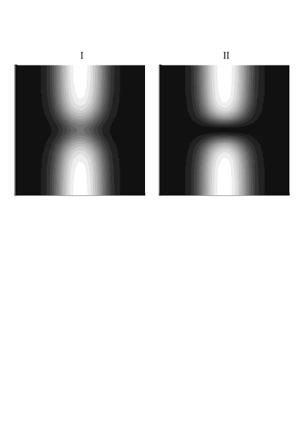
Figure 5: Contour levels of the local particle density $n\!=\!|\Psi|^{2}$ for $\gamma\!=\!1$, in a plane that contains the $z$ axis and cuts across the cylindrical trap. The complete 3D picture may be envisaged by simple revolution around the $z$ axis. Regions with high particle density are bright while regions with zero density are black. The two special cases considered are the same as in Fig. 4.

A partial but more transparent illustration is given in Fig. 5 which depicts the level contours of the local particle density $n\!=\!|\Psi|^{2}$ for the two special cases considered in Fig. 4. In words, the calculated solitary wave is a mild soundlike disturbance of the ground state when $|v|$ approaches the speed of sound $c$, while it becomes an increasingly dark soliton with decreasing $|v|$ and reduces to a completely dark (black) soliton at $v\!=\!0$.

It is now important to calculate the energy-momentum dispersion of the solitary wave. The excitation energy is defined as

$$E=W-W_{0}$$ (22)

where both $W$ and $W_{0}$ are calculated from Eq. (3) applied for the solitary wave $\Psi(\rho,\xi)$ and the ground state $\Psi_{0}(\rho)$, respectively. The presence of the chemical potential in Eq. (3) provides the compensation that is necessary to compare energies of states with the same number of particles. Similarly, the relevant physical momentum is not the linear momentum ${\cal P}$ of Eq. (17) but the impulse $Q$ defined in a manner analogous to the case of a homogeneous gas kulish ; ishikawa ,

$$Q = \int{(n-n_{0})\,\frac{\partial\phi}{\partial z}\,dV}={\cal P}-\delta\phi\,,$$ (23)

$$\delta\phi \equiv \int_{0}^{\infty}{2\pi\rho\,d\rho\;n_{0}(\rho)[\phi(\rho,z\!=\!\infty)-\phi(\rho,z\!=\!-\infty)]}\,,$$

where $n_{0}\!=\!|\Psi_{0}(\rho)|^{2}$ is the ground-state particle density and $\delta\phi$ is now the weighted average of the phase difference between the two ends of the trap. The delicate distinction between linear momentum and impulse has been the subject of discussion in practically all treatments of classical fluid dynamics batchelor ; saffman and continues to play an important role in the dynamics of superfluids jones1 . Here we simply postulate the validity of the definition of impulse in Eq. (23) and note that the corresponding group-velocity relation

$$v=\frac{dE}{dQ}$$ (24)

is satisfied to an excellent accuracy in our numerical calculation and thus provides a highly nontrivial check of consistency. In turn, the virial relation (16) is verified using the standard definition of the linear momentum ${\cal P}$ in Eq. (17), as expected. We finally note that the same phase difference $\delta\phi$ which is important for experimental production of solitary waves through phase imprinting burger ; denschlag is also crucial for the calculation of the impulse.

Figure 6: Energy $E$ in units of $\gamma_{\bot}(\hbar\omega_{\bot})$ versus impulse $Q$ in units of $\gamma_{\bot}(\hbar/a_{\bot})$ for $\gamma\!=\!1$. The solid line corresponds to the complete sequence of solitary waves discussed in the text, and the dotted line to the $\gamma\!=\!1$ Bogoliubov dispersion of Fig. 2 adjusted to current units. Symbols I and II correspond to the two special cases of the solitary wave illustrated in Figs. 4 and 5.

The dispersion $E\!=\!E(Q)$ calculated for the complete sequence of solitary waves with velocities in the range $-c\!<\!v\!<\!c$ is illustrated in Fig. 6. The apparent $2\pi$ periodicity seems surprising, but occured also in the original calculation of a similar mode by Lieb lieb within a full quantum treatment of a 1D Bose gas interacting via a $\delta$-function potential. The Lieb mode was later rederived by a fairly accurate semiclassical approximation based on the elementary solitary wave of the 1D classical GP model kulish ; ishikawa .

Lieb further argued that the corresponding Bogoliubov mode is no more elementary and thus proposed an intriguing dual interpretation of the excitation spectrum. It should be noted that the dispersions of the two modes exhibit the same linear dependence at low momenta, $E\!\approx\!c|Q|$, where $c$ is the speed of sound, but significant differences arise at finite momenta. The differences are especially pronounced in the current calculation within a cylindrical trap. Specifically, let us assume an average linear density $\nu\!=\!0.02\,\hbox{atoms}/\hbox{\AA}$ which leads to $\gamma\!=\!\nu a\!=\!1$ and $\gamma_{\bot}\!=\!\nu a_{\bot}\!=\!10^{2}$. If we then adjust the $\gamma\!=\!1$ Bogoliubov dispersion of Fig. 2 to the units employed in Fig. 6, the two dispersions are seen to diverge very quickly at the scale of Fig. 6. In other words, Bogoliubov and Lieb modes operate at rather different energy and momentum scales in a realistic trap.

To summarize the preceding accurate calculation for $\gamma\!=\!1$, the solitary wave is essentially quasi-1D in this weak-coupling region and its main features are indeed captured by an effective 1D model jackson2 . However, all cases of actual experimental interest burger ; denschlag ; anderson are characterized by significantly larger values of the effective coupling where quasi-1D solitons are expected to be unstable muryshev ; feder . In particular, Ref. muryshev suggests that a critical coupling occurs in a cylindrical trap when $n_{\rm max}U_{0}/\hbar\omega_{\bot}\!=\!2.4$, where $n_{\rm max}$ is the maximum local particle density in the ground state of the trap. If we tentatively assume that the TF approximation (7) can be trusted at the anticipated critical coupling, the above criticality condition reads $2\gamma^{1/2}\!=\!2.4$ where $\gamma$ is the dimensionless effective coupling constant defined in Eq. (1). The root of this equation $\gamma\!=\!\gamma_{c}\!=\!1.44$ provides a critical coupling $\gamma_{c}$ above which quasi-1D solitons are predicted to be unstable jackson2 .

In fact, our numerical calculation suggests that the quasi-1D nature of the solitary wave is completely lost at a higher critical coupling, namely for $\gamma\!>\!\gamma_{1}\!\approx\!3.9$. The emerging new picture is clear at $\gamma\!=\!10$ which is the special case described in our recent short communication komineas . This case is reanalyzed and further extended in the continuation of the present paper.

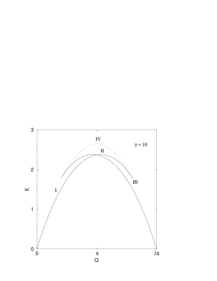
Figure 7: Energy $E$ in units of $\gamma_{\bot}(\hbar\omega_{\bot})$ versus impulse $Q$ in units of $\gamma_{\bot}(\hbar/a_{\bot})$ for $\gamma\!=\!10$. The solid line corresponds to the fundamental sequence of vortex rings discussed in the text, and the dotted line to the auxiliary sequence that contains the black soliton (point IV).

It is natural to begin again with the calculation of a static ($v\!=\!0$) soliton obtained by using the input configuration (19) with $c_{1}\!=\!0,c_{2}\!=\!1$ and practically any $c_{3}$. We then increment the velocity to both positive and negative values in steps of $\delta v\!=\!\pm 0.01$ to yield a sequence of solitary waves which now display two surprising features. First, a ringlike structure develops for $\gamma\!=\!10$ that was not present at $\gamma\!=\!1$. Second, the above sequence exists only over the limited velocity range $-v_{1}\!<\!v\!<\!v_{1}$ where $v_{1}\!=\!0.84\!=\!0.47\,c$ and $c\!=\!1.77$ is the speed of sound calculated in Sec. II for $\gamma\!=\!10$. The existence of a critical velocity $v_{1}$ also becomes apparent in the energy-momentum dispersion of the above sequence depicted by a dotted line in Fig. 7. This portion of the dispersion is symmetric around $Q\!=\!\pi$, where it achieves a maximum, but remains open ended at two critical points that correspond to $v\!=\!\pm v_{1}$.

It is thus not surprising that an independent sequence of solitary waves with lower energy exists for $\gamma\!=\!10$. Indeed, we return to the input configuration (19) but now target a solution with velocity in the range $v_{1}\!<\!v\!<\!c$. After some experimentation a solution is obtained for, say, $v\!=\!1.5$ if we choose the trial parameters $c_{1}\!=\!0.2$, $c_{2}\!=\!0.98$ and $c_{3}\!=\!3$. Having thus obtained a specific solution for $v\!=\!1.5$ the algorithm is iterated forward and backwards in steps of $\delta v\!=\!\pm 0.01$ to obtain an entirely new sequence of solitary waves in the velocity range $-v_{1}\!<\!v\!<\!c$, and a corresponding sequence for $-c\!<\!v\!<\!v_{1}$ through the symmetry relation (21). Here $v_{1}$ is the same critical velocity encountered in the preceding paragraph, as is also apparent in the calculated energy-momentum dispersions which are depicted by solid lines in Fig. 7 and join the previously calculated dotted line through cusps that correspond to $v\!=\!\pm v_{1}$.

Figure 8: Solitary wave for $\gamma\!=\!10$ and a representative value of the velocity $v\!=\!c/2$. We show the radial dependence of the real and the imaginary part of the wave function for various values of $\xi$ in steps of $\delta\xi\!=\!0.1$. The corresponding results for negative $\xi$ are obtained through the parity relations (20).

Figure 9: Radial dependence of the local particle density $n\!=\!|\Psi|^{2}$ for $\gamma\!=\!10$, using the same conventions for the $\xi$ dependence as in Fig. 8. The four special cases considered correspond to the four representative points I, II, III, and IV along the energy-momentum dispersion of Fig. 7.

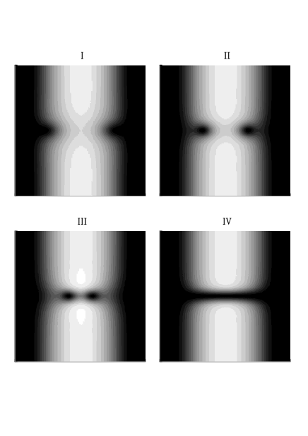
Figure 10: Contour levels of the local particle density $n\!=\!|\Psi|^{2}$ for $\gamma\!=\!10$, in a plane that contains the $z$ axis and cuts across the cylindrical trap. The complete 3D picture may be envisaged by simple revolution around the $z$ axis. Regions with high particle density are bright while regions with zero density are black. The four special cases considered are the same as in Fig. 9.

Hence we turn to a description of the detailed nature of this new sequence of solitary waves. For values of the velocity near the speed of sound $c$, the calculated soliton appears again as a mild soundlike disturbance of the ground state. The dominant features of the solitary wave are pronounced as the velocity is decreased to lower values and become reasonably apparent for $v\!=\!c/2$ that corresponds to point I in the dispersion of Fig.7. The wave function is completely illustrated through its real and imaginary parts in Fig. 8. An important new feature emerges by comparison with the corresponding case at $\gamma\!=\!1$ illustrated in frame I of Fig. 4. Both the real and the imaginary part at the center of the soliton ($\xi\!=\!0$) now vanish for a specific radius $R\!=\!2.8$, thus a vortex ring is beginning to emerge. A partial but more transparent illustration is given in Fig. 9 where we depict the radial dependence of the local particle density $n\!=\!|\Psi|^{2}$ for various values of $\xi$. Again it is clear that the density near the center of the soliton ($\xi\!=\!0$) vanishes on a ring with a relatively large radius $R\!=\!2.8\,$. The features of the vortex ring become completely apparent, and its radius is tightened, as we proceed to smaller values of the velocity. A notable special case is the static ($v\!=\!0$) vortex ring with radius $R\!=\!1.8$ illustrated in frame II of Fig. 9, which is far from being a black soliton. The corresponding point II in Fig. 7 is thus a new local maximum of the energy-momentum dispersion, which is clearly distinguished from the local maximum at point IV that corresponds to the static black soliton discussed earlier in the text.

One would think that pushing the velocity $v$ to negative values would somehow retrace the calculated sequence of vortex rings backwards. In fact, our algorithm continues to converge to vortex rings of smaller radii until the critical velocity $-v_{1}$ is encountered where the ring achieves its minimum radius $R_{\rm min}\!=\!0.8$ and ceases to exist for smaller values of $v$. The terminal state at $v\!=\!-v_{1}$ is illustrated in frame III of Fig. 9. We have thus described a sequence of solitary waves that consists of bonafide 3D vortex rings and does not contain a black soliton. The corresponding branch in the energy-momentum dispersion of Fig. 7 is labeled by points I, II, and III that stand for the special cases $v\!=\!c/2,0$, and $-v_{1}$. As mentioned already, an equivalent sequence of solitary waves exists in the range $-c\!<\!v\!<\!v_{1}$ and leads to a dispersion curve in Fig. 7 that is mirror symmetric to the branch (I,II,III) around $Q\!=\!\pi$.

To complete the description for $\gamma\!=\!10$ we must briefly return to the auxiliary sequence of solitary waves associated with the portion of the dispersion that is depicted by a dotted line in Fig. 7. As one moves from point III to point IV, the ringlike structure is more or less preserved at constant radius $R\!=\!R_{\rm min}\!=\!0.8$. Nevertheless, the detailed features of the vortex ring are tamed at small velocities and completely disappear for $v\!=\!0$ to yield a black soliton at point IV.

We thus essentially conclude our description of solitary waves for $\gamma\!=\!10$ by schematically summarizing our main results in Fig. 10. Yet some of the elements of the preceding discussion are sufficiently surprising to deserve closer attention. For example, simple inspection of Fig. 7 reveals that the group velocity becomes negative in the region (II,III) or, equivalently, the impulse is opposite to the group velocity. This rotonlike behavior is consistent with the Onsager-Feynman view of a roton as the ghost of a vanished vortex ring donnelly because the calculated radius of the vortex ring is monotonically decreasing along the fundamental (I,II,III) sequence. A full-scale roton would develop if the terminal point III were an inflection point beyond which the group velocity begins to rise again. Actually, this is exactly what happens as one moves away from point III along the upper branch in Fig. 7, but this “roton” portion of the dispersion now appears in a strange location by comparison to the usual situation in liquid helium donnelly . On the other hand, the black soliton at the stationary point IV is indeed the ghost of a vanished vortex ring, as explained in the preceding paragraph.

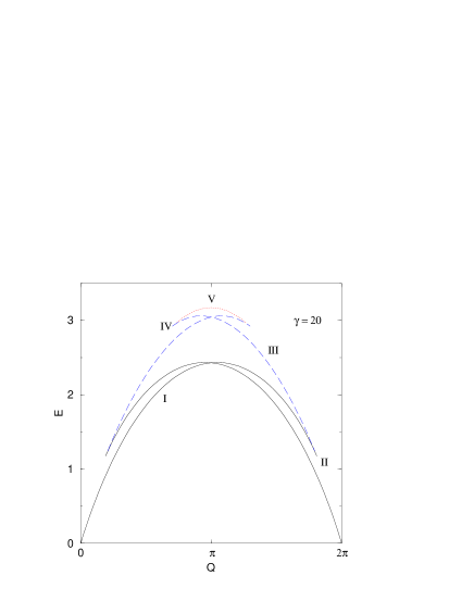
Figure 11: Energy $E$ in units of $\gamma_{\bot}(\hbar\omega_{\bot})$ versus impulse $Q$ in units of $\gamma_{\bot}(\hbar/a_{\bot})$ for $\gamma\!=\!20$. The solid lines correspond to the fundamental single-ring sequence, the dashed lines to the double-ring sequence, and the dotted line to the auxiliary sequence that contains a black soliton (point V).

It is also interesting to question how the picture just described evolves with increasing values of the dimensionless coupling constant $\gamma$ which is the only parameter that enters the rationalized GP equation. Our numerical calculations have revealed yet another critical coupling $\gamma_{2}\!\approx\!12$, in the sense that new flavor arises for $\gamma\!>\!\gamma_{2}$. The structure of the solitary waves in this new regime becomes sufficiently clear for $\gamma\!=\!20$ and is best summarized by the calculated energy-momentum dispersion shown in Fig. 11. Apart from mirror symmetry, the dispersion now exhibits two cusps that correspond to two critical velocities $v_{1}\!=\!1.35\!=\!0.64c$ and $v_{2}\!=\!0.48\!=\!0.23\,c$, where $c\!=\!2.1$ is the speed of sound calculated for $\gamma\!=\!20$ as in Sec. II.

Figure 12: Radial dependence of the local particle density $n\!=\!|\Psi|^{2}$ for $\gamma\!=\!20$. The four special cases considered correspond to points I, II, III, and IV along the energy-momentum dispersion of Fig. 11. Point V in the above dispersion in not illustrated here because it corresponds to a black soliton similar to that shown earlier in frame IV of Fig. 9.

The nature of the solitary waves associated with the various branches in the dispersion of Fig. 11 is very briefly described with the aid of Fig. 12. Thus we consider the sequence of five characteristic points (I,II,…,V) that roughly cover half of the dispersion, the other half being obtained by the mirror symmetry (21). The lowest branch (I,II) corresponds to single vortex rings with velocities in the range $c\!>\!v\!>\!-v_{1}$, as in the case $\gamma\!=\!10$. Again the ring achieves its minimum radius at the critical velocity $v\!=\!-v_{1}$ (point II). The new element for $\gamma\!=\!20$ is the intermediate branch (II,III,IV) that corresponds to double rings with velocities in the range $v_{2}\!>\!v\!>\!-v_{1}$. The second ring is first created at the flanks of the trap and comes closest to the original ring at the new critical velocity $v\!=\!v_{2}$ (point IV). This double-ring configuration is more or less preserved along the upper branch (IV,V), with velocities in the range $v_{2}\!>\!v\!>\!0$, but gradually fades away to become a black soliton at $v\!=\!0$ (point V).

While the numerical calculation becomes increasingly more difficult for larger values of $\gamma$, it is clear that a sequence of critical couplings $\gamma_{1},\gamma_{2},\ldots$ exists and leads to a hierarchy of axisymmetric vortex rings. The single-ring solution associated with the lowest branch of the spectrum is a robust feature for all $\gamma\!>\!\gamma_{1}\!\approx\!3.9$ and is likely stable to all perturbations. But it is possible that the multiple-ring configurations associated with the higher branches are unstable to non-axisymmetric perturbations. In this respect, one should recall that the solitary wave that corresponds to the upper branch in the original calculation of Jones and Roberts jones1 within the homogeneous GP model was later argued to be unstable jones2 .

However, we should emphasize that the vortex rings constructed here differ significantly from the Jones-Roberts (JR) vortex ring that provided the basic motivation for the present work. As with ordinary smoke rings in fluid dynamics, the JR ring can never be static thanks to a virial relation of the type (16) that prevents finite-energy solutions with $v\!=\!0$ in the homogeneous GP model. As a result, the radius of the vortex ring grows to infinity at low velocity. This picture is completely rearranged in a cylindrical trap because the occurrence of slow vortex rings with large radius is restricted by the boundaries of the trap. Instead, vortex rings are predicted to nucleate at the flanks of the trap as soundlike pulses with high velocity approaching the speed of sound $c$, and their radius actually decreases with decreasing velocity. In particular, it is now possible to obtain static ($v\!=\!0$) vortex rings of finite radius that are no longer contradicted by the virial relation (16). The structure of the energy-momentum dispersions calculated throughout the present paper clearly reflects the substantial restructuring of vortex rings within a cylindrical trap.

It is then natural to question whether or not there exists a limit in which the JR vortex ring is recovered. One should expect that this may happen when the bulk healing length $L\!=\!(na)^{-1/2}$ is significantly smaller than the transverse oscillator length $a_{\bot}$. This limit is translated into large values of $\gamma\!=\!\nu a$ which is the only dimensionless parameter that enters the rationalized GP equation. Now, our discussion earlier in this section suggests an increasingly complicated hierarchical structure in the strong-coupling limit rather that a simple JR soliton. A logical conclusion is that a JR vortex ring somehow created within the bulk will sooner or later sense the boundaries of the cylindrical trap. It will thus either directly dissipate into sound waves, or reorganize itself to conform with one or more of the presently calculated vortex rings possibly after ejecting some amount of radiation in the form of sound waves.

The preceding remarks indicate a certain non-uniformity that is inherent in the approximation of the cigar-shaped trap by an infinitely-long cylindrical trap. The same phenomenon is also apparent in the calculation of linear modes in Sec. II. For instance, neither one of the two asymptotes for the speed of sound quoted in Eqs. (11) and (12) approaches the well-known Bogoliubov speed in a homogeneous Bose gas jackson . But a non-uniformity of this type is not a reason to doubt that a sufficiently elongated trap can be approximated by an infinitely-long cylindrical trap.

IV Conclusion

We have thus presented a complete 3D calculation of solitary waves in a cylindrical Bose-Einstein condensate. In all cases considered there exists a nontrivial phase difference $\delta\phi$ that is reminiscent of strictly 1D solitons tsuzuki ; zakharov and is important for their experimental production through phase imprinting burger ; denschlag .

Nevertheless, the detailed structure of the solitary waves depends crucially on the strength of the dimensionless effective coupling constant $\gamma$. Quasi-1D solitons occur only in the weak-coupling region $\gamma\!<\!\gamma_{1}\!\approx\!3.9$ where some of our accurate numerical results could be approximated through effective 1D models jackson2 . But a sufficiently strong coupling or density is necessary in order to pronounce the special features of a condensate. It is thus not surprising that the effective coupling in experiments performed so far lies in the region $\gamma\!>\!\gamma_{1}$ where the nature of the theoretically predicted solitary waves changes drastically.

For $\gamma\!>\!\gamma_{1}$ solitary waves are still characterized by a nontrivial phase difference $\delta\phi$ between the two ends of the trap but are otherwise 3D vortex rings. This finding is consistent with a recent experiment anderson and a corresponding theoretical analysis feder in finite traps. The main mathematical advantage of the approximation of a sufficiently elongated trap by an infinitely-long cylindrical trap is that vortex rings can then be calculated in a steady state propagating with a constant velocity $v$. It is thus possible to carry out a detailed study of the soliton profile as a function of the effective coupling constant $\gamma$ and the velocity $v$, as is done in the present paper.

An interesting by-product of the above idealization is that a soliton is characterized by a definite energy-momentum dispersion. The calculated dispersion is found to be the direct analog of the Lieb mode lieb in the weak-coupling region and acquires interesting rotonlike features for stronger couplings. Perhaps such a dispersion can be measured by a combination of phase imprinting burger ; denschlag with Bragg spectroscopy recently employed for the detection of the usual Bogoliubov mode stamper ; ozeri . In this respect, one should keep in mind that Bogoliubov and Lieb modes operate at different energy and momentum scales in a realistic trap. This fact becomes evident by the different sets of physical units employed for the Bogoliubov mode in Fig. 2 and the Lieb mode in, say, Fig. 6. The difference is accounted for by the second dimensionless coupling $\gamma_{\bot}\!=\!\nu a_{\bot}$ in Eq. (1) which is much stronger than $\gamma\!=\!\nu a$ because $\gamma_{\bot}/\gamma\!=\!a_{\bot}/a\!\sim\!10^{2}$.

- (1) F. Dalfovo, S. Giorgini, L.P. Pitaevskii, and S. Stringari, Rev. Mod. Phys. 71, 463 (1999).
- (2) T. Tsuzuki, J. Low Temp. Phys. 4, 441 (1971).
- (3) V.E. Zakharov and A.B. Sabat, Sov. Phys. JETP 37, 823 (1973).
- (4) P.P. Kulish, S.V. Manakov, and L.D. Faddeev, Theor. Math. Phys. 28, 615 (1976).
- (5) M. Ishikawa and H. Takayama, J. Phys. Soc. Japan 49, 1242 (1980).
- (6) E.H. Lieb, Phys. Rev. 130, 1616 (1963).
- (7) E.H. Lieb and W. Liniger, Phys. Rev. 130, 1605 (1963).
- (8) S. Burger, K. Bongs, S. Dettmer, W. Ertmer, K. Sengstock, A. Sanpera, G.V. Shlyapnikov, and M. Lewenstein, Phys. Rev. Lett. 83, 5198 (1999).
- (9) J. Denschlag, J. E. Simsarian, D. L. Feder, Charles W. Clark, L.A. Collins, J. Gubizolles, L. Deng, E.W. Hagley, K. Helmerson, W.P. Reinhardt, S.L. Rolston, B.I. Schneider, and W.D. Phillips, Science 287, 97 (2000).
- (10) V.M. Pérez-Garcia, H. Michinel, and H. Herrero, Phys. Rev. A 57, 3837 (1998).
- (11) A.D. Jackson, G.M. Kavoulakis, and C.J. Pethick, Phys. Rev. A 58, 2417 (1998).
- (12) A.E. Muryshev, H.B. van Linden van den Heuvell, and G.V. Shlyapnikov, Phys. Rev. A 60, R2665 (1999).
- (13) D.L. Feder, M.S. Pindzola, L.A. Collins, B.I. Schneider, and C.W. Clark, Phys. Rev. A 62, 053606 (2000).
- (14) A.M. Dikande, e-print cond-mat/0111418 .
- (15) A.E. Muryshev, G.V. Shlyapnikov, W. Ertmer, K. Sengstock, and M. Lewenstein, e-print cond-mat/0111506 .
- (16) L. Salasnich, A. Parola, and L. Reatto, e-print cond-mat/0201395 .
- (17) B.P. Anderson, P.C. Haljan, C.A. Regal, D.L. Feder, L.A. Collins, C.W. Clark, and E.A. Cornell, Phys. Rev. Lett. 86, 2926 (2001).
- (18) C.A. Jones and P.H. Roberts, J. Phys. A: Math. Gen. 15, 2599 (1982).
- (19) N. Papanicolaou and P.N. Spathis, Nonlinearity 12, 285 (1999).
- (20) S. Komineas and N. Papanicolaou, e-print cond-mat/0202182 .
- (21) F. Dalfovo and S. Stringari, Phys. Rev. A 53, 2477 (1996).
- (22) G. Baym and C.J. Pethick, Phys. Rev. Lett. 76, 6 (1996).
- (23) E. Zaremba, Phys. Rev. A 57, 518 (1998).
- (24) S. Stringari, Phys. Rev. A 58, 2385 (1998).
- (25) P.O. Fedichev and G.V. Shlyapnikov, Phys. Rev. A 63, 045601 (2001).
- (26) N. Papanicolaou and P.N. Spathis, J. Phys. G 11, 149 (1985).
- (27) G.M. Kavoulakis and C.J. Pethick, Phys. Rev. A 58, 1563 (1998).
- (28) M.R. Andrews, D.M. Kurn, H.-J. Miesner, D.S. Durfee, C.G. Townsend, S. Inouye, and W. Ketterle, Phys. Rev. Lett. 79, 553 (1997); ibid 80, 2967 (1998).
- (29) G.K. Batchelor, An Introduction to Fluid Dynamics (Cambridge University Press, 1967).
- (30) P.G. Saffman, Vortex Dynamics (Cambridge University Press, 1992).
- (31) A.D. Jackson and G.M. Kavoulakis, e-print cond-mat/0202178 .
- (32) R.J. Donnelly, Quantized Vortices in Helium II (Cambridge University Press, 1991).
- (33) C.A. Jones, S.J. Putterman, and P.H. Roberts, J. Phys. A: Math. Gen. 19, 2991 (1986).
- (34) D.M. Stamper-Kurn, A.P. Chikkatur, A. Görlitz, S. Inouye, S. Gupta, D.E. Pritchard, and W. Ketterle, Phys. Rev. Lett. 83, 2876 (1999).
- (35) R. Ozeri, J. Steinhauer, N. Katz, and N. Davidson, e-print cond-mat/0112496 .