Fronts with a Growth Cutoff but Speed Higher than $v^{*}$

Abstract

Fronts, propagating into an unstable state $\phi=0$, whose asymptotic speed $v_{\text{as}}$ is equal to the linear spreading speed $v^{*}$ of infinitesimal perturbations about that state (so-called pulled fronts) are very sensitive to changes in the growth rate $f(\phi)$ for $\phi\ll 1$. It was recently found that with a small cutoff, $f(\phi)=0$ for $\phi<\varepsilon$, $v_{\text{as}}$ converges to $v^{*}$ very slowly from below, as $\ln^{-2}\varepsilon$. Here we show that with such a cutoff and a small enhancement of the growth rate for small $\phi$ behind it, one can have $v_{\text{as}}>v^{*}$, even in the limit $\varepsilon\to 0$. The effect is confirmed in a stochastic lattice model simulation where the growth rules for a few particles per site are accordingly modified.

Pulled fronts are those fronts that propagate into a linearly unstable state, and whose asymptotic front speed $v_{\text{as}}$ equals the linear spreading speed $v^{*}$ of infinitesimal perturbations about the unstable state bj ; vs2 ; ebert . The name pulled front refers to the picture that in the leading edge of these fronts, the perturbation about the unstable state grows and spreads with speed $v^{*}$, while the rest of the front gets “pulled along” by the leading edge. That this notion is not merely an intuitive picture but can be turned into a mathematically precise analysis is illustrated by the recent derivation of exact results for the general power law convergence of the front speed to the asymptotic value $v^{*}$ ebert . Fronts which propagate into a linearly unstable state and whose asymptotic speed $v_{\text{as}}>v^{*}$ are refered to as pushed, as it is the nonlinear growth in the region behind the leading edge that pushes their front speed to higher values. If the state is not linearly unstable, then $v^{*}$ is trivially zero; in such cases the front propagation is always dominated by the nonlinear growth in the front region itself, and hence fronts in this case are in a sense “pushed” too.

For the field $\phi(x,t)$, the dynamics of fronts that we consider in this paper is given by the usual nonlinear diffusion equation

$$\frac{\partial\phi}{\partial t}\,=\,\frac{\partial^{2}\phi}{\partial x^{2}}\,+\,f(\phi)\,.$$ (1)

In the standard case, the growth function $f(\phi)$ has the form $f(\phi)=\phi-\phi^{n}$, with $n>1$. Equation (1) has two stationary states for $\phi(x,t)$: $\phi(x,t)=0$ and $\phi(x,t)=1$. Of these, $\phi(x,t)=1$ is stable and $\phi(x,t)=0$ is unstable. The asymptotic speed of (pulled) fronts propagating from $\phi(x,t)=1$ into $\phi(x,t)=0$ in Eq. (1) is $v^{*}=2$.

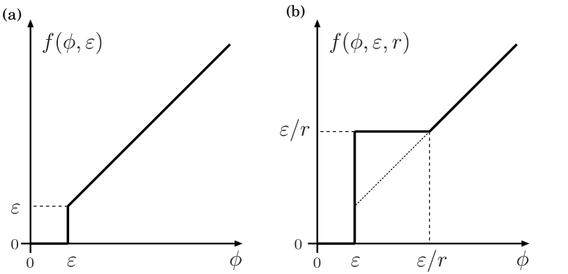
Figure 1: (a) Shape of the function $f(\phi,\varepsilon)$ used by Brunet and Derrida to study the effect of a finite particle cutoff in the growth rate on the front speed. (b) The growth function $f(\phi,\varepsilon,r)$ (thick line) we analyze in this paper. In both cases we have kept only the linear term of $f(\phi)$ to plot the graphs, since $\varepsilon\ll 1$, so that the nonlinear terms in $f$ are much smaller than the linear terms.

The sensitivity of pulled fronts to the precise dynamics for small perturbations about the unstable state has recently surfaced in a remarkable way bd . Often, in equations like (1), the field $\phi(x,t)$ is the density of particles in a continuum description. If one then considers fronts in stochastic particle model versions of (1), the linear growth term in $f(\phi)$ implies that for small particle density, the rate at which new particles are created is proportional to the density itself. Brunet and Derrida bd were the first to realize the fact that for new particles to be created in any given realization, the density must be at least one “quantum” of particle density strong, and that this provides a natural lower cutoff for the growth that strongly affects the front speed. Indeed, to mimic this effect, they considered a deterministic front of the type in Eq. (1) with $n=3$, and by hand introduced a cutoff of the type sketched in Fig. 1a in the growth function at $\phi=\varepsilon\ll 1$. In this paper, we denote their growth function by $f(\phi,\varepsilon)\equiv[\phi-\phi^{3}]\,\Theta(\phi-\varepsilon)$ where $\Theta$ is the unit step function. For small $\varepsilon$, the asymptotic front speed $v_{\text{as}}(\varepsilon)$ was then found to be bd

$$v_{\text{as}}(\varepsilon)\,\simeq\,v^{*}\,-\,\frac{\pi^{2}}{(\ln\varepsilon)^{2}}+\cdots\,.$$ (2)

Brunet and Derrida subsequently identified $\varepsilon$ with $1/N$, where $N$ is the average number of particles at the saturation state of the front, corresponding to the stable state $\phi(x,t)=1$ of the density field. The slow logarithmic convergence to the asymptotic front speed from below as a function of $N$, implied by Eq. (2), has been confirmed in various studies of stochastic lattice models bd ; breuer ; vanzon ; kns ; levine ; PvS . Note that for $\phi<\varepsilon$, the growth function $f$ vanishes, and as a result, strictly speaking, the state $\phi=0$ is not linearly unstable; hence fronts in this model are always weakly pushed for any nonzero value of $\varepsilon$ deb2 .

In this paper, we demonstrate an even more surprising aspect of the sensitivity to small changes in the growth function $f$ of the “pulled” fronts, that we have at $\varepsilon=0$: if $f$ is sufficiently enhanced in a range of $\phi$ of the order of $\varepsilon$, the asymptotic front speed $v_{\text{as}}$ can become larger than $v^{*}$ and not converge to $v^{*}$ as $\varepsilon\to 0$. For fluctuating fronts, this implies that if the stochastic growth rates for small occupation densities $n_{i}$ are somewhwat enhanced over a linear behavior $\sim n_{i}$, then such stochastic fronts may move faster than $v^{*}$ and never converge to their naive mean field limit for $N\to\infty$. This effect may be of relevance for the coarse-grained field theory for DLA, as it is empirically known to be essential to modify the growth function for small cluster densities brener .

We now discuss our results first, and then summarize their derivation.

To be specific, we consider the nonlinear diffusion equation (1) with the growth function sketched in Fig. 1b,

$$f(\phi,\varepsilon,r)\, = \,f(\phi,\varepsilon)\quad\mbox{for}\,\,\phi<\varepsilon\,\,\,\mbox{and for}\,\,\,\phi>\varepsilon/r$$ (3)

$$= \,\varepsilon/r\quad\quad\,\,\,\mbox{for}\,\,\,\varepsilon\leq\phi\leq\varepsilon/r\,,$$

with $r<1$. We show that while for any fixed value of $r$,

$$\lim_{\varepsilon\rightarrow 0}f(\phi,\varepsilon,r)\,=\,f(\phi)\,,$$ (4)

the asymptotic front speed $v_{\text{as}}(\varepsilon,r)$ has the property that

$$\lim_{\varepsilon\rightarrow 0}\,v_{\text{as}}(\varepsilon,r) = v^{*}\quad\quad\mbox{for}\,\,\,r>r_{c}\,,$$

$$\lim_{\varepsilon\rightarrow 0}\,v_{\text{as}}(\varepsilon,r) > v^{*}\quad\quad\mbox{for}\,\,\,r<r_{c}\,.$$ (5)

where

$$r_{c}\,=\,\frac{1\,+\,e^{-\,(v^{*2}\,-\,2)}}{v^{*2}}\,=\,0.283833\ldots\,.$$ (6)

Hereafter, to save writing, we denote $v_{\text{as}}(\varepsilon,r)$ simply by $v$. For $\varepsilon\rightarrow 0$, the asymptotic speed at a given value of $r\leq r_{c}$ in our model is given by the relation

$$r=\frac{1}{v^{2}}\left[1+\frac{\displaystyle{1-\frac{2}{v}\sqrt{\frac{v^{2}}{4}-1}}}{\displaystyle{1+\frac{2}{v}\sqrt{\frac{v^{2}}{4}-1}}}\,\,e^{-\left\{v^{2}-\frac{2}{{1+\frac{2}{v}\sqrt{\frac{v^{2}}{4}-1}}}\right\}}\right],$$ (7)

from which the value of $r_{c}$, given by Eq. (6), follows.

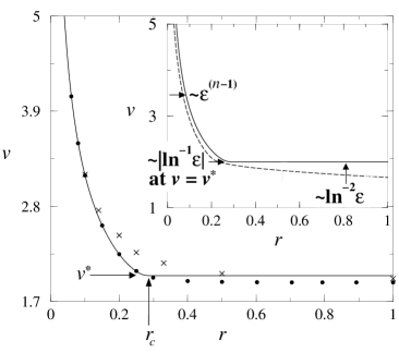
Figure 2: Comparison of simulation data for $v_{\text{as}}(\varepsilon,r)$ with the analytical prediction (7), which is plotted as the solid line. The solid dots in Fig. 2 represent the numerical data for Eq. (3) with $\varepsilon=2\times 10^{-5}$ and $n=3$. The crosses are the data points for fronts in the stochastic growth model described in the text. Inset: illustration of the leading order rate of convergence of the $v_{\text{as}}(\varepsilon,r)$ curve to the $\varepsilon\rightarrow 0$ limit, by means of the schematic dashed curve.

Figure 3: Numerical data for $v_{\text{as}}(\varepsilon,r)$ as a function of $\varepsilon$ for $n=2$ and $3$, at $r=0.2$. The graph demonstrates the insensitivity of $v$ to $\varepsilon$ for small values of $\varepsilon$ (note the fine scale on the vertical axis), as well as the convergence as $\varepsilon^{n-1}$ to its $\varepsilon\rightarrow 0$ value $\simeq 2.246$, given by Eq. (7), for two different values of $n$.

These expressions show that the limits do not commute for $r<r_{c}$: taking the limit $\varepsilon\to 0$ first in $f$ yields a front speed $v^{*}$ but the limit $v_{\text{as}}(\varepsilon\to 0,r)>v^{*}$. The reason is that for $r<r_{c}$ there is always a little tail of the front that runs faster than $v^{*}$ and makes $\phi$ nonzero. Once $\phi$ is nonzero, growth continues and the region behind it just has to follow it with the same asymptotic speed.

Our analysis is corroborated by numerical results obtained by solving Eq. (1) forward in time, (with Gaussian initial conditions). The data for $v$ vs. $r$ at $\varepsilon=2\times 10^{-5}$ are shown as solid dots in Fig. 2. Note that for $r<r_{c}$, the solid dots fall on top of our prediction (7) drawn with a solid line, while for $r>r_{c}$, they systematically fall below the solid line $v=v^{*}$. The reason for it is the difference between the rates of convergence as $\varepsilon\rightarrow 0$, which is illustrated in the inset of Fig. 2 by means of the schematically drawn dashed line. The arrows in the inset indicate the rate of convergence of the dashed $r$-$v$ curve towards the limiting one, given by Eq. (7). For $r>r_{c}$, the convergence is $\sim\ln^{-2}\varepsilon$ like in the case for $r=1$, analyzed in Ref. bd ; but for $r<r_{c}$ the convergence is much faster, $\varepsilon^{n-1}$. This latter behavior is illustrated for $r=0.2$ and $n=2,3$ in Fig. 3 — note the fine scale on the vertical axis!

That the effect of increasing asymptotic speed with decreasing $r$ below $r_{c}$ is a real effect for stochastic fronts too is illustrated by the crosses in Fig. 2: these represent the data for the average speed of fronts in a reaction-diffusion system X$\leftrightharpoons 2$X, for discrete X particles on a lattice with $N=10^{4}$ correspond , where the growth rates have been modified when the number of particles $n_{i}$ on a lattice site $i$ is less than $1/r$. In accord with the shape of the growth function $f$ illustrated in Fig. 1b, the rate at which particles are created at a lattice site $i$ with $1\leq n_{i}<1/r$ particles is simply taken to be the same as the rate for $n_{i}=1/r$ (corresponding to the integral values $1/r=1,2,3,4,5,7$ and $10$, due to the discreteness of particles). As one can see from Fig. 2, already when $r=0.5$, i.e., when only the growth rate at lattice sites with one particle is increased by a factor 2, the asymptotic growth speed is above the value $v^{*}=2$.

In the remainder of this paper, we derive the analytical results for the nonlinear diffusion equation with the growth function (3). Our analysis is based on the following observation: for $\varepsilon=0$, it is well known that the nonlinear diffusion equation allows a continuous family of front solutions with $v\geq v^{*}$. When such fronts solutions are parametrized by their velocity $v$, and when the growth rate is modified to allow a transition to a “pushed” front with velocity $v^{\dagger}$, it is also known vs2 ; ebert that solutions with $v<v^{\dagger}$ are unstable to a localized mode. In our analysis, we therefore consider a front with a given fixed velocity $v$ and, for small $\varepsilon$, determine when upon decreasing $r$ a localized mode of the stability operator crosses the eigenvalue zero. In the limit $\varepsilon\to 0$ this marks the selected pushed front in the $r$-$v$ diagram.

To carry out the linear stability analysis of the front solution, it is convenient to follow the standard route of transforming the linear eigenvalue equation into a Schrödinger eigenvalue problem bj ; ebert . We consider a function $\phi(x,t)$, which is infinitesimally different from the asymptotic front solution $\phi_{\text{as}}(\xi)$ in the comoving frame $\xi=x-vt$, i.e., $\phi(x,t)=\phi_{\text{as}}(\xi)+\eta(\xi,t)$. Upon linearizing Eq. (1) in the comoving frame, one finds that the function $\eta(\xi,t)$ obeys the following equation:

$$\frac{\partial\eta}{\partial t}\,=\,v\,\frac{\partial\eta}{\partial\xi}\,+\,\frac{\partial^{2}\eta}{\partial\xi^{2}}\,+\,\frac{\delta f(\phi)}{\delta\phi}\bigg{|}_{\phi\,=\,\phi_{\text{as}}}\,\eta\,.$$ (8)

Since this equation is linear in $\eta$, the question of stability can be answered by studying the spectrum of the temporal eigenvalues. To this end, we express $\eta(\xi,t)$ as

$$\eta(\xi,t)\,=\,e^{-\,Et}\,e^{-\,v\xi/2}\,\psi_{E}(\xi)\,,$$ (9)

which converts Eq. (8) to a one-dimensional Schrödinger equation for a particle in a potential with $\hbar^{2}/2m=1$:

$$\left[\,-\,\frac{d^{2}}{d\xi^{2}}+\frac{v^{2}}{4}-\frac{\delta f(\phi)}{\delta\phi}\bigg{|}_{\phi\,=\,\phi_{\text{as}}}\right]\psi_{E}(\xi)=\,E\,\psi_{E}(\xi),$$ (10)

In Eq. (10), the quantity $\displaystyle{V(\xi)=\left[\,\frac{v^{2}}{4}\,-\,\frac{\delta f(\phi)}{\delta\phi}\bigg{|}_{\phi\,=\,\phi_{\text{as}}}\right]}$ plays the role of the potential. It is easily obtained explicitly from the expression (3) for $f(\phi,\varepsilon,r)$ as

$$V(\xi) = \left[\,\frac{v^{2}}{4}-1+n\phi_{\text{as}}^{n-1}(\xi)\right]\Theta(\xi_{1}-\xi)$$ (11)

$$~{}~{}~{}~{}+\frac{v^{2}}{4}\,\Theta(\xi-\xi_{1})-\frac{1}{rv}\,\delta(\xi-\xi_{0})\,,$$

where $\phi(\xi_{0})=\varepsilon$ and $\phi(\xi_{1})=\varepsilon/r$. The form of the potential for $v>v^{*}$ and small $\varepsilon$ is sketched in Fig. 4. Keep in mind that $\phi_{\text{as}}(\xi)$ is a monotonically increasing function from $\varepsilon/r$ at $\xi_{1}$ towards the left, and that $\phi_{\text{as}}(\xi\to-\infty)=1$. As a result, in Fig. 4, $V(\xi)$ also increases monotonically towards the left for $\xi<\xi_{1}$. On the right of $\xi_{1}$, $V(\xi)$ is constant at $v^{2}/4$, and at $\xi_{0}$, there is an attractive $\delta$-function potential of strength $(rv)^{-1}$ notedelta . The crucial feature for the stability analysis below is the fact that $V(\xi)$ stays remarkably flat at a value $2\varepsilon/r$ over a distance $(\xi_{1}-\xi_{2})\simeq|\ln\varepsilon/r|$ deb2 , and on the left of $\xi_{2}$, it increases to the value of $v^{2}/4+n-1$, over a distance of order unity.

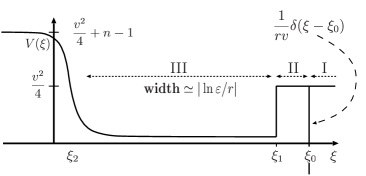
Figure 4: The potential $V(\xi)$ for $v\geq v^{*}$ and infinitesimally small $\varepsilon$ in the Schrödinger operator that determines the temporal eigenvalues of the stability analysis. $\xi_{2}$ marks the position of the region of finite width where the potential crosses over from the asymptotic value on the left where $\phi_{\text{as}}\approx 1$ to the value in the well where $\phi_{\text{as}}\ll 1$, $\xi_{1}$ the position of the step and $\xi_{0}$ the position of the delta function term in the potential.

If there exist negative eigenvalues of the Schrödinger equation (10), then according to Eq. (9), $\eta(\xi,t)$ grows in time in the comoving frame, i.e., the front solution $\phi_{\text{as}}(\xi)$ is unstable. For our purpose, therefore, we look for the value of $r$ at which there is a bound state of Eq. (10) with eigenvalue $E$, such that $E\rightarrow 0-$ for the potential sketched in Fig. 4. This is a problem in elementary quantum mechanics. For $\varepsilon\rightarrow 0$, the potential $V(\xi)$ is essentially constant in the left neighbourhood of $\xi_{1}$, and hence for $v>v^{*}$ and $E\rightarrow 0-$, $\psi_{E}(\xi)$ can be written as

$$\psi_{E}(\xi)\, = \,A_{-}e^{\lambda_{1}(\xi-\xi_{1})}\quad\quad\quad\quad\quad\quad~{}\mbox{for}\,\,\xi\leq\xi_{1}$$ (12)

$$= \,A\,e^{\lambda_{2}(\xi-\xi_{0})}+B\,e^{\lambda_{2}(\xi_{0}-\xi)}\quad\mbox{for}\,\,\xi_{1}\leq\xi\leq\xi_{0}$$

$$= \,A_{2}\,e^{-\lambda_{2}(\xi-\xi_{0})}\quad\quad\quad\quad\!\quad\quad\mbox{for}\,\,\xi>\xi_{0}\,,$$

where $\lambda_{1}=\sqrt{v^{2}/4-1}$ and $\lambda_{2}=v/2$. The function $\psi_{E}(\xi)$ must be continuous at $\xi_{1}$ and $\xi_{0}$, while its slope is continuous at $\xi_{1}$, but not at $\xi_{0}$. Matching of these boundary conditions to determine the value of $r$, where the bound state eigenvalue $E$ crosses zero, also requires an expression for the distance $\xi_{0}-\xi_{1}$. To this end, we divide the range of $\phi$ values between $0$ and $1$ into the three regions marked in Fig. 4: (i) region I, where $\phi_{\text{as}}<\varepsilon$, (ii) region II, where $\varepsilon\leq\phi_{\text{as}}<\varepsilon/r$, and (iii) region III, where $\phi_{\text{as}}\geq\varepsilon/r$. In the comoving frame, the asymptotic shape $\phi_{\text{as}}(\xi)$ of the front is the solution of the differential equation $\phi^{\prime\prime}_{\text{as}}\,+\,v\,\phi^{\prime}_{\text{as}}\,+\,f(\phi_{\text{as}},\varepsilon,r)\,=\,0\,$, where a prime denotes a derivative with respect to $\xi$. The solutions of $\phi_{\text{as}}(\xi)$ in the regions I and II that satisfy the continuity of $\phi_{\text{as}}(\xi)$ and $\phi_{\text{as}}^{\prime}(\xi)$, are respectively given by

$$\phi_{\text{as}}(\xi)\,=\,\varepsilon\,e^{-\,v(\xi\,-\,\xi_{0})}\quad\quad\quad\mbox{and}$$ (13)

$$\phi_{\text{as}}(\xi)=\left[\varepsilon-\frac{\varepsilon}{rv^{2}}\right]e^{v(\xi_{0}-\xi)}+\frac{\varepsilon\,(\xi_{0}-\xi)}{rv}+\frac{\varepsilon}{rv^{2}}.$$

The length $\xi_{0}-\xi_{1}$ of region II is obtained by equating $\phi_{\text{as}}(\xi_{1})$ from the second line of Eq. (13) to $\varepsilon/r$. After dividing out a factor of $\varepsilon/r$, this condition becomes

$$\left[\,r\,-\,\frac{1}{v^{2}}\right]\,e^{v(\xi_{0}-\xi_{1})}+\,\frac{\xi_{0}-\xi_{1}}{v}\,+\,\frac{1}{v^{2}}\,=\,1\,.$$ (14)

Thereafter, using Eqs. (12) and (13), one arrives at Eq. (7).

The above analysis yields the relation between $v$ and the critical value of $r$ in the limit $\varepsilon\to 0$. The convergence with $\varepsilon$, i.e., the rate of approach with $\varepsilon$ of the dashed curve to the solid one in Fig. 2, can be obtained by considering the effect of the $n\phi_{\text{as}}^{n-1}(\xi)$ term of $V(\xi)$ on the eigenfunctions and eigenvalues. For $v>v^{*}$, this term is simply a correction of order $\varepsilon^{n-1}$ to the finite bottom value of the potential. This term can be included perturbatively, and accordingly it leads to a shift of order $\varepsilon^{n-1}$ in the critical value of $r$. As Fig. 3 illustrates, this prediction is confirmed numerically. The case $v=v^{*}$ calls for a more detailed analysis, since the bottom value of the potential vanishes in the limit $\varepsilon\to 0$. In this case, it is known ebert ; bd that $\phi_{\text{as}}(\xi)\sim(C\xi+D)e^{-\xi}$, so $V(\xi)\simeq n(\varepsilon/r)^{n-1}(\xi/\xi_{1})^{n-1}e^{(n-1)(\xi_{1}-\xi_{)}}$ in the leading order of $\varepsilon$. In dominant order, we need to keep only the exponential behaviour, and the solution of $\psi_{E}(\xi)$ is then given by the Bessel function $A_{-}K_{0}(2\sqrt{n\varepsilon^{n-1}e^{-(n-1)(\xi_{1}-\xi)}/r^{n-1}}\,)$ in the left neighbourhood of $\xi_{1}$. The $|\ln^{-1}\varepsilon|$ scaling for the asymptotic approach of the dashed curve to the solid one is then easily obtained once the boundary conditions at $\xi_{1}$ and $\xi_{0}$ are matched with the use of Eq. (14).

The logarithmic convergence of $v$ to $v^{*}$ from below for $r>r_{c}$ can be understood from an argument along the lines of that for $r=1$ bd . For $v<v^{*}$, the front profile $\phi_{\text{as}}(\xi)$ in region III is of the form $\phi_{\text{as}}(\xi)\sim C\sin[k(\xi-\xi_{2})+\beta]e^{-\xi}$. For $r=1$, region II is absent; in that case, the matching to the profile in region I and the divergence of the width $\xi_{0}-\xi_{2}\simeq|\ln\varepsilon|$ implies $k\simeq\pi|\ln\varepsilon|^{-1}$. For $r_{c}<r<1$, the matching to region II will change the prefactor, but $k$ will still scale as $|\ln\varepsilon|^{-1}$ because the width of region III still diverges logarithmically. As for $r_{c}\leq r<1$, this translates into a scaling of $v^{*}-v$ as $|\ln\varepsilon|^{-2}$, with a prefactor that depends on $r$. Note that this scaling is nicely consistent with the convergence of the $r$-$v$ curve towards the point $(r_{c},v^{*})$ from the left, due to the fact that the slope of this curve vanishes at this point, and the convergence from below to this point scales as the square of the convergence from the left.

We finally end this paper with the note that if the (nonnegative) growth rate is bounded from above by $f(\phi,\varepsilon)$ in the interval $\phi\leq\varepsilon/r$, but is equal to $f(\phi,\varepsilon)$ for $\phi>\varepsilon/r$, then as $\varepsilon\rightarrow 0$, the asymptotic front speed converges to $v^{*}$ with the same logarithmic convergence of Eq. (2) for any $r$. It simply follows from the inequality $v_{\text{as}}(\varepsilon/r)<v<v_{\text{as}}(\varepsilon)$, where $v_{\text{as}}(\varepsilon)$ is given by Eq. (2).

D. P. wishes to acknowledge financial support from “Fundamenteel Onderzoek der Materie” (FOM).

References

(1) E. Ben-Jacob, H. R. Brand, G. Dee, L. Kramer, and
J. S. Langer, Physica D 14, 348 (1985).
(2) W. van Saarloos, Phys. Rev. A 39, 6367 (1989).
(3) U. Ebert and W. van Saarloos, Physica D 146, 1
(2000).
(4) E. Brunet and B. Derrida, Phys. Rev. E 56, 2597
(1997).
(5) H. P. Breuer, W. Huber, and F. Petruccione, Physica D
73, 259 (1994).
(6) R. van Zon, H. van Beijeren, and Ch. Dellago,
Phys. Rev. Lett. 80, 2035 (1998).
(7) D. A. Kessler, Z. Ner, and L. M. Sander,
Phys. Rev. E. 58, 107 (1998).
(8) L. Pechenik and H. Levine, Phys. Rev. E 59,
3893 (1999).
(9) D. Panja and W. van Saarloos, cond-mat/0109528.
(10) D. Panja and W. van Saarloos, Phys. Rev. E 65,
057202 (2002).
(11) E. Brener, H. Levine, and Y. Tu,
Phys. Rev. Lett. 66, 1978 (1991).
(12) This corresponds to and
for the model considered in PvS .
(13) The -function in Eq. (11) appears
from the functional derivative of in , since there is a
discontinuity of magnitude in
at
. This discontinuity contributes an
amount equal to
to . As according
to Eq. (13), the prefactor .