AN ALGORITHM GENERATING SCALE FREE GRAPHS

Abstract

We propose a simple random process inducing various types of random graphs and the scale free random graphs among others. The model is of a threshold nature and differs from the preferential attachment approach discussed in the literature before.

The degree statistics of a random graph in our model is governed by the control parameter $\eta$ stirring the pure exponential statistics for the degree distribution (at $\eta=0,$ when a threshold is changed each time a new edge added to the graph) to a power law (at $\eta=1$, when the threshold is frozen). The exponent $\gamma$ characterizing the power law can vary in the wide range $\gamma\in(1,\infty)$ and can be tuned in different values $\gamma_{\mathrm{in}}$ and $\gamma_{\mathrm{out}}$ for in-degrees and out-degrees probability distributions independently. For the intermediate values of $\eta$, the decay rate is mixed.

Taking different statistics for the threshold changes, one obtains dissimilar asymptotic profiles for the degree distribution having, in general, nothing to do with power laws at $\eta=1$, but still uniformly exponential at $\eta=0.$

PACS codes: 02.50, 05.40-a, 89.75.-k

1 Introduction

A wide variety of systems in biology, communication technology, sociology and economics are best described as complex networks of agents linked by various physical and informational links. Clearly, the architecture of such networks is crucially important for the vitality and performance of these systems. It is generally recognized that a thorough investigation of possible mechanisms which determine the topology of complex ”real-world” networks is necessary for understanding their behavior. Numerous studies of the Internet [1]-[2] and World Wide Web (WWW) [3]-[5], the web of human sexual contacts [6] and movie actors collaboration networks [7]-[11], national power-grids [11] and phone-call networks [12]-[13], protein folding [8, 20] and cellular networks [21]-[24], etc. have revealed, among other facts, that the probability that a node of these networks has $k$ connections follows a power law

$$P(k)\propto k^{-\gamma}$$ (1)

over a large range of $k$, with an exponent $\gamma$ that ranges between 1 and 3 depending on the system [25]. Such networks are called scale-free [9]. Many other ”real-world” networks display an inherently uniform exponential topology that still deviates from a Poisson distribution expected for usual random graphs $\mathbb{G}(N,p)$.

Recently, a model generating a scale-free network has been suggested in [9]. It establishes a random graph process in which vertices are added to the graph one at a time and connected to a fixed number of earlier vertices, selected with probabilities proportional to their degrees. This preferential attachment assumption is based on the idea that a new site is more likely to link to existing sites which are ”popular” at time the site is added. Numerical simulations for the above process reported in [9, 26] show that after many iterations the proportion of vertices with degree $k$ indeed obeys the power law (1) with the exponent $\gamma=3.$ In [27], the power law statistics for $P(k)$ in this model has been proven analytically, and it has been justified that $\gamma=3$.

Probably, a complex network formed by the citation patterns of scientific publications where the nodes standing for published articles and a directed edge representing a reference to a previously published article exhibiting the power law with the exponent $\gamma=3$ [28], can be well fitted by the above process as discussed in [9, 26, 27]. However, in other ”real-world” networks having degree sequences matching a power law these exponents usually deviate from $3$. For example, $\gamma=2.3\pm 0.1$ for the movie actors collaboration network [7, 8], $\gamma=2.1$ for a graph of long distance telephone calls made during a single day [12, 13], etc. To fit these deviations, one assumes that the preferential attachment for a real network is nonlinear [14, 15], i.e. the probability that a node $i$ attaches to node $j$ can be characterized by some function $\Pi(k)$ also following a power law with some index $\alpha.$

The effect of nonlinear preferential attachment $\Pi(k)$ on the network dynamics and topology was studied in [16]. They demonstrated that the scale free network topology holds only if $\Pi(k)$ is asymptotically linear and is destroyed otherwise. This way the exponent of the degree distribution $P(k)$ can be tuned to any value between 2 and $\infty$ [25].

Nevertheless, the detailed studies of various ”real-world” networks still challenge to the preferential attachment approach [9]. Some ecological networks such as food webs quantifying the interactions between species [17], some networks in linguistics [19], a network representing an aggregation of the WWW domains [18], etc. exhibit a scale free topology characterized by the indices $1<\gamma<2$. Moreover, for some networks, the in-degree and out-degree probability distributions are dissimilar: the WWW-topology where the nodes are the webpages and the edges are the hyperlinks that point from one document to another meets the power laws with $\gamma_{\mathrm{in}}=2.1$ and $\gamma_{\mathrm{out}}=2.72$ [29], the distributions of the total number of sexual partners in a single year indicate the power law decay with $\gamma=2.54\pm 0.2$ for females and $\gamma=2.31\pm 0.2$ for males [6]. A recent study [30] extends the results on the citation patterns (incoming links) of scientific publications ($\gamma_{\mathrm{in}}=3$, [28]) to the outgoing degree distribution obtaining that it has an exponential tail (not a Poisson distribution). This challenge stimulates a search for the new models inducing graphs of the scale free topology.

A random procedure which we use to generate scale free graphs draws back to the ”toy” model for a system being at a threshold of stability reported in [31] and to various coherent-noise models [32]-[33] discussed in connection to the standard sandpile model [34] developed in self-organized criticality, where the statistics of avalanche sizes and durations also take a power law form. The random process in our model begins with no edges at time $0,$ at a chosen vertex $i,$ and adds new edges linked to $i$, one at a time; each new edge is selected at random, uniformly among all outgoing edges not already present. When at some time a performance of the system occasionally exceeds a threshold value, the system looses its stability, so that the process stops at the given vertex and then starts again at some other vertex lacks of outgoing edges. This way the out-degree distribution of the resulting graph equals to the distribution of residence times below the threshold which is closely related to the ergodic properties of the system and its complexity, [31].

Although it has no a definite relation to the preferential attachment principle [9], probably, both algorithms are similar: we also monitor a global state of the system (while inspecting its stability) and introduce an auxiliary function (which is, in some sense, analogous to $\Pi(k)$) to characterize the ergodic properties of the system. Nevertheless, the model we propose in the present paper has also a distinguishing feature: we allow for the threshold value to quench with a given probability $\eta$, so that a natural control parameter in our model is the relative frequency of threshold changes. Varying this frequency, one can control the statistics of switching events (when the system performance parameter passes the stability threshold) tuning it from the truly exponential decay distribution (when the threshold representing the environmental stress changes each time a new edge added to the graph) to a power law with some exponent $\gamma$ when the threshold is frozen.

Among clear advantages of the proposed algorithm, one can mention its flexibility (the possible value of index $\gamma$ varies in the wide range $(1,\infty),$ the in-degree and out-degree statistics can be tuned independently, the variation of frequency $\eta$ switches $P(k)$ from an exponential decay to a power law) as well as its relative simplicity for both analytical and numerical studies.

The paper is organized as follows. In Sec. 2, we describe the model we introduce. In Sec. 3, we investigate the degree statistics for the random graphs generated in accordance with the introduced random procedure. Section 6 is devoted to conclusions.

2 Motivation and description of the model

Probably, the most fascinating property of living systems is a surprising degree of tolerance against environmental interventions revealing the robustness of the underlying metabolic and genetic networks [14, 22, 23]. A typical question which is usually posed in the literature in concern to this feature is on the role of the network topology in the error tolerance (see [25] and references therein). However, in the present work, we bring an opposite question to a focus: what is the network topology (say, of the protein-protein interactions map) resulted from the very durable evolution process selecting from among species enjoying sufficiently good adaptivity? A principle of evolutionary selection of a common large-scale structure of biological networks put forward in [23] is closely related to this question.

The most of biological systems exhibiting a high degree of adaptivity can be referred as systems being close to a stability threshold, so that a slight modification of the environment would prompt a drastic change in the system performance increasing or reducing the stamina of biological spices. From the dynamical systems point of view, such a behavior can be interpreted as a forcing of bifurcation parameter through a bifurcation point triggering the system into a new state. In our study, we do not refer to any definite physical system displaying such a complex behavior. Instead, following [31], we use a ”toy” model, in which the bifurcation parameter (the current state of the system characterized by its net performance) and the bifurcation point (the threshold of stability characterizing a challenge of the environments) are considered as random independent variables. It is supposed that the system is subjected to a bifurcation, when its net performance takes on values above the threshold. It is also important that all network’s changes acquired in the previous stages of evolution of the graph are not discarded, when the system suffers a bifurcation, but still into effect for the forthcoming evolution.

We shall characterize the current performance of the whole system by the real number $x\in[0,1].$ Another real number $y\in[0,1]$ plays the role of the stability threshold. The network is supposed to be stable until $x<y$ and is condemned otherwise. We consider $x$ as a random variable distributed with respect to some given probability distribution function (pdf) $f(u):[0,1]\to\mathbb{R}^{+}$. In a deterministic version of the model, $f$ would be an ergodic invariant density function on the phase space which has an essential influence on the system dynamics close to the stability threshold value.

The value of threshold $y$ also fluctuates reflecting the changes of environments and is also treated as a random variable distributed over the interval $[0,1]$ with respect to some other pdf $g(u):[0,1]\to\mathbb{R}^{+}$. In general, $f$ and $g$ are two arbitrary positive integrable functions satisfying the normalization condition

$$\int^{1}_{0}du{\ }f(u)=\int^{1}_{0}du{\ }g(u)=1.$$ (2)

We define the random procedure on the fixed set of $N$ vertices describing the evolution of network as a random graph evolving in time. The process begins with no edges at time $0,$ at a chosen vertex $i$. Given a fixed real number $\eta\in[0,1]$, we define a discrete time random process in the following way. At time $t=0,$ the variable $x$ is chosen with respect to pdf $f$, and $y$ is chosen with pdf $g$. If $x<y$, we add an edge selected at random, uniformly among all edges outgoing from $i$, the process continues and goes to time $t=1$. At time $t\geq 1,$ one of the following events happens:

i) with probability $\eta$, the random variable $x$ is chosen with pdf $f$ but the threshold $y$ keeps the value it had at time $t-1$. Otherwise,

ii) with probability $1-\eta,$ the random variable $x$ is chosen with pdf $f,$ and the threshold $y$ is chosen with pdf $g$.

If $x\geq y,$ the process at the given vertex ends and then resumes at some other vertex chosen randomly from the vertices having no outgoing edges yet; if $x<y,$ the process continues at the same vertex and goes to time $t+1.$

Eventually, when at some time $T$ limiting the duration of the ”monotonous” evolution of the graph, the process moves to some other vertex, and $i$ has exactly $k=T$ outgoing edges.

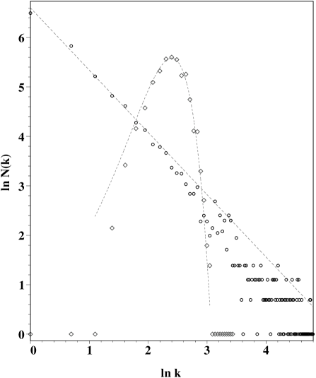
Figure 1: The proportion of vertices of degree $k$ versus $k$ in the log-log scale ($N=2000,$ ${\ }f=g=1,$ ${\ }\eta=1$). Out-degree statistics (circles) satisfies a power law, while the in-degree probability distribution is Gaussian with the most probable number of incoming links $k^{*}_{\mathrm{in}}=11.$

For example, in Fig. 1 we have presented the results of numerical simulation for the above algorithm for a network consisting of $2\times 10^{3}$ vertices, for $f=g=1$ and $\eta=1$. It displays the proportion of vertices having degree $k$ versus $k$ in the log-log scale. Circles stay for the out-degree $k_{\mathrm{out}}$ and diamonds are for the in-degree $k_{\mathrm{in}}.$ One can see that the out-degree probability distribution is fitted well by a power law, while the in-degree probability distribution forms a Gaussian profile centered at the most probable number of incoming links $k^{*}_{\mathrm{in}}=11.$

The same algorithm can be extended readily to moderate the incoming edges also. Let us consider three random variables $x,y,$ and $z$ that are the real numbers distributed in accordance to the distributions $f,$ $g$, and $v$ within the unit interval $[0,1].$ We assume that $x$ represents the current performance of the system, $y$ and $z$ are the thresholds for emission and absorption of edges respectively.

The generalized process begins on the set of $N$ vertices with no edges at time $0,$ at a chosen vertex $i$. Given two fixed numbers $\eta\in[0,1]$ and $\nu\in[0,1]$, the variable $x$ is chosen with respect to pdf $f$, $y$ is chosen with pdf $g$, and $z$ is chosen with pdf $v$, we draw $e_{ij}$ edge outgoing from $i$ vertex and entering $j$ vertex if $x<y$ and $x<z$ and continue the process to time $t=1.$ Otherwise, if $x\geq y$ ($x\geq z$), the process moves to other vertices having no outgoing (incoming) links yet.

At time $t\geq 1,$ one of the three events happens:

i) with probability $\eta$, the random variable $x$ is chosen with pdf $f$ but the thresholds $y$ and $z$ keep their values they had at time $t-1$.

ii) with probability $1-\eta,$ the random variable $x$ is chosen with pdf $f,$ and the thresholds $y$ and $z$ are chosen with pdf $g$ and $v$ respectively.

iii) with probability $\nu,$ the random variable $x$ is chosen with pdf $f$, and the threshold $z$ is chosen with pdf $v$ but the threshold $y$ keeps the value it had at time $t-1$.

If $x\geq y$, the process stops at $i$ vertex and then starts at some other vertex having no outgoing edges yet. If $x\geq z,$ the accepting vertex $j$ is blocked and does not admit any more incoming link (provided it has any). If $x<y$ and $x<z$, the process continues at the same vertex $i$ and goes to time $t+1.$

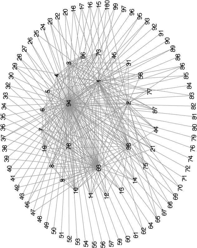
Figure 2: An example of a graph generated with the algorithm of Sec. 2 on the set of 100 vertices for the case of uniform densities $f=g=v=1,$ for $\eta=1.$

Figure 2 displays an example of a graph generated in accordance this algorithm on the set of 100 vertices for the case of uniform densities $f=g=v=1$ for $\eta=\nu=1.$ In Fig. 3, we have presented the distribution $P(k)$ vs. $k$ in the log-log scale over $10^{5}$ vertices. Here, the circles stay for outgoing degrees, and diamonds are for incoming degrees. For $k\gg 1,$ both profiles enjoy a power law decay with $\gamma_{\mathrm{in}}=\gamma_{\mathrm{out}}=2.$

In the forthcoming section, we demonstrate that for some probability densities $f,g$, and $v$ the resulting probability distribution $P(k)$ meets asymptotically a power law (1) as $k\gg 1$ where the index $\gamma$ can vary in the wide range $\gamma\in(1,\infty)$. Moreover, by means of adjusting probability densities $f,g,$ and $v$ from a proper class of functions, one can tune $\gamma_{\mathrm{in}}$ and $\gamma_{\mathrm{out}}$ to different values.

If $\nu=0$, both thresholds $y$ and $z$ have synchronized dynamics, and sliding the value of $\eta$ form 0 to 1, one can tune the statistics of out-degrees and in-degrees simultaneously out from the pure exponential decay to the power laws provided $f,$ $g$, and $v$ belong to the proper class of functions. When $\nu=1$, the threshold $z$ changes each time but the threshold $y$ is frozen. In this case, $P(k_{\mathrm{in}})$ decays exponentially for any choice of $v$, but $P(k_{\mathrm{out}})$ still meets a power law for $k_{\mathrm{out}}\gg 1$.

3 Probability degree distribution $P(k)$

Below, we compute the probability $P(k)$ that a given vertex has precisely $k$ outgoing edges as a result of the random procedure defined in the previous section. For sake of clarity, we investigate the statistics of switching events quenching the monotonous evolution of the graph in the simplest case when only one threshold ($y$) is present. All computations can be extended readily to the general case when both thresholds are present.

Directly from the definitions of Sec. 2, one can show that

$$P(0)=\int^{1}_{0}dy{\ }g(y)\int^{1}_{y}dx{\ }f(x).$$

In $t\geq 1$ time steps, the system can either ”survive” (S) or ”die” (D). Both issues can take place either in the ”correlated” way (with probability $\eta$, see i) (we denote these scenarios as $S_{c}$ and $D_{c}$ consequently), or in the ”uncorrelated” way (with probability $1-\eta$, see ii) ($S_{u}$ and $D_{u}$, consequently). For example, for $k=1$, we have

$$P(1)=P[SD_{c}]+P[SD_{u}]=\eta B(1)+(1-\eta)A^{2}(1)$$

where we have defined, for $n=0,1,2,\ldots,$

$$A(n)=\int_{0}^{1}dy{\ }g(y)\left[\int^{y}_{0}dx{\ }f(x)\right]^{n}$$ (3)

and

$$B(n)=\int_{0}^{1}dy{\ }g(y)\left[\int^{y}_{0}dx{\ }f(x)\right]^{n}\int^{1}_{y}du{\ }f(u)=A(n)-A(n+1).$$ (4)

Similarly,

$$P(2)=P[SS_{c}D_{c}]+P[SS_{c}D_{u}]+P[SS_{u}D_{c}]+P[SS_{u}D_{u}],$$

where

$$P[SS_{c}D_{c}]=\eta^{2}B(2),\quad P[SS_{c}D_{u}]=\eta(1-\eta)A(2)B(0),$$

$$P[SS_{u}D_{c}]=\eta(1-\eta)A(1)B(1),\quad P[SS_{u}D_{u}]=(1-\eta)^{2}A^{2}(1)B(0).$$

The general formula for $k\geq 3$ is tedious and can be found in [31].

Computations can be essentially simplified with the use of generating functions. Let us define the generating function for $P(k)$ by

$$\hat{P}(s)=\sum_{k=0}^{\infty}s^{k}P(k),\quad P(k)=\left.\frac{1}{k!}\frac{d^{k}\hat{P}(s)}{ds^{k}}\right|_{s=0},$$ (5)

and introduce the new auxiliary functions,

$$p(l)=\eta^{l}A(l+1),\quad\mathrm{for}{\ }l\geq 1,\quad p(0)=0,$$

$$q(l)=(1-\eta)^{l}A^{l-1}(1),\quad\mathrm{for}{\ }l\geq 1,\quad q(0)=0,$$

$$r(l)=\eta^{l}\left[\eta B(l+1)+(1-\eta)A(l+1)B(0)\right],\quad\mathrm{for}{\ }l\geq 1,\quad r(0)=0,$$

$$\rho=\eta B(1)+(1-\eta)A(1)B(0).$$ (6)

Then, the use of convolutions property [35] yields

$$\hat{P}(s)=B(0)+\rho s+\frac{s}{1-\hat{p}(s)\hat{q}(s)}\left[\hat{r}(s)+\rho\hat{p}(s)\hat{q}(s)+\rho A(1)\hat{q}(s)+A(1)\hat{q}(s)\hat{r}(s)\right],$$ (7)

where $\hat{p}(s),\hat{q}(s),\hat{r}(s)$ are the generating functions of $p(l),q(l),r(l),$ respectively.

In the marginal cases of $\eta=0$ and $\eta=1$, the probability $P(k)$ can be readily calculated.

3.1 The uncorrelated case, $\eta=0$

This case corresponds to the external stress being sensitive to any modification of a network and changing its figure as soon as a new edge appears in the graph. For $\eta=0,$ one has $\hat{p}(s)=\hat{r}(s)=0,$ and $\hat{q}(s)=s(1-sA(1))^{-1},$ ${\ }\rho=A(1)B(0)$, then equation (7) gives

$$\hat{P}_{\eta=0}(s)=\frac{B(0)}{1-sA(1)}.$$ (8)

Applying the inverse formula in (5) to equation (8), one arrives at

$$P_{\eta=0}(k)=A^{k}(1)B(0)=\left[\int^{1}_{0}dy{\ }g(y)\int^{y}_{0}dx{\ }f(x)\right]^{k}\int^{1}_{0}dy{\ }g(y)\int^{1}_{y}dx{\ }f(x).$$

Therefore, in the ”uncorrelated” case ($\eta=0$), for any choice of the pdf $f(u)$ and $g(u),$ the probability $P(k)$ decays exponentially.

3.2 The correlated case, $\eta=1$

Another marginal case corresponds to the external stress remaining unchanged during all time of network evolution. For $\eta=1$, one has $\hat{q}(s)=0,$ ${\ }\rho=B(1),$ and

$$s\hat{r}(s)=\sum^{\infty}_{n=1}s^{n+1}B(n+1)=\sum^{\infty}_{n=2}s^{n}B(n),$$

so that formula (7) yields

$$\hat{P}_{\eta=1}(s)=\hat{B}(s).$$ (9)

Consequently,

$$P_{\eta=1}(k)=B(k)=\int_{0}^{1}dy{\ }g(y)\left[\int_{0}^{y}dx{\ }f(x)\right]^{k}\int_{y}^{1}du\;f(u).$$ (10)

In the ”correlated” case, $\eta=1$, many different types of behaviour are possible, depending on the form of the pdf $f(u)$ and $g(u)$. We will examine an important class of $f(u)$ and $g(u)$, for which $P_{\eta=1}(k)$ can be explicitly computed from equation (10). We will take

$$\begin{array}[]{lc}f(u)=(1+\alpha)u^{\alpha},&\alpha>-1,\\ g(u)=(1+\beta)(1-u)^{\beta},&\beta>-1.\end{array}$$ (11)

Equation (10) gives in this case:

$$P_{\eta=1}(k)=\frac{\Gamma(2+\beta)\;\Gamma(1+k(1+\alpha))}{\Gamma(2+\beta+k(1+\alpha))}-\frac{\Gamma(2+\beta)\;\Gamma(1+(k+1)(1+\alpha))}{\Gamma(2+\beta+(k+1)(1+\alpha))}\;.$$

Using Stirling’s approximation, we get for large $k>>1$:

$$P_{\eta=1}(k)=\frac{(1+\beta)\;\Gamma(2+\beta)\;(1+\alpha)^{-1-\beta}}{k^{2+\beta}}\;\left(1+0\left(\frac{1}{k}\right)\right)\;.$$

For different values of $\beta$, the exponent of the threshold distribution, we get all possible power law decays of $P_{\eta=1}(k)$. Notice that the exponent $(-2-\beta)$ characterizing the decay of $P_{\eta=1}(k)$ is independent of the distribution $f(u)$ of the state variable.

Therefore, for $\eta=1$, one has to provide just one power law function (which defines the statistics of the threshold) to achieve a power law for $P(k)$ characterized by the exponent $\gamma\in(1,\infty).$

3.3 The case of uniform densities $f=g=1$

For the case of uniform densities $f=g=1,$ and after some tedious but trivial computation, we get from equation (7):

$$\hat{P}(s)=\frac{1}{1+(1-\eta)\mu(s)}\left[\frac{1+\mu(s)}{s}-\eta\mu(s)\right]\;,$$ (12)

where $\mu(s)$ is defined by

$$\mu(s)=\frac{\ln(1-\eta s)}{\eta s}\;.$$

The asymptotic behavior of $P(k)$ for $k$ large is determined by the singularity of the generating function $\hat{P}(s)$ that is closest to the origin.

For $\eta=0,$ the generating function has a simple pole $\hat{P}(s)=(2-s)^{-1},$ and therefore $P(k)$ decays exponentially, which agrees with the general conclusion of Sec. 3.1.

For intermediate values $1>\eta>0$, the generating function $\hat{P}(s)$ has two singularities. One pole, $s=s_{0},$ corresponds to the vanishing denominator $1+(1-\eta)\mu(s),$ where $s_{0}$ is the unique nontrivial solution of the equation

$$-\ln(1-\eta s)=s\frac{\eta}{1-\eta}\;.$$ (13)

Another singularity, $s=s_{1},$ corresponds to the vanishing argument of the logarithm, $s_{1}=\eta^{-1},$ such that $s_{1}>s_{0}>1.$ The dominant singularity of $\hat{P}(s)$ is of polar type, and the corresponding decay of $P(k)$ is asymptotically exponential for the degrees $k$ larger than $k_{c}\sim\ln(s_{0})^{-1}$, with a rate $\ln(s_{0})$ that vanishes like $1-\eta$ as $\eta$ tends to 1.

When $\eta$ tends to one, two singularities $s_{0}$ and $s_{1}$ merge. More precisely, we have

$$\hat{P}_{\eta=1}(s)=\frac{s+(1-s)\ln(1-s)}{s^{2}}.$$ (14)

The corresponding dominant term in (14) is of order $\mathrm{O}(k^{-2})$ [37]. This obviously agrees with the exact result one can get from equation (10), with $f(x)=g(x)=1$:

$$P_{\eta=1}(k)=\frac{1}{(k+1)(k+2)}\;.$$ (15)

In the case of uniform densities, it is possible to get an expression of $P(k)$ for all $k$, and for any value of $\eta$, by applying the inversion formula (5) to equation (14) and use of the formulae [36]. Combining all this, we get

$$P(k)=\frac{\eta^{k}}{(k+1)(k+2)}+\sum_{l=1}^{k}\frac{\eta^{k}}{(k-l+1)(k-l+2)\,l}\,\sum_{m=1}^{l}\left(\frac{1-\eta}{\eta}\right)^{m}c(m,l)\;,$$ (16)

where $c(m,l)$ is defined by

$$c(m,l)=m!\,\sum_{\begin{array}[]{c}\scriptstyle l_{1}+l_{2}+\cdots+l_{m}\,=\,l\\ \scriptstyle l_{i}\geq 1\end{array}}\hskip 284.52756pt$$

$$\frac{l_{1}\,l_{2}\,\cdots\,l_{m-1}\,l_{m}}{(l_{1}+1)\,(l-l_{1})\,(l_{2}+1)\,(l-l_{1}-l_{2})\,\cdots\,(l_{m-1}+1)\,(l-l_{1}-l_{2}-\cdots-l_{m-1})\,(l_{m}+1)}\;.$$

When $\eta\neq 0$, there is an alternative way of writing the previous expression:

$$P(k)=\frac{\eta^{k}}{(k+1)(k+2)}+\sum_{l=1}^{k}\frac{\eta^{k+1}}{(k-l+1)(k-l+2)}\,\sum_{m=1}^{\infty}(1-\eta)^{m}\,b(m,l)\;,$$ (18)

where $b(m,l)$ is defined by

$$b(m,l)=\sum_{\begin{array}[]{c}\scriptstyle i_{1}+i_{2}+\cdots+i_{l}\,=\,l\\ \scriptstyle i_{j}\geq 0\end{array}}\frac{1}{(i_{1}+1)\,(i_{2}+1)\,\cdots\,(i_{m-1}+1)\,(i_{m}+1)}\;.$$

In Fig. 4, we have plotted these asymptotes in the log-linear scale for the consequent values $\eta=0,$ ${\ }\eta=0.5$, ${\ }\eta=0.7$, ${\ }\eta=0.9$, ${\ }\eta=1$ (bottom to top) together with the curves representing analytical results (15-16).

Notice that for $\eta\neq 1$, we only plot distributions $P(k)$ up to relatively small degrees ($k=16$, $k=25$) correspondent to short quiescent times in the system, since these times are already bigger then the crossover value $k_{c}(\eta)\sim 1/\ln(s_{0})$ to the exponential decay $\exp{(-\,\ln(s_{0})\,k)}$ (where $s_{0}$ is defined by the Eq. (13)). For much longer times, very few survivals are observed, and the statistics gets bad. Of course, $k_{c}(\eta)$ grows as the parameter $\eta$ tends to 1, so that we have good statistics for larger $k$.

4 Discussion and Conclusion

In this paper, we have presented a simple random procedure inducing various types of random graphs and the scale free random graphs among others. The model we use essentially differs from the preferential attachment approach [9] discussed in the literature before. The proposed approach is simple and more flexible both for numerical simulations and analytical studies. The model draws back to the original ”toy” model for a system being at a threshold of stability [31].

In the proposed model, the degree statistics of a random graph depends from the value of the control parameter $\eta$ stirring the pure exponential statistics of degrees (at $\eta=0,$ when the threshold value is sensitive to each new edge risen in the graph) to a power law (at $\eta=1$, when the threshold value is frozen). The exponent characterizing the power law depends as $\gamma=2+\beta$ from the power law probability density distribution of the threshold $g(u)\propto(1-u)^{\beta},$ ${\ }\beta>-1,$ and can vary in the wide range $\gamma\in(1,\infty).$ For the intermediate values of $\eta$, the decay rate is mixed. In particular, we showed that, even if the asymptotic behavior is exponential, when $\eta$ is close to 1 this only holds for very large degrees $k$ of order of $(1-\eta)^{-1}$. The model can be readily generalized to various particular types of networks. The crucial advantage of the model is that, for most physically meaningful distributions, it can be solved analytically. In other cases, a numerical solution can be readily found.

In the present paper, we have limited the consideration to the special cases of uniform and power law distributions of thresholds. Indeed, one can take other (normalized) distributions for $f,g,$ and $v$ in this model and obtain different decaying asymptotic profiles for $P(k)$ either for synchronous $\nu=0$ or asynchronous $\nu=1$ dynamics of thresholds, they have, in general, nothing to do with power laws at $\eta=1$, but still uniformly exponential at $\eta=0.$

5 Acknowledgements

One of the authors (D.V.) benefits from a scholarship of the Alexander von Humboldt Foundation (Germany) that he gratefully acknowledges.

Figure 3: The distribution $P(k)$ vs. $k$ in the log-log scale generated on $10^{5}$ vertices, $f=g=v=1,$ ${\ }\eta=1$. Here, the circles stay for outgoing degrees and diamonds are for incoming degrees. Both profiles enjoy a power law decay with $\gamma=2.$

Figure 4: The distribution $P(k)$ in log-linear scale for different values of the parameter $\eta$, ${\ }\eta=0.,$ ${\ }\eta=0.5,$ ${\ }\eta=0.7,$ ${\ }\eta=0.9$ and $\eta=1.0$ (bottom to top). Straight lines corresponds to the pure exponential decay ($\sim 2^{-k}$) observed in the case $\eta=0$, the results obtained from (16) for the intermediate values of $\eta$, and to the result (15) for $\eta=1.0$ (bottom to top).

References

- [1] M. Faloutsos, P. Faloutsos, and C. Faloutsos, Proc. ACM SIGCOMM, Comput. Commun. Rev. 29, 251 (1999).
- [2] R. Govindan, H. Tangmunarunkit, Proc. IEEE Infocom 2000, Tel Aviv.
- [3] R. Albert, H. Jeong, A.-L. Barabási, Nature 401, 130 (1999).
- [4] J. M. Kleinberg, R. Kumar, P. Raghavan, S. Rajagopalan, A. Tomkins, Proc. of the International Conference on Combinatorics and Computing (1999).
- [5] R. Kumar, P. Raghavan, S. Rajagopalan, A. Tomkins, Proc. of the 9-th ACM Symposium on Principles of Database Systems, 1 (1999).
- [6] F. Liljeros, C. R. Edling, L. A. N. Amaral, H. E. Stanley, Y. Aberg, Nature 411, 907 (2001).
- [7] R. Albert, H. Jeong, A.-L. Barabási, Nature 406, 378; Erratum (2001), Nature 409, 542 (2001).
- [8] L. A. N. Amaral, A. Scala, M. Barthélémy, H. E. Stanley, Proc. Nat. Acad. Sci. USA 97, 11149 (2000).
- [9] A.-L. Barabási, R. Albert, Science 286, 509 (1999).
- [10] M. E. J. Newman, S. H. Strogatz and D. J. Watts, arXiv:cond-mat/0007235 (2000).
- [11] D. J. Watts, S. H. Strogatz, Nature 393, 440 (1998).
- [12] J. Abello, P. M. Paradalos, M. G. C. Resende, DIMACS Series in Disc. Math. and Theor. Comp. Sci. 50, 119 (1999);
- [13] W. Aiello, F. Chung, L. Lu, in Proc. 32-nd ACM Symp. Theor. Comp. (2000).
- [14] H. Jeong, Z. Néda, A.-L. Barabási, arXiv:cond-mat/0104131 (2001).
- [15] M. E. J. Newman, arXiv:cond-mat/0104209 (2001).
- [16] P. L. Krapivsky, S. Render, F. Leyvraz, Phys. Rev. Lett. 85, 4629 (2000).
- [17] J. M. Montoya, R. V. Solé, arXiv:cond-mat/0011195 (2000).
- [18] L. A. Adamic, B. A. Huberman, Science 287, 2115 (2000).
- [19] R. Ferrer i Cancho, R. V. Solé, Santa Fe Preprint 01-03-016 (cited by [25]).
- [20] A. Scala, L. A. N. Amaral, M. Barthélémy, arZiv:cond-mat/0004380 (2000).
- [21] D. A. Fell, A. Wagner, Nature Biotechnology 18, 1121 (2000).
- [22] H. Jeong, B. Tombor, R. Albert, Z. N. Oltvai, A.-L. Barabási, Nature 407, 651 (2000).
- [23] H. Jeong, S. P. Mason, Z. N. Oltvai, A.-L. Barabási, Nature 411, 41 (2001).
- [24] A. Wagner, D. Fell, Tech. Rep. 00-07-041, Santa Fe Institute (2000).
- [25] R. Albert, A.-L. Barabási, arXiv:cond-mat/0106096 (2001).
- [26] A.-L. Barabási, R. Albert, H. Jeong, Physica A 272, 173 (1999).
- [27] B. Bollobás, O. Riordan, J. Spencer, G. Tusnády, Random Struct. Alg. 18, 279 (2001).
- [28] S. Redner, Euro. Phys. Journ. B 4, 131 (1998).
- [29] A. Broder, R. Kumar, P. Raghavan, S. Rajagopalan, A. Tomkins, J. Weiner, Comput. Netw. 33, 309 (2000).
- [30] A. Vasquez, arXiv:cond-mat/0105031 (2001).
- [31] E. Floriani, R. Lima, D, Volchenkov: A Toy Model for a System as a Threshold of Stability, Proceeding N 2001/082 of the International Workshop The Science of Complexity: From Mathematics to Technology to a Sustainable World, Zentrum für Interdisciplinäre Forschung (ZIF), Universität Bielefeld (Germany) (01.10.2000-31.08.2001) (submitted to Chaos). The computation of is performed by E. Floriani.
- [32] M. E. J. Newman, K. Sneppen, Phys. Rev. E 54, 6226 (1996).
- [33] K. Sneppen, M. E. J. Newman, Physica D 110, 209 (1997).
- [34] P. Bak, C. Tang, K. Wiesenfeld, Phys. Rev. Lett. 59, 381 (1987).
- [35] We use the convolution property,
-
[36]
We use the following facts for the computations:
where the latter equation is valid for all . - [37] Flajolet and Sedgewick, Analytic Combinatorics (preliminary version), chapter 5 (1993): INRIA Res. Rep. n. 2026 (http://algo.inria.fr/flajolet/Publications/books.html).