Mesoscopic effects in superconductor-ferromagnet-superconductor junctions

Abstract

We show that at zero temperature the supercurrent through the superconductor - ferromagnetic metal - superconductor junctions does not decay exponentially with the thickness $L$ of the junction. At large $L$ it has a random sample-specific sign which can change with a change in temperature. In the case of mesoscopic junctions the phase of the order parameter in the ground state is a random sample-specific quantity. In the case of junctions of large area the ground state phase difference is $\pm\pi/2$.

This work has been motivated by recent experiments [1, 2] on the superconductor-metallic ferromagnet-superconductor junctions where the ground state of the system with the superconducting phase difference equal to $\pi$ has been observed. It is well known that the sign of the critical supercurrent of pure SFS junctions oscillates with the width $L$ of the ferromagnetic region [3, 4, 5, 6]. This is due to the difference in Fermi momentum of electrons with different spins at the Fermi energy causing the superconducting wave function in the ferromagnetic region to oscillate with the characteristic distance $\hbar/(k_{\uparrow}-k_{\downarrow})$. Here $k_{\uparrow},k_{\downarrow}$ are Fermi momenta of up and down spins, which are different because of the finite exchange spin-splitting energy $I$ in ferromagnets.

It is important to note that in pure junctions the characteristic distance of oscillations is inversely proportional to $I$ and that at zero temperature the modulus of the critical current does not decay exponentially with $L$.

In the opposite limit of disordered ferromagnets $L\geq L_{I}=\sqrt{\frac{D}{I}}\geq l$ the average critical current $\langle I_{c}\rangle$ decays exponentially with $L$ and with temperature $T$ [1]

$$\langle I_{c}\rangle\sim Re\exp(-\frac{L}{\xi_{F}});\xi_{F}=\sqrt{\frac{\hbar D}{2(\pi T+iI)}}$$ (1)

(where brackets $\langle\rangle$ stand for averaging over the random realizations of the scattering potential and $D$ is the the electron diffusion coefficient in the ferromagnet. It is interesting however, that in addition to the exponential decay, the average critical current oscillates as a function of $L$. It also changes sign as a function of $T$, provided $D/L^{2}\stackrel{{\scriptstyle~{}}}{{<}}I$.

The value of $\langle I_{c}\rangle$ can be negative which means that in the ground state of the junction the phase difference $\phi$ of the superconducting order parameter is $\pi$ rather than zero. The experimentally measured critical current in this case is the absolute value $|I_{c}|$.

The oscillations of the average critical current have been observed experimentally [1, 2]. We would like to note, however, that according to Eq.1 , these oscillations can be observed only in the case when the exchange spin-splitting energy in the ferromagnet is relatively small so that the characteristic distance of oscillations is large. This limits significantly the choice of ferromagnetic metals which can be used in the junctions to observe this effect.

In this paper we show that the exponential decay of the supercurrent with $L$ in Eq.1 originates from the averaging procedure. Before averaging over the impurity configurations at $L\gg L_{I}$ the supercurrent $I_{s}(\phi,L)$ has a random sample-specific sign while its modulus does not decay exponentially. The practical consequence of this conclusion is that the Josephson effect survives in the case of ferromagnets with large $I$ when $L\gg L_{I}$. We would like to mention that this feature is a particular case of a general statement that the Friedel oscillations in disordered metals do not decay exponentially at zero temperature [7, 8].

Below we discuss the limit of thick SFS junctions $L\gg L_{I}$ when their superconducting properties are determined by mesoscopic effects. We show that in this case the critical current of the junctions does not depend on the spin splitting $I$. The ground state of such a junction is, generally speaking, doubly degenerate with the phase difference having a random sample-specific modulus distributed in the interval ($0,\pi$). We also show that the critical current undergoes random oscillations as a function of $T$. Thus the junctions with $L\gg L_{I}$ should exhibit the same sequence of effects as the junctions with $L<L_{I}$.

The energy of the Josephson junction $E(\phi)$ is an even and periodic function of the phase of the order parameter. It can be represented in the form

$$E(\phi)=\sum_{n=1}^{\infty}E_{n}\cos n\phi$$ (2)

while the current through the contact is determined by the relation $J=2e\frac{dE}{d\phi}$. The coefficients $E_{n}$ are random sample-specific quantities. For $L\gg L_{I}$ all average coefficients $\langle E_{n}\rangle\sim\exp(-L/L_{I})$ are exponentially small. In this case the typical values of the coefficients $E_{n}$ can be estimated from their variances. To simplify the analysis we consider the case when the superconductors and the ferromagnet are separated by tunneling barriers of small transparency. We will show below that at $D/L^{2}\geq T$ and $L\geq\xi$ we have

$$\langle(E_{1})^{2}\rangle=S\xi^{2}(\frac{g}{8\pi\nu_{0}D})^{4}(\frac{D}{2\pi^{2}L^{2}})^{2}$$ (3)

$$\langle(E_{2})^{2}\rangle=S\xi^{2}(\frac{g}{8\pi\nu_{0}D})^{8}\frac{1}{(4\pi)^{3}}\frac{\xi^{2}D^{2}}{L^{2}}$$ (4)

(where $S$ is the area of the junction, $\nu_{0}$ is the density of states per spin in the ferromagnet, $\xi$ is the zero-temperature coherence length in the superconductor and $g$ is the conductance per unit area of the surface between the ferromagnet and the superconductor. Eqs. 3,4 correspond to the diagrams shown in Figures 1.b),c). In the case when the tunneling transmission coefficient of the insulator between the superconductor and the ferromagnet is small, the typical amplitude $(\langle(E_{2})^{2}\rangle)^{1/2}$ of the second harmonic contains an additional power of $g$ compared to the amplitude $(\langle(E_{1})^{2}\rangle)^{1/2}$ of the first harmonic and therefore for typical samples of low $g$, $E(\phi)$ is well approximated by the first harmonic. Since $(\langle(E_{1})^{2}\rangle)^{1/2}$ does not decay exponentially with $L$, it is much larger than $\langle E_{1}\rangle$. This means that $E_{1}$ has a random sign. In the cases when $E_{1}<0$ the ground state of the junction corresponds to $\phi_{GS}=\pi$.

The correlation function $\langle E_{1}E_{2}\rangle$ contains an additional power of $g$ with respect to $\langle(E_{2})^{2}\rangle$ and can be neglected which means that $E_{1}$ and $E_{2}$ are random uncorrelated quantities. In rare samples where the amplitude of the first harmonic is small $(E_{1}\sim E_{2})$ one has to take into account the second harmonic in Eq.2. In this case the ground state is doubly degenerate and corresponds to the phase difference

$$\phi_{GS}\sim\pm\arccos\frac{E_{1}}{4E_{2}}$$ (5)

Therefore the sample-specific random absolute value of the ground state phase difference is in the interval $0<|\phi_{GS}|<\pi/2$, provided $|E_{1}|<4|E_{2}|$. The probability of such an event is of order

$$\sqrt{\frac{\langle(E_{2})^{2}\rangle}{\langle(E_{1})^{2}\rangle}}\sim\xi L(\frac{g}{8\pi\nu_{0}D})^{2}$$ (6)

We would like to mention that in the case of a transparent superconductor-ferromagnet boundary $\phi_{GS}$ is a random sample-specific quantity of order one.

Let us now discuss the temperature dependence of the critical current $I_{c}(T)$. To do so we calculate the correlation function

$$\langle E_{1}(T_{1})E_{1}(T_{2})\rangle\sim\exp(-2L\sqrt{\pi(T_{1}+T_{2})/D})$$ (7)

It follows from Eq.7 that the quantities $\langle(E_{1}(T))^{2}\rangle\sim\exp(-2^{3/2}L\sqrt{T/D})$ and $\langle(E_{1}(T)E_{1}(0)\rangle\sim\exp(-2L\sqrt{T/D})\rangle$ decay with different rates as $T$ increases. This indicates that in addition to an exponential decay, the quantity $E_{1}(T)$ exhibits random sample-specific oscillations with a period of order $T^{*}\sim D/L^{2}$.

The results presented above were obtained in the approximation when the variations of the phase of the order parameter along the superconductor-ferromagnet surface are neglected. This is a good approximation for the samples of small area. Below we show that in the samples of large area the possibility of spatial fluctuations of the order parameter phase along the superconductor- ferromagnet surface leads to an average critical current which is proportional to the area of the junction and does not decay exponentially even in the limit when $L\gg L_{I}$. In this case the ground state of the junction is doubly degenerate and

$$\phi_{GS}=\pm\pi/2$$ (8)

This can be shown using an expression for the effective Josephson energy

$$E=\int E_{c}({\mathchoice{{\hbox{\boldmath$\displaystyle\rho$}}}{{\hbox{\boldmath$\textstyle\rho$}}}{{\hbox{\boldmath$\scriptstyle\rho$}}}{{\hbox{\boldmath$\scriptscriptstyle\rho$}}}})\cos\phi({\mathchoice{{\hbox{\boldmath$\displaystyle\rho$}}}{{\hbox{\boldmath$\textstyle\rho$}}}{{\hbox{\boldmath$\scriptstyle\rho$}}}{{\hbox{\boldmath$\scriptscriptstyle\rho$}}}})d{\mathchoice{{\hbox{\boldmath$\displaystyle\rho$}}}{{\hbox{\boldmath$\textstyle\rho$}}}{{\hbox{\boldmath$\scriptstyle\rho$}}}{{\hbox{\boldmath$\scriptscriptstyle\rho$}}}}+\frac{N_{s}}{2m}\int d{\bf r}({\bf\nabla}\phi({\bf r})^{2})$$ (9)

where $\textstyle\rho$ is the coordinate along the surface between the superconductor and the ferromagnet, the ${\bf r}$-integration is performed in the bulk of the superconductors, $m$ is the electron mass, and $N_{s}$ is the superfluid density in superconductors. Eq.9 is valid on a scale larger than $L$ along the surface. The random function $E_{c}({\bf y})$ is characterized by its average $\langle E_{c}({\mathchoice{{\hbox{\boldmath$\displaystyle\rho$}}}{{\hbox{\boldmath$\textstyle\rho$}}}{{\hbox{\boldmath$\scriptstyle\rho$}}}{{\hbox{\boldmath$\scriptscriptstyle\rho$}}}})\rangle=0$ and a quickly decaying (at $|{\mathchoice{{\hbox{\boldmath$\displaystyle\rho$}}}{{\hbox{\boldmath$\textstyle\rho$}}}{{\hbox{\boldmath$\scriptstyle\rho$}}}{{\hbox{\boldmath$\scriptscriptstyle\rho$}}}}-{\mathchoice{{\hbox{\boldmath$\displaystyle\rho^{\prime}$}}}{{\hbox{\boldmath$\textstyle\rho^{\prime}$}}}{{\hbox{\boldmath$\scriptstyle\rho^{\prime}$}}}{{\hbox{\boldmath$\scriptscriptstyle\rho^{\prime}$}}}}|>L$) correlation function $\langle E_{c}({\mathchoice{{\hbox{\boldmath$\displaystyle\rho$}}}{{\hbox{\boldmath$\textstyle\rho$}}}{{\hbox{\boldmath$\scriptstyle\rho$}}}{{\hbox{\boldmath$\scriptscriptstyle\rho$}}}})E_{c}({\mathchoice{{\hbox{\boldmath$\displaystyle\rho^{\prime}$}}}{{\hbox{\boldmath$\textstyle\rho^{\prime}$}}}{{\hbox{\boldmath$\scriptstyle\rho^{\prime}$}}}{{\hbox{\boldmath$\scriptscriptstyle\rho^{\prime}$}}}})\rangle\simeq$ $\langle E_{c}({\mathchoice{{\hbox{\boldmath$\displaystyle\rho-\rho^{\prime}$}}}{{\hbox{\boldmath$\textstyle\rho-\rho^{\prime}$}}}{{\hbox{\boldmath$\scriptstyle\rho-\rho^{\prime}$}}}{{\hbox{\boldmath$\scriptscriptstyle\rho-\rho^{\prime}$}}}})E_{c}(0)\rangle\simeq\langle(E_{1}(S=L^{2}))^{2}\rangle/L^{4}$. The phase difference $\phi({\mathchoice{{\hbox{\boldmath$\displaystyle\rho$}}}{{\hbox{\boldmath$\textstyle\rho$}}}{{\hbox{\boldmath$\scriptstyle\rho$}}}{{\hbox{\boldmath$\scriptscriptstyle\rho$}}}})=\langle\phi\rangle+\delta\phi({\mathchoice{{\hbox{\boldmath$\displaystyle\rho$}}}{{\hbox{\boldmath$\textstyle\rho$}}}{{\hbox{\boldmath$\scriptstyle\rho$}}}{{\hbox{\boldmath$\scriptscriptstyle\rho$}}}})$ is a random function of $\textstyle\rho$. At small $E_{1}$ $\delta\phi({\mathchoice{{\hbox{\boldmath$\displaystyle\rho$}}}{{\hbox{\boldmath$\textstyle\rho$}}}{{\hbox{\boldmath$\scriptstyle\rho$}}}{{\hbox{\boldmath$\scriptscriptstyle\rho$}}}})\ll 1$. Minimizing Eq.9 with respect to $\delta\phi({\mathchoice{{\hbox{\boldmath$\displaystyle\rho$}}}{{\hbox{\boldmath$\textstyle\rho$}}}{{\hbox{\boldmath$\scriptstyle\rho$}}}{{\hbox{\boldmath$\scriptscriptstyle\rho$}}}})$ we get an expression for the effective energy per unit area [9]

$$E_{eff}=-E_{1}^{eff}\sin^{2}\langle\phi\rangle$$ (10)

(where $E_{1}^{eff}\simeq\frac{m}{N_{s}\xi L^{2}}\langle(E_{1}(S=L^{2}))^{2}\rangle$), determining the average critical current density as $\langle I_{c}\rangle=2eE_{1}^{eff}$ and the average phase difference in the ground state as given by Eq.8.

The results in Eqs.3,4 were calculated microscopically describing the SFS junction by a Hamiltonian of the form

$$\widehat{H}=\widehat{H}_{BCS}+\widehat{H}_{T}+\widehat{H}_{F}$$ (11)

where $\widehat{H}_{BCS}$ is the Hamiltonian of superconducting leads, the Hamiltonian

$$\widehat{H}_{T}=t\sum\limits_{i=1,2;\alpha}\int_{S_{i}}d{\mathchoice{{\hbox{\boldmath$\displaystyle\rho$}}}{{\hbox{\boldmath$\textstyle\rho$}}}{{\hbox{\boldmath$\scriptstyle\rho$}}}{{\hbox{\boldmath$\scriptscriptstyle\rho$}}}}_{i}\left(\Psi_{i}^{+}\left({\mathchoice{{\hbox{\boldmath$\displaystyle\rho$}}}{{\hbox{\boldmath$\textstyle\rho$}}}{{\hbox{\boldmath$\scriptstyle\rho$}}}{{\hbox{\boldmath$\scriptscriptstyle\rho$}}}}_{i},z_{i};\alpha\right)\Psi_{F}\left({\mathchoice{{\hbox{\boldmath$\displaystyle\rho$}}}{{\hbox{\boldmath$\textstyle\rho$}}}{{\hbox{\boldmath$\scriptstyle\rho$}}}{{\hbox{\boldmath$\scriptscriptstyle\rho$}}}}_{i},z_{i};\alpha\right)+h.c\right)$$ (12)

describes tunneling between superconductors labeled by $i=1,2$ and the ferromagnetic metal ($z_{1}=0,z_{2}=L$), labeled by index $F$, and $\alpha$ is the spin index. The integration is taken over the surfaces between superconductors and the ferromagnetic metal. The last term in Eq.11 corresponds to the disordered ferromagnetic metal unperturbed by the presence of superconductors, where spin up and down bands are split by the exchange field $I$

$$\widehat{H}_{F}=\widehat{H}_{0}+I\int d{\bf r}\Psi_{F}^{+}\left({\bf r};\alpha\right){\bf\sigma}_{\alpha\beta}^{z}\Psi_{F}\left({\bf r};\beta\right){\bf.}$$ (13)

Here $\widehat{H}_{0}$ is the Hamiltonian of noninteracting electrons which contains the operators of the kinetic energy and a random field $U\left({\bf r}\right)$ . We assume that the random potential is white-noise correlated so $\left\langle U\left({\bf r}\right)\right\rangle=0$ and $\left\langle U\left({\bf r}\right)U\left({\bf r}^{\prime}\right)\right\rangle=\left(2\pi\nu_{0}\tau\right)^{-1}\delta\left({\bf r}-{\bf r}^{\prime}\right)$ (where $\tau$ is the mean free time).

In the lowest order in tunneling through the superconductor-ferromagnet boundary we get

$$E_{1}=\frac{T}{2}\sum\limits_{\epsilon_{k};\alpha}t^{4}\int_{S_{1};S_{2}}d{\mathchoice{{\hbox{\boldmath$\displaystyle\rho$}}}{{\hbox{\boldmath$\textstyle\rho$}}}{{\hbox{\boldmath$\scriptstyle\rho$}}}{{\hbox{\boldmath$\scriptscriptstyle\rho$}}}}_{1}d{\mathchoice{{\hbox{\boldmath$\displaystyle\rho$}}}{{\hbox{\boldmath$\textstyle\rho$}}}{{\hbox{\boldmath$\scriptstyle\rho$}}}{{\hbox{\boldmath$\scriptscriptstyle\rho$}}}}_{2}d{\mathchoice{{\hbox{\boldmath$\displaystyle\rho$}}}{{\hbox{\boldmath$\textstyle\rho$}}}{{\hbox{\boldmath$\scriptstyle\rho$}}}{{\hbox{\boldmath$\scriptscriptstyle\rho$}}}}_{1}^{\prime}d{\mathchoice{{\hbox{\boldmath$\displaystyle\rho$}}}{{\hbox{\boldmath$\textstyle\rho$}}}{{\hbox{\boldmath$\scriptstyle\rho$}}}{{\hbox{\boldmath$\scriptscriptstyle\rho$}}}}_{2}^{\prime}\{F^{+}\left(\epsilon_{k};{\mathchoice{{\hbox{\boldmath$\displaystyle\rho$}}}{{\hbox{\boldmath$\textstyle\rho$}}}{{\hbox{\boldmath$\scriptstyle\rho$}}}{{\hbox{\boldmath$\scriptscriptstyle\rho$}}}}_{1},0;{\mathchoice{{\hbox{\boldmath$\displaystyle\rho$}}}{{\hbox{\boldmath$\textstyle\rho$}}}{{\hbox{\boldmath$\scriptstyle\rho$}}}{{\hbox{\boldmath$\scriptscriptstyle\rho$}}}}_{1}^{\prime},0\right)G_{-\alpha;-\alpha}\left(\epsilon_{k};{\mathchoice{{\hbox{\boldmath$\displaystyle\rho$}}}{{\hbox{\boldmath$\textstyle\rho$}}}{{\hbox{\boldmath$\scriptstyle\rho$}}}{{\hbox{\boldmath$\scriptscriptstyle\rho$}}}}_{1}^{\prime},0;{\mathchoice{{\hbox{\boldmath$\displaystyle\rho$}}}{{\hbox{\boldmath$\textstyle\rho$}}}{{\hbox{\boldmath$\scriptstyle\rho$}}}{{\hbox{\boldmath$\scriptscriptstyle\rho$}}}}_{2}^{\prime},L\right)F\left(\epsilon_{k};{\mathchoice{{\hbox{\boldmath$\displaystyle\rho$}}}{{\hbox{\boldmath$\textstyle\rho$}}}{{\hbox{\boldmath$\scriptstyle\rho$}}}{{\hbox{\boldmath$\scriptscriptstyle\rho$}}}}_{2}^{\prime},L;{\mathchoice{{\hbox{\boldmath$\displaystyle\rho$}}}{{\hbox{\boldmath$\textstyle\rho$}}}{{\hbox{\boldmath$\scriptstyle\rho$}}}{{\hbox{\boldmath$\scriptscriptstyle\rho$}}}}_{2},L\right)G_{\alpha;\alpha}\left(\epsilon_{k};{\mathchoice{{\hbox{\boldmath$\displaystyle\rho$}}}{{\hbox{\boldmath$\textstyle\rho$}}}{{\hbox{\boldmath$\scriptstyle\rho$}}}{{\hbox{\boldmath$\scriptscriptstyle\rho$}}}}_{2},L;{\mathchoice{{\hbox{\boldmath$\displaystyle\rho$}}}{{\hbox{\boldmath$\textstyle\rho$}}}{{\hbox{\boldmath$\scriptstyle\rho$}}}{{\hbox{\boldmath$\scriptscriptstyle\rho$}}}}_{1},0\right)+h.c\}$$ (14)

where $\epsilon_{k}=\pi(2k+1)T$ is the Matzubara frequency and $k=0,1,...$ is an integer. We use the usual diagrammatic technique for averaging the products of electron Green’s functions [10]. Diagrams for correlation functions $\left\langle\left(E_{1}\right)^{2}\right\rangle$ and $\left\langle\left(E_{2}\right)^{2}\right\rangle$ are shown in Fig.1.b),c). There are two important blocks in these diagrams. The first one corresponds to diffuson and cooperon ladder made of single particle Green’s functions in the ferromagnet. In the case of a large $I$ only diffusons and cooperons for parallel spins survive. They are equal to each other and the same as in the absence of the external magnetic field, satisfying the equation [11]

$$\left(-D{\bf\nabla}^{2}+\left|\epsilon_{k}-\epsilon_{k^{\prime}}\right|\right)C\left(\left|\epsilon_{k}-\epsilon_{k^{\prime}}\right|;{\bf r},{\bf r}^{\prime}\right)=\theta\left(-\epsilon_{k}\epsilon_{k^{\prime}}\right)\delta\left({\bf r}-{\bf r}^{\prime}\right)$$ (15)

We would also like to mention that for $I\tau\geq 1$ we can neglect contributions of diagrams shown in Fig.1.d).

The second block is the ladder made of the anomalous Green’s functions $F(\epsilon_{k};{\bf r},{\bf r}^{\prime})$ in the superconductor. This average can be expressed in terms of the averaged product of the advanced and retarded Green’s function in the normal metal. Since

$$F(\epsilon_{k};{\bf r},{\bf r}^{\prime})=-i\int\limits_{-\infty}^{\infty}{\displaystyle{dE\over 2\pi}}{\displaystyle{\Delta\over\Omega^{2}+E^{2}}}\left(G^{R}\left(E,{\bf r},{\bf r}^{\prime}\right)-G^{A}\left(E,{\bf r},{\bf r}^{\prime}\right)\right)$$ (16)

(where $\Omega^{2}\equiv\Delta^{2}+\epsilon_{k}^{2}$), the averaging $\left\langle F(\epsilon_{k};{\bf r},{\bf r}^{\prime})F(\epsilon_{k}^{\prime};{\bf r},{\bf r}^{\prime})\right\rangle$ is equivalent to the averaging of Green’s functions in the normal metal. The diffusion propagator $\left\langle F(\epsilon_{k};{\bf r},{\bf r}^{\prime})F(\epsilon_{k}^{\prime};{\bf r},{\bf r}^{\prime})\right\rangle\sim$ $P(\Omega,\Omega^{\prime};{\bf r},{\bf r}^{\prime})$ obeys the diffusion equation

$$\left(-D{\bf\nabla}^{2}+\Omega+\Omega^{\prime}\right)P(\Omega,\Omega^{\prime};{\bf r},{\bf r}^{\prime})={\displaystyle{1\over 2}}{\displaystyle{\Delta\over\Omega}}{\displaystyle{\Delta\over\Omega^{\prime}}}\delta\left({\bf r}-{\bf r}^{\prime}\right)$$ (17)

The result of integration of four electron Green’s functions over the surface in diagrams shown in Fig.1.b),c) is estimated as $\tau^{2}g$ , where $g$ is the dimensional tunneling conductance per unit area of the boundary.

The solution of Eq.15 satisfying the boundary conditions ${\displaystyle{d\over dz}}C\left(\left|\epsilon_{k}-\epsilon_{k^{\prime}}\right|;{\bf r},{\bf r}^{\prime}\right)=0$ at the superconductor - ferromagnet metal surfaces is given by ( for $z>z^{\prime}$ )

$$C\left(\left|\epsilon_{k}-\epsilon_{k^{\prime}}\right|;{\bf r},{\bf r}^{\prime}\right)=\theta\left(-\epsilon_{k}\epsilon_{k^{\prime}}\right)\int\frac{dq_{x}dq_{y}}{(2\pi)^{2}}\frac{\cosh(Q(z-L/2))\cosh(Q(z^{\prime}+L/2))}{DQ\sinh QL}e^{iq_{x}(x-x^{\prime})+iq_{y}(y-y^{\prime})}$$ (18)

where $Q=\sqrt{q^{2}+{\displaystyle{\left|\epsilon_{k}-\epsilon_{k^{\prime}}\right|\over D}}}$ . Substituting this expression into diagrams shown in Fig.1.b)c) we get

$$\left\langle\left(E_{1}\right)^{2}\right\rangle\sim S\xi^{2}(\frac{g}{8\pi\nu_{0}D})^{4}T^{2}\sum\limits_{\epsilon_{k};\epsilon_{k^{\prime}}}\theta\left(-\epsilon_{k}\epsilon_{k^{\prime}}\right)\int\frac{d^{2}{\bf q}}{(2\pi)^{2}}{\displaystyle{1\over\left(Q\sinh QL\right)^{2}}}$$ (19)

$$\left\langle\left(E_{2}\right)^{2}\right\rangle\sim S\xi^{4}D^{2}(\frac{g}{8\pi\nu_{0}D})^{8}T^{2}\sum\limits_{\epsilon_{k};\epsilon_{k^{\prime}}}\theta\left(-\epsilon_{k}\epsilon_{k^{\prime}}\right)\int{\displaystyle{d^{2}{\bf q}\over\left(2\pi\right)^{2}}}{\displaystyle{1\over\left(Q\sinh QL\right)^{4}}}$$ (20)

Calculating integrals in Eqs.19,20 we arrive at Eqs.3-4.

To calculate the temperature dependence $\left\langle E_{1}\left(T_{1}\right)E_{1}\left(T_{2}\right)\right\rangle$ we should substitute $\epsilon_{k}=\pi\left(2k+1\right)T_{1}$ and $\epsilon_{k^{\prime}}=\pi\left(2k+1\right)T_{2}$ into Eq.19 . Then for $L_{T_{1}}=(D/T_{1})^{1/2},L_{T_{2}}=(D/T_{1})^{1/2}<L$ we get $\left(\sinh QL\right)^{-2}=4\exp[-2L(q^{2}+(\pi T_{1}+\pi T_{2})/D)^{1/2}]$ and finally we arrive to Eq.7.

In conclusion we have shown that the critical current of a mesoscopic SFS junction at small temperatures does not decay exponentially with the ferromagnet thickness. It has a random sign, which changes with temperature. The ground state phase difference of the junction is a random quantity $0<\phi_{GS}<\pi/2$. In the case of junctions of large area the phase difference is $\phi_{GS}=\pi/2$. Let us estimate the typical value of the critical current using Eq.3. Taking, for example, iron as a ferromagnet with $L\sim\xi=3\times 10^{-6}$ cm, the area of the surface $S\sim 10^{-7}$ cm², the elastic mean free path $l\sim 10^{-6}$ cm and assuming that the transmission coefficient through the superconductor-ferromagnet boundary is of order one we get $I_{c}\sim 10^{-6}$ A. The estimate based on Eq.3 scales with the junction area as $\sqrt{S}$ and is valid at small $S$. For junctions of large area, Eq.10 implies that the critical current is proportional to $S$.

We express our thanks to M. Gershenzon, A.D.Kent and Z. Radović for valuable discussions.

This work was supported by Division of Material Sciences, U.S.National Science Foundation under Contract No. DMR-9205144 and (ZA) by Russian Fund for Fundamental Research 01-02-17794.

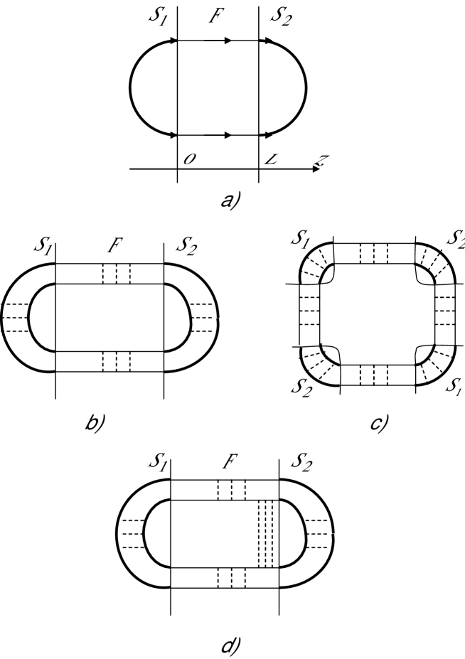
FIG. 1.: The diagrams contributing to: a) the current, to lowest order in transparency, b) the correlator $\langle E_{1}E_{1}\rangle,$ c) the correlator $\langle E_{2}E_{2}\rangle$, d) a diagram insignificantly contributing to the correlator $\langle E_{1}E_{1}\rangle$ in a superconductor - ferromagnet - superconductor junction. The symbols $S_{1}$ and $S_{2}$ correspond to the first and second superconductor respectively and $F$ denotes the ferromagnet. Thin lines represent the single electron Green’s functions, thick lines represent the anomalous Green’s functions, dashed lines denote averaging over the configurations of the impurity scattering potential. Ladders formed of Green’s functions and impurity scatterings in the ferromagnet correspond to diffuson or cooperon ladders.

REFERENCES

• [1] V.V.Ryazanov, V.A.Oboznov, A.Yu.Rusanov, A.V.Veretennikov, A.A.Golubov and J.Aarts, Phys.Rev.Lett. 86, 2427 (2001).
• [2] T.Kontos, M.Aprili, J.Lesueur, B.Stephanidis and R.Boursier, preprint cond-mat/0201104
• [3] A.I.Buzdin, L.N.Bulaevskii and S.V.Panyukov, JETP Lett. 35, 178 (1982) [Pis’ma Zh. Eksp. Teor. Fiz. 35, 147-148 (1982)
• [4] Z.RadoviΔ‡, L.DobrosavljeviΔ‡-GrujiΔ‡ and B.VujičiΔ‡, Phys.Rev.B 63, 214512 (2001).
• [5] F.S.Bergeret, A.F.Volkov and K.B.Efetov, Phys.Rev.B 64, 134506 (2001).
• [6] N.M.Chtchelkatchev, W.Beltzig, Yu.V.Nazarov, C.Bruder, JETP Lett., 74, 323, (2001).
• [7] B.Spivak, A.Zyuzin, JETP Lett. 47, 268, (1988).
• [8] B.Z.Spivak, A,Yu.Zyuzin, ”Mesoscopic fluctuations of current density in disordered conductors” in ” Mesoscopic phenomena in solids” ed. by B.L.Altshuler, P.A.Lee and R.A.Webb, Elsevier Science Publishers, Amsterdam 1991.
• [9] A.Zyuzin and B.Spivak, Phys.Rev.B 61, 5902 (2000).
• [10] A.A.Abrikosov, L.P.Gorkov, I.E.Dzyaloshinski, ”Methods of quantum field theory in statistical physics”, Dover Publications, New York 1963.
• [11] B.L.Altshuler, A.A.Aronov, in ”Electron-electron interactions in disordered systems”, ed.by A.L.Efros and M.Pollak, Elsevier Science Publishers, Amsterdam 1985.
Refer to caption