Magnetic moment of welded HTS samples:
dependence on the current flowing through the welds

Abstract

We present a method to calculate the magnetic moments of the high-temperature superconducting (HTS) samples which consist of a few welded HTS parts. The approach is generalized for the samples of various geometrical shapes and an arbitrary number of welds. The obtained relations between the sample moment and the density of critical current, which flows through the welds, allow to use the magnetization loops for a quantitative characterization of the weld quality in a wide range of temperatures and/or magnetic fields.

I Introduction

Practical applications of high-temperature superconductors (HTS) are based on the HTS ability to generate and to carry a current which produces magnetic field trying to compensate an external field Murakami . Thus, the HTS performance may be improved by increasing both the critical current density $j_{c}$ and the length scale $d$ over which a current flows Bean . An introduction of the melt-textured (MT) growth process MTG generally allowed to escape large-angle grain boundaries and to reach thereby quite suitable values of $j_{c}$ ($\approx 10^{5}\,A/cm^{2}$ at $T=77\,K$). So, over the last decade one spared no efforts to enlarge the sizes of HTS domains. Since a conventional growth of extra-large MT crystals ISTEC usually requires higher growth temperature (to avoid parasite-grain nucleation) and, hence, continues a very long time, various techniques to join separate HTS blocks were recently proposed Schatzle ; Philip ; Zheng98 ; Zheng99 ; Karapetrov ; Freyhardt ; Harnois ; Puig ; Bradley ; Noudem ; Prikhna . It stimulated a rapid development of experimental methods describing a quality of the superconducting joint, i.e. the density $j_{w}$ of critical current which may flow through it. Direct transport current measurements Philip ; Bradley ; Noudem , levitation force technique Zheng98 ; Zheng99 ; Kord , magneto-optical image analysis Zheng99 ; Puig and the Hall-probe magnetometry Philip ; Karapetrov ; Freyhardt ; Harnois ; Puig ; Prikhna were already used for these purposes.

Each of these methods has its merits and faults. Direct transport measurements, for example, are suitable only for relatively small and/or bad welds which critical current $I\sim j_{w}S$ still does not heat the sample because of the ohmic losses in the current pads. The common problems for the other, contactless techniques are their semi-quantitative nature and low functionality in strong magnetic fields. The scanning Hall-probe magnetometry, for example, to which these problems regard in the least degree, seems too sensitive to the test-bench geometry. Since the currents, which flow on different distances under the scanned sample surface, “smeared” a distribution of magnetic flux density above the weld, experimental data appear quite hard to interpret Matthias unless, certainly, the sample has the ideal geometric shape, i.e. flat, thin ring Zheng99 ; Karapetrov .

Meanwhile, both problems do not appear at all for the usual vibrating-sample magnetometry. The reason why it has so far mainly used for qualitative description of superconducting joints Philip ; Zheng99 and not gained a respectable reputation of an exact, quantitative method may be the following. Re-calculation of the critical current flowing through the weld(s) requires to know the magnetic moment of the sample divided onto parts/grains. In this work we present simple analytical equations for magnetic moments of split samples having some, most popular geometrical shapes. The approach is generalized for the case of $n$-slits and arbitrary sizes.

II Results and discussion

To generalize the estimation procedure for a quality $f=j_{w}/j_{m}$ of superconducting joints, where $j_{w}$ and $j_{m}$ are the densities of the critical current which may flow through a weld (intragrain current) and the original HTS material (intergrain current), let us first introduce the function $Q(f)=M(f)/M(f=1)$ which numerator and denominator are the magnetic moments of the welded samples with $j_{w}\neq j_{m}$ and $j_{w}=j_{m}$, respectively. One can readily predict that $Q$ generally depends on the sample geometry as well as on a quantity $n$ and a quality $f$ of superconducting joints. Having no aims to embrace the whole variety of shapes, we shall consider three common types presented in Figure 1, viz., the slabs split/welded along their short ($2a$) and long ($2b$) sides, which will hereafter be named $a$- and $b$-slabs, and the ring. By introducing the asymmetry factor

$$w=\left\{\begin{array}[]{ll}a/b,&\textrm{slabs}\\ (R_{2}-R_{1})/(R_{2}+R_{1}),&\textrm{ring}\\ \end{array}\right.$$ (3)

we intend to calculate the functions $Q(w,n,f)$ and to answer thereby the questions:

(Q1)

What geometry is the more sensitive to the current flowing through the joint(s)?

(Q2)

How to reconstruct its density $j_{w}$ proceeding from magnetic moment of the sample?

To obtain $Q(w,n,f)$ in simple analytical form which could be convenient for the experimental $j_{w}$ estimation, the following assumptions will be taken into account:

(A1)

the Bean’s critical state is valid, i.e. the currents penetrate all over the sample, their density everywhere equals to the critical current density of the HTS material which is independent of applied magnetic field $j_{m}(B)=Const$ and, finally, there is no flux creep.

(A2)

the joints are homogeneous over the whole joining surface, they have no width and separate the sample onto identical parts/grains;

(A3)

the welding process does not change the critical current density $j_{m}$ of the material itself.

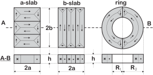
Figure 1: The sketch presents the sample geometries and schematic distribution of critical currents for the particular case of two slits, i.e. $n=2,\ f=0$. Depending on which side, either long $2b$ or short $2a$ one, appears parallel to the slits, the slabs are named $b$-slabs and $a$-slabs, respectively.

II.1 Search for the preferable geometry

Since the joints were accepted to have no width, no additional increase of magnetic moment should be expected when $j_{w}$ exceeds $j_{m}$ ($f\geq 1$). The functions $Q(w,n,f)$ must, therefore, cover the range between their minima, $Q(w,n,f=0)$, and unity. The more wide this range, the more sensitive appears a certain geometry to the current flowing through the joint(s). So, let us estimate the values of $Q(w,n,f=0)$ for chosen geometrical shapes.

Provided the assumptions (A1) are valid, the magnetic moment of homogeneous slab ($n=0$ or $f=1$) is presented Gyorgy ; Murakami by the simple equation

$$M(1)=V_{s}j_{m}a\left[1-w/3\right]/2,$$ (4)

where $V_{s}=2a\times 2b\times h$ is its volume and $w=a/b\leq 1$ is its asymmetry factor. Since $n$ slits ($j_{w}=0$) were presumed to split the original slab onto $N=n+1$ identical grains, the total moment of the split sample equals $N$ magnetic moments of each separate part. Thus, for $b$-slabs one can readily write

$$M(0) = V_{s}j_{m}a\left[1-w/(3N)\right]/(2N),$$ (5)

$$Q(0) = \frac{3N-w}{(3-w)N^{2}}.$$ (6)

Taking into account that numerous splitting of the $a$-slab may reverse long $2b/N$ and short $2a$ sides of its parts, one has to consider two cases

$$M(0) = V_{s}\frac{j_{m}}{2}\frac{b}{N}\left[1-\frac{1}{3wN}\right],\ wN\geq 1$$

$$M(0) = V_{s}\frac{j_{m}}{2}a\left[1-\frac{wN}{3}\right],\ wN\leq 1$$ (7)

which give

$$Q(0) = \frac{3wN-1}{(3-w)w^{2}N^{2}},\ wN\geq 1$$

$$Q(0) = \frac{3-wN}{3-w},\ wN\leq 1$$ (8)

Homogeneous ring ($n=0$ or $f=1$) may naturally be approximated by a superconducting turn which height, inner and outer radii are, respectively, $h$, $r_{i}$ and $r_{o}$. The turn cross-section $h(r_{o}-r_{i})$ allows to carry a current $I=j_{m}h(r_{o}-r_{i})$. The turn effective area $\bar{S}=\pi\bar{r}^{2}$ and its effective radius $\bar{r}$ are easy to obtain by standard averaging procedure of the function $S(r)=\pi r^{2}$ over the range $r_{i}\leq r\leq r_{o}$

$$\bar{S} = \left(\int_{r_{i}}^{r_{o}}S(r)dr\right)/(r_{i}-r_{o})=\frac{\pi}{3}\cdot\frac{r_{i}^{3}-r_{o}^{3}}{r_{i}-r_{o}},$$

$$\bar{r} = \sqrt{(r_{i}^{2}+r_{i}r_{o}+r_{o}^{2})/3}.$$ (9)

On substituting $r_{i}=R_{1}$ and $r_{o}=R_{2}$, the ring magnetic moment $M=I\bar{S}$ fits the equation

$$M(1)=\pi hj_{m}(R_{2}^{3}-R_{1}^{3})/3,$$ (10)

that appears from the well-known expression Brandt

$$M=\pi\int_{-h/2}^{+h/2}dz\int_{R_{1}}^{R_{2}}r^{2}\cdot j_{c}(r,z)dr,$$ (11)

describing any conductors which remain invariant to their rotation around the $z$-axis, e.g. toroids, disks, etc.

Similar approach may be applied to split rings or, at least, to those of them which are thin enough $w\ll 1$ and contain $n<\pi/(2w)$ slits. Figure 1 clearly shows that slits separate such rings onto two nearly full turns which carry the same circular currents $I=j_{m}h(R_{2}-R_{1})/2$, but flowing in opposite directions. Since non-circular currents on the left and right sides of each slit (the diamond-shaped areas in Figure 1) are antiparallel and, hence, nearly compensate each others, the magnetic moment of the split ring may be written as $M(0)=I(\bar{S_{1}}-\bar{S_{2}})[1-n\delta]$, where the small amendment $\delta\approx w/(2\pi)$ responds for reduction of the effective turn surfaces around each of $n$-slits. Substituting the inner and outer radii of the turns which are, respectively, equal to $R_{1}$ and $(R_{1}+R_{2})/2$ (for inner turn) and $(R_{2}+R_{1})/2$ and $R_{2}$ (for outer one) into Equations (9), one has

$$M(0) = \frac{1}{4}V_{r}j_{m}(R_{2}-R_{1})\left[1-\frac{wn}{2\pi}\right],$$ (12)

$$Q(0) = \frac{3}{4}\cdot\frac{k^{2}-1}{k^{2}+k+1}\left[1-\frac{wn}{2\pi}\right],$$ (13)

where the ring volume $V_{r}$ and its relative thickness $k$ are, respectively, $\pi(R_{2}^{2}-R_{1}^{2})h$ and $k=R_{2}/R_{1}=(1+w)/(1-w)$.

Split rings may also be approximated by replacing the radial arcs between the slits (see Figure 1) with slabs of the same sizes, viz., $(R_{2}-R_{1})$ and $\pi(R_{2}+R_{1})/n$. Then, by analogy with Equations (7) and (8), one writes

$$M(0) = \frac{\pi}{4n}V_{r}j_{m}(R_{2}+R_{1})\left[1-\frac{\pi}{3nw}\right],\ nw\geq\pi$$

$$M(0) = \frac{1}{4}V_{r}j_{m}(R_{2}-R_{1})\left[1-\frac{wn}{3\pi}\right],\ nw\leq\pi$$ (14)

$$Q(0) = \frac{3\pi}{4n}\cdot\frac{(k+1)^{2}}{k^{2}+k+1}\left[1-\frac{\pi}{3nw}\right],\ nw\geq\pi,$$

$$Q(0) = \frac{3}{4}\cdot\frac{k^{2}-1}{k^{2}+k+1}\left[1-\frac{wn}{3\pi}\right],\ nw\leq\pi.$$ (15)

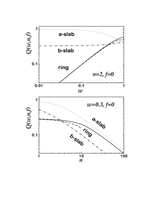
Figure 2: Typical dependencies of $Q(w,n,f=0)$ vs the asymmetry factor $w$ and vs the slit number $n$ confirm that better accuracy for the density $j_{w}$ of critical current flowing through the weld(s) will be ensured with the ring ($wn\ll 1$) and the $b$-slab ($wn\gg 1$) geometries of the sample. Double curve for the rings represent two approximations, viz. the “opposite turns” (solid line) and the “squared arcs” (dashed line) approximations given by the Equations (13) and (15), respectively.

Certainly, both the method of “opposite turns” (13) and that of “squared arcs” (15) give more accurate results for relatively thin rings $wn<1$. Fortunately, real rings usually satisfy this condition. Besides, the $Q(0)$ dependencies vs the sample asymmetry $w$ and these vs the slit number $n$ (see Figure 2) clearly indicate that within the range $wn>1$ definitely lower values of $Q(0)$ and, thus, better accuracy for the experimental $j_{w}$ calculation are provided by the $b$-slab geometry. Thus, further corrections for the rings with $wn\geq 1$ will scarcely have a practical value.

At last, one has to emphasize that the $a$-slabs ensure the worse accuracy. Moreover, their magnetic moments at $wn<0.1$ are almost independent of whether the intragrain current exists ($f>0$) or not ($f=0$).

II.2 Experimental method and its discussion

We have just obtained analytical solutions for the functions $Q(w,n,f)$ in the frontier points, $f=0$ and $f=1$. The range between them, $0<f<1$, may generally correction be represented by the linear combination

$$Q(f)=fQ(1)+(1-f)Q(0),$$ (16)

where the coefficient $(1-f)$ appears from an evident condition that the net (intergrain + intragrain) current can not exceed the critical current of the HTS material.

Thus, to estimate the target value of $j_{w}$, one has to know (i) magnetic moment of the welded sample, $M(f)$, as well as (ii) the critical current density $j_{m}$ of the HTS material. Within the suggestion (A3), it does not matter which experimental data, $M(1)$ or $M(0)$, are used to calculate $j_{m}$. Meantime, heating of MT HTS crystals up to the temperatures close to their peritectic points, what actually is the joining procedure Schatzle ; Philip ; Zheng98 ; Zheng99 ; Karapetrov ; Freyhardt ; Harnois ; Puig ; Bradley ; Noudem ; Prikhna , may sometimes lead to either reversible (e.g., the oxygen losses) or irreversible (e.g., the appearance of cracks and/or their expanding) changes in the HTS structure. If the latter yet happens, one may, as a last resort, propose to cut the welded sample again, to measure $M(0)$ and to recover both the genuine, “after-the-welding” value $j_{m}$ and the moment $M(1)$, in which this density could result, with aid of simple relations, (5)-(8) or (12)-(15). Finally, by substituting the obtained values, (i) $Q(f)=M(f)/M(1)$ and (ii) $j_{m}$, into equation

$$j_{w}=j_{m}\frac{Q(f)-Q(0)}{1-Q(0)},$$ (17)

we have the density of the current which flows through the weld(s). Respectively of the obtained quality, either $j_{w}<j_{m}$ or $j_{w}=j_{m}$, this current presents the critical current of the weld or of the HTS itself. The same remains valid for the other techniques and points out a vital necessity for experimenters to use a quantitative description, rather than to restrict themselves by qualitative comparison of superconducting welds with their unique HTS material. An ability of our method to discern the cases $j_{w}<j_{m}$ and $j_{w}=j_{m}$ and to give, at least, the lower estimate for the target value $j_{w}$ seems a worth compensation for twofold measurements of the magnetic moment.

There are other features, which favorably distinguish this approach, e.g., its good functionality in wide range of temperatures and magnetic fields, low requirements for the samples preparation as well as, generally speaking, the other advantages which de facto turned the magnetic moment measurements into the world-wide standard to study the superconducting properties.

References

- (1) Murakami M (Ed.) Melt-processed high-temperature superconductors, World Scientific, 1993
- (2) Bean C P 1964 Rev. Mod. Phys. 36 31
- (3) Jin S, Tiefel T H, Sherwood R C, Davis M E, van Dover R B, Kammlott G W, Fastnacht R and Keith H D 1988 Appl. Phys. Lett. 52 2074
- (4) Nagaya S 1997 ISTEC J. 10 31
- (5) Schätzle P, Krabbes G, Stoever G, Fuchs G and Schläfer D 1999 Supercond. Sci. Technol. 12 69
- (6) Vanderbemden Ph, Bradley A D, Doyle A D, Lo W, Astill D M, Cardwell D A and Campbell A M 1998 Physica C 302 257
- (7) Zheng H, Jiang M, Nikolova R, Vlasko-Vlasov V, Welp U, Veal B W, Crabtree G W, and Claus H 1998 Physica C 309 17
- (8) Zheng H, Jiang M, Nikolova R, Welp U, Paulikas A P, Huang Yi, Crabtree G W, Veal B W and Claus H 1999 Physica C 322 1
- (9) Karapetrov G, Cambel V, Kwok W K, Nikolova R, Crabtree G W, Zheng H and Veal B W 1999 J. Appl. Phys. 86 6282
- (10) Bradley A D, Doyle R A, Lo W, Cardwell D A and Campbell A M 1999 Supercond. Sci. Technol. 12 1054
- (11) Delamare M P, Walter H, Bringmann B, Leenders A and Freyhardt H C 2000 Physica C 329 160
- (12) Prikhna T, Gawalek W, Moshchil V, Surzhenko A, Kordyuk A, Litzkendorf D, Dub S, Melnikov V, Plyushchay A, Sergienko N, Koval’ A, Bokoch S and Habisreuther T 2001 Physica C 354 333
- (13) Harnois C, Desgardin C and Chaud X 2001 Supercond. Sci. Technol. 14 708
- (14) Puig T, Rodriguez P, Carrillo A E, Obradors X, Zheng H, Welp U, Chen L, Claus H, Veal B W and Crabtree G W 2001 Physica C 363 75
- (15) Noudem J G, Reddy E S, Tarka M, Noe M and Schmitz G J 2001 Supercond. Sci. Technol. 14 363
- (16) Kordyuk A A, Nemoshkalenko V V, Plyushchay A I, Prikhna T A and Gawalek W 2001 Supercond. Sci. Technol. 14 L41
- (17) Zeisberger M, et al. (to appear in Physica C )
- (18) Georgy E M, van Dover R B, Jackson K A, Schneemeyer L F and Warszczak J V 1989 Appl. Phys. Lett. 55 283
- (19) see, for example, Brandt E H, 2001 cond-mat/0104518 and references therein
- (20) Owing to nonlinear geometry of rings, linear approximation (16) is violated. However, a noticeable correction to the Equation (16) is required only for relatively thick rings, , at . For example, in the ring with , i.e. where the outer radius is twice larger than the inner one , the nonlinear amendment does not exceed 0.067