Low-temperature Metastability of Ising Models: Prefactors, Divergences, and Discontinuities

Abstract

The metastable lifetime of the square-lattice and simple-cubic-lattice kinetic Ising models are studied in the low-temperature limit. The simulations are performed using Monte Carlo with Absorbing Markov Chain algorithms to simulate extremely long low-temperature lifetimes. The question being addressed is at what temperatures the mathematically rigorous low-temperature results become valid. It is shown that the answer depends partly on how close the system is to fields at which the prefactor for the metastable decay either has a discontinuity or diverges.

1 Introduction

In many areas of science escape over a saddle point is an important physical phenomenon Book1 . In some cases results can be derived in the low-noise limit LowNoise . However, what is often missing is any idea of when the low-noise limit is applicable. This paper addresses the question of how low the noise must be before the metastable lifetime becomes dominated by the low-noise limit results.

Here the lifetime of the metastable state of the kinetic Ising model is studied. The square-lattice Ising model is studied using Glauber dynamics Glauber , as well as a dynamic derived from a coupling of a quantum spin $1\over 2$ system to a 1-dimensional phonon heat bath KParkCCP ; KParkUGA . The simple-cubic dynamic Ising model with a Glauber dynamic is also simulated in the low-temperature limit.

Although only specific cases are simulated, a reasonable hypothesis emerges as to the question of how low is a low enough temperature before the low-noise results are valid. The hypothesis is that it depends on how close the applied field is to a value where the low-temperature prefactor has a discontinuity or a divergence. As the field where the low-temperature prefactor has a discontinuity or divergence is approached, the low-temperature limit is seen at progressively lower temperatures.

2 Models and Methods

The Hamiltonian of a spin-$1\over 2$ system can be written as ${\mathcal{H}}={\mathcal{H}}_{\rm sp}+{\mathcal{H}}_{\rm bath}$. The spin Hamiltonian is

$${\mathcal{H}}_{\rm sp}=-J\sum_{\rm nn}\sigma_{i}^{z}\sigma_{j}^{z}-H_{z}\sum_{i}\sigma_{i}^{z}$$ (1)

where $J$ is the ferromagnetic ($J>0$) nearest-neighbor interaction parameter due to the exchange coupling between spins, $H$ is the applied external field, $\sigma^{z}_{j}$ is the $z$-component of the Pauli spin operator at site $j$, the first sum is over all nearest-neighbor (nn) pairs (4 nn for the square lattice and 6 for the simple-cubic lattice), and the second sum is over all $N$ spins.

To simulate the quantum system given by the Hamiltonian requires explicit knowledge of the heat bath to which the spin system is coupled. In general, simulating the complete quantum-mechanical system to obtain the time dependence of the spin degrees of freedom is unnecessary. With the given spin Hamiltonian, ${\mathcal{H}}_{\rm sp}$, the dynamic is determined by the generalized master equation KParkCCP ; KParkUGA ; BlumBook

$$\!\!\frac{{\mathrm{d}}\rho(t)_{m^{\prime}m}}{{\mathrm{d}}t} = \frac{i}{\hbar}[\rho(t),{\mathcal{H}}_{\mathrm{sp}}]_{m^{\prime}m}+\delta_{m^{\prime}m}\sum_{n\neq m}\rho(t)_{nn}W_{mn}-\gamma_{m^{\prime}m}\rho(t)_{m^{\prime}m}~{},$$ (2)

$$\gamma_{m^{\prime}m} = \frac{W_{m}+W_{m^{\prime}}}{2}\;,\;\;W_{m}=\sum_{k\neq m}W_{km}\;\;,$$ (3)

where $\rho(t)$ is the time dependent density matrix of the spin system, $m^{\prime}$, $n$, $k$, and $m$ denote the eigenstates of ${\mathcal{H}}_{\rm sp}$, $\rho(t)_{m^{\prime}m}$$=$$\langle m^{\prime}|\rho(t)|m\rangle$, and $W_{km}$ is a transition rate from the $m$-th to the $k$-th eigenstate. For our spin Hamiltonian there are no off-diagonal components, and the generalized master equation becomes identical to the classical master equation of a classical spin $1\over 2$ Ising system BinderMaster with Hamiltonian

$${\mathcal{H}}_{\rm Ising}=-J\sum_{\rm nn}\sigma_{i}\sigma_{j}-H_{z}\sum_{i}\sigma_{i}\;,$$ (4)

where $\sigma_{j}$$=$$\pm 1$ is the classical Ising spin. The explicit dynamic for the system depends on the transition rates $W_{km}$.

Martin in 1977 Martin used the quantum Hamiltonian of Eq. (1). He made the assumptions that each spin was coupled to its own fermionic heat bath, and that the correlation times in the heat bath are much shorter than the times of interest in the spin system. He then integrated over all degrees of freedom of the heat bath. He found that with appropriate assumptions the dynamic for the classical Ising model consisted of randomly choosing a spin and flipping it with a probability given by

$$p_{\rm G,flip}=q_{\rm G}{{\exp(\beta E_{\rm old})}\over{\exp(\beta E_{\rm old})+\exp(\beta E_{\rm new})}}\;,$$ (5)

where $\beta=T^{-1}$ (with Boltzmann’s constant set to unity), $E_{\rm new}$ is the energy of the configuration with the chosen spin flipped and $E_{\rm old}$ is the energy of the original spin configuration. Here $q_{\rm G}$ is an attempt frequency, related to the microscopic coupling between the heat bath and the spin Hamiltonian. Note that to insure that all probabilities are between zero and one requires that $0<q_{\rm G}\leq 1$. In this paper $q_{\rm G}=1$. This derived dynamic corresponds the Glauber dynamic Glauber of randomly choosing a spin, randomly choosing a random number $r$ uniformly distributed between zero and one, and flipping the chosen spin if $r\leq p_{\rm G,flip}$.

Recently with K. Park a dynamic was derived for the Ising model by coupling it to a phonon bath KParkCCP ; KParkUGA . Here we concentrate on a one-dimensional phonon bath, but results for phonon baths in other dimensions have also been obtained KParkCCP ; KParkUGA . Again the assumption is made that the correlation times in the heat bath are much shorter than the the times of interest in the spin system, and then the integration over all degrees of freedom of the heat bath is performed. In this case the dynamic is given by randomly choosing a spin, and by using a flip probability given by

$$p_{\rm P,flip}={q_{\rm P}}\left|{\left(E_{\rm old}-E_{\rm new}\right)\exp(\beta E_{\rm old})\over{\exp(\beta E_{\rm old})-\exp(\beta E_{\rm new})}}\right|$$ (6)

for $E_{\rm old}\neq E_{\rm new}$, and zero if $E_{\rm old}=E_{\rm new}$. In Eq. (6) the attempt frequency $q_{\rm P}$ must be chosen so as to make all probabilities less than one. For the fields and temperatures simulated here, this is accomplished by choosing $q_{\rm P}=0.01$.

We are most interested in measuring the lifetime of a metastable state for the Ising model. We start with all spins up ($\sigma=+1$), and apply a static field of strength $H$ directed opposite to the spins (directed downward). The total magnetization for the model is $M=\sum_{i}^{N}\sigma_{i}$, so the magnetization starts at $M=N$. We measure the time $\tau$ required for the magnetization to reach $M=0$, since for this magnetization one has crossed the saddle point and is rapidly moving toward the equilibrium magnetization. The units for $\tau$ used are Monte Carlo steps (mcs), where one mcs corresponds to one attempted spin flip. The physical time is proportional to the time in units of Monte Carlo steps per spin. However, the low-temperature limit relevant here is the Single-Droplet regime PerSDMD (where a single nucleating droplet causes escape from the metastable state). Consequently, we will use mcs as our units of $\tau$. In the present work the measurement for $\tau$ is repeated for $10^{3}$ escapes using different random number sequences, and the average lifetime $\langle\tau\rangle$ is calculated from these escapes. The average lifetime in the Single-Droplet regime has the form

$$\langle\tau\rangle=A\exp\left(\beta\Gamma\right)/q$$ (7)

where $A$ is the prefactor and $\Gamma(H)$ is the energy of the nucleating droplet. Note that the attempt frequency $q$ enters this equation in a natural way, so that changing $q$ will not change $A$. Here $q$ will stand for $q_{\rm G}$ for the Glauber dynamic or $q_{\rm P}$ for the phonon dynamic. The prefactor $A$ is a function of $T$ and $H$, and depends on the explicit dynamic of the system. In a given field, $\Gamma$ and the prefactor $A$ at zero temperature can be obtained from the measured lifetimes using a linear fit to

$$T\ln\left(\langle\tau\rangle q\right)=T\ln(A)+\Gamma.$$ (8)

Another way of analyzing the data SHNE02 , if the low-temperature value of $\Gamma$ is known, is to calculate an effective prefactor $A_{\rm eff}$ at any finite temperature,

$$A_{\rm eff}=\langle\tau\rangle\>q\>\exp(-\beta\Gamma)\;.$$ (9)

In Eq. (9) calculating $A_{\rm eff}$ assumes that the value of $\Gamma$ used is the zero-temperature limit of $\Gamma$, i.e. the value of $\Gamma$ derived in the low-noise limit.

The dynamic of randomly choosing a spin and flipping it or not with the decision made by comparing a random number $r$ with the flip probability $p_{\rm flip}$ is the physical dynamic. Note the time is updated whether or not the spin is flipped. This dynamic cannot be changed without changing the physics. It can be implemented in a straightforward way on serial computers. However, the average lifetimes can be extremely long at low temperatures, making simulation in the straightforward manner unfeasible. Although the dynamic cannot be changed, the dynamic can be implemented on the computer in a more efficient fashion. One way of doing this is to use a rejection-free technique, by which only moves that are successful are implemented, and the time to make such a successful move is added to the current time. For discrete models, such as the Ising model, this method is called the $n$-fold way, and was implemented in continuous time by Bortz, Kalos, and Lebowitz in 1975 BKT . The $n$-fold way method can also be implemented in discrete time MANCinP . The $n$-fold way method can lead to exponential speed-ups in the algorithm. Unfortunately, particularly at small field values, the $n$-fold way exponential speedup is not sufficient to allow low-temperature Ising simulations to progress in a reasonable amount of computer time. However, the discrete-time version of the $n$-fold way can be further accelerated by realizing that the $n$-fold way algorithm uses a $1\times 1$ absorbing Markov matrix to decide what will be the next spin configuration and to decide the time to exit from the current spin configuration. This Monte Carlo with absorbing Markov chain method (the MCAMC method) can naturally be generalized to the case of using $s\times s$ absorbing Markov Chains MAN95 ; MANUGA2 ; MANCCP01 . The details of the MCAMC method as well as the projective dynamics method, both of which are used here, can be found in a recent review MANreview . For the simulations here, we have used $s=1$, 2, and 4 in the absorbing Markov chains in the MCAMC method. For any $s$ the average lifetime, $\langle\tau\rangle$, and all other averages are the same as for the straightforward implementation of the dynamics. This is because by using the MCAMC algorithm the dynamic has not been changed, the dynamic has just been implemented on the computer in a more intelligent fashion.

3 Square-lattice Ising Model

At very low temperatures (in the low-noise limit) the kinetic Ising model lifetimes are influenced by the discreteness of the lattice. This has allowed for exact calculation of the saddle point as well as the most probable route to the saddle point. For the square lattice with $\ell_{2}=\lfloor 2J/|H|\rfloor+1$, the critical droplet is a square of size $\ell_{2}\times\ell_{2}$ with one row removed and a single overturned spin on one of the longest sides NevSch . Here $\lfloor x\rfloor$ denotes the integer part of $x$. Figure 1 shows one such critical droplet for $\ell_{2}=5$, when ${2\over 5}J<|H|<{1\over 2}J$.

Figure 1: The low-temperature square-lattice nucleating droplet with $\ell_{2}=5$ is shown

The average lifetime is then given by $\langle\tau\rangle q=A_{2}\exp\left(\beta\Gamma_{2}\right)$ with $\Gamma_{2}=8J\ell_{2}-2|H|(\ell_{2}^{2}-\ell_{2}+1)$. This is valid for low temperatures and for $|H|<4J$ NevSch .

3.1 Glauber Dynamics

The prefactor for the square lattice with the Glauber dynamic was determined from absorbing Markov chain calculations to be $A_{2}={5\over 4}$ for $\ell_{2}=1$ and $A_{2}={3\over 8}$ for $\ell_{2}=2$ MANUGA2 . Recently the prefactor has been found to be $A_{2}=3/[8(\ell_{2}-1)]$ for $\ell_{2}>1$ RecPref . At low enough temperature these results should hold, except when $2J/|H|$ is an integer. Figure 2 shows these prefactors for many values of $H$. Note that there is a discontinuity in the prefactor (but not in $\Gamma_{2}$) when $2J/|H|$ is an integer.

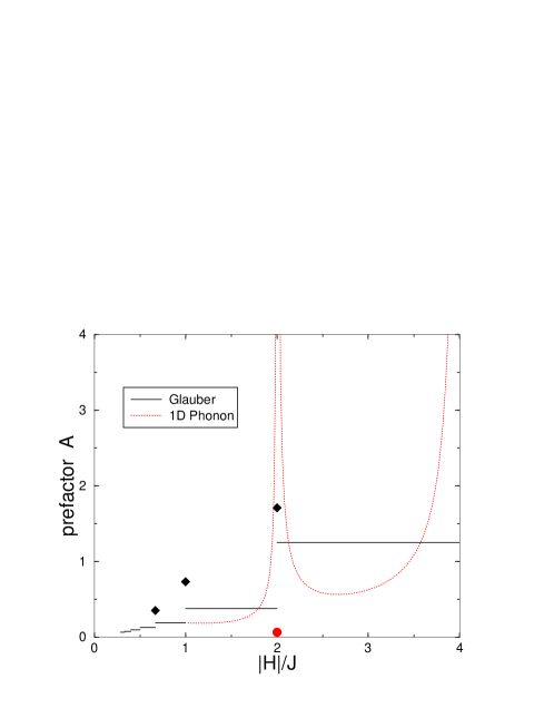
Figure 2: The low-temperature square-lattice prefactors are shown vs. $|H|$. The solid lines and diamonds are the exact low-temperature results for the prefactors for the Glauber dynamic. The dashed curve and filled circle are the low-temperature prefactors for the Ising model with each spin connected to a $d=1$ phonon bath. The curves and lines are derived analytically, while the symbols are from low-temperature MCAMC simulations. The prefactors are shown only for large values of $|H|$. Only three prefactors for the Glauber dynamic have been obtained at the discontinuity. Only prefactors for $|H|\geq J$ are shown for the phonon dynamic

The exact values of $\Gamma_{2}$ and $A_{2}$ are known, so the MCAMC data at finite temperatures can be compared with these predictions. Figure 3(a) shows that near $|H|=2J$ the predicted lines of $T\ln(\langle\tau\rangle)$ vs. $T$ cross. If the measured lifetimes were to follow these expected curves, it would mean that for $T>0.07J$ the lifetime at a field of $|H|=1.99J$ would be smaller than for a field of $|H|=2.01J$. In other words, there would be regions where the lifetime decreases as the field decreases. As seen in Fig. 3 this does not actually occur. Rather, the low-temperature predictions only agree with the data at lower and lower temperatures as the value of $|H|$ approaches the value $2J/|H|$ where the prefactor has a discontinuity. This is also demonstrated in Fig. 3(b). Note that these MCAMC results using a Glauber dynamic are for $10^{3}$ escapes from the metastable state for a $24\times 24$ square lattice Ising system. The error estimates are from the second moment of $\tau$ obtained from the $10^{3}$ escapes. These error estimates should be viewed as approximate, since the measured second moment most likely deviates substantially from the exact one when only $10^{3}$ escapes are used.

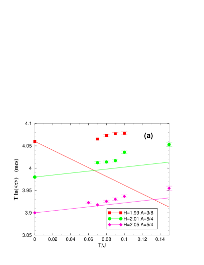
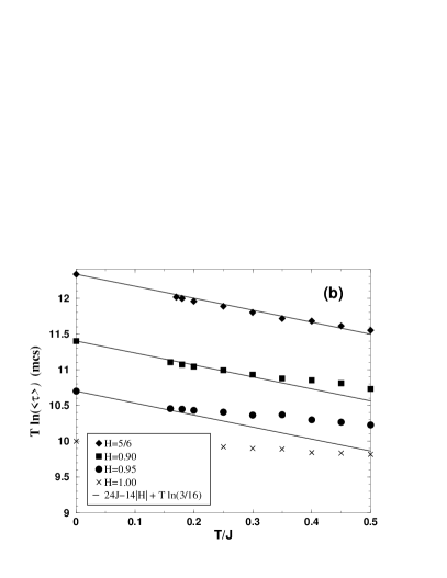
Figure 3: The low-temperature results for the square-lattice Ising model as functions of $T$. The solid lines are the exact low-temperature results, including the prefactors. (a) Three different fields are shown. Note that the lines cross, which would mean a non-monotonic behavior of the lifetime in this region. (b) Results for $\ell_{2}=3$ are shown for several values of $|H|$. Note that as the discontinuity at $|H|$$=$$J$ is approached, the temperature required before the low-temperature results are seen decreases

Figure 4 shows the results for $A_{\rm eff}$ obtained at three different temperatures. Only MCAMC data points in the Single Droplet regime (as defined here by the ratio of the second moment of $\tau$ to $\langle\tau\rangle$ being greater than $1\over 2$ PerSDMD ) are shown. It is seen that the exact low-temperature prefactor is approached at finite temperature more quickly for values of $H$ that are far from the values where $A$ has a discontinuity. Note that in Fig. 4 the higher $|H|$ values start a cross-over toward the multi-droplet regime PerSDMD , and so should not be used in the comparison with the low-temperature prefactors. This cross-over depends on the system size as well as the temperature PerSDMD .

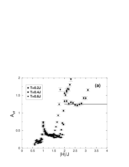
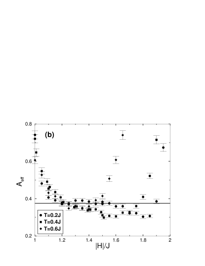
Figure 4: The low-temperature results for the effective prefactor in the Single Droplet regime are shown as a function of $|H|$. The solid horizontal lines are the exact low-temperature prefactors. Three different temperatures are shown. Note that the deviation from the expected results at larger $|H|$ values can be mainly attributed to the cross-over between the Single and Multi-Droplet regimes. (a) For ${1\over 2}J\leq|H|\leq 4J$. (b) Only for $J\leq|H|\leq 2J$, where $\ell_{2}$$=$$2$

Figure 4(b) shows a portion of the data in Fig. 4(a) for $\ell_{2}=2$. Again note that near a value of $H$ where there is a discontinuity (here $|H|=J$ and $2J$) the effective prefactor at finite temperature approaches the exact low-temperature prefactor extremely slowly.

A recent preprint SHNE02 has performed a similar analysis of the prefactors for the square-lattice Ising dynamic using a generalized Becker-Döring approach. The authors find qualitatively similar results to those shown in Fig. 4. However, unlike our results, their results do not approach the predicted low-temperature prefactors. They argue that this might be due to a difference between discrete and continuous times in the Glauber simulations. However, for the temperatures and field values simulated here we did not observe in our simulations that the prefactor value would depend on whether the time in the Glauber simulation is continuous or discrete. In the single-droplet regime relevant at low temperatures, the average lifetimes are extremely long, and consequently the average lifetimes should not depend in a significant way on whether the time in the simulation is continuous or discrete. The dynamic used in ref. SHNE02 is not identical to the Glauber dynamic, and this difference between the two dynamics might account for the difference in the prefactors.

3.2 Phonon Dynamics

For the square-lattice Ising model coupled to a one-dimensional phonon bath Fig. 2 shows the exact low-temperature prefactor KParkCCP for $|H|>J$. This is given by the equation

$$A={{4(2|H|-4J)+(8J-2|H|)}\over{4(2|H|-4J)(8J-2|H|)}}$$ (10)

for $2J<|H|<4J$ and

$$A={{|H|+2(2J-|H|)}\over{2^{4}|H|(2J-|H|)}}$$ (11)

for $J<|H|<2J$ KParkCCP . The same nucleating droplets (except at $|H|=2J$) are responsible for the decay of the metastable state for this dynamic as for the Glauber dynamic, so the same value of $\Gamma_{2}$ is found for both dynamics (except at $|H|=2J$). Note that for this dynamic the prefactor is not constant when $\ell_{2}$ is constant, and there is a divergence in the prefactor when $|H|=2J$ or $|H|=4J$. The divergence in the prefactor at $|H|=2J$ is due to the nucleating droplet at this field being two next-nearest neighbor overturned spins that has $\Gamma=8J$ rather than the value $\Gamma_{2}=4J$ for the Glauber dynamic. Recently, such a divergence in the prefactor has also been found in a model with continuous degrees of freedom MaiStePRL . Figure 5 shows values of $A_{\rm eff}$ (from finite-temperature MCAMC) at two different temperatures as they approach the exact low-temperature results. Note that the divergence in the prefactor is only seen at lower temperatures.

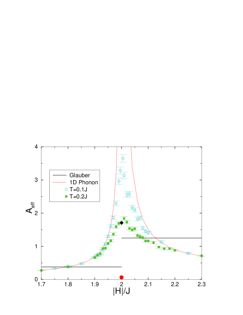
Figure 5: The low-temperature results for the prefactors vs. $|H|$. The solid lines and diamond are the exact low-temperature results for the prefactors for the Glauber dynamic. The dashed curve and filled circle are the low-temperature prefactor for the Ising model with each spin connected to a $d=1$ phonon bath. The curves and lines are derived analytically, while the symbols are from low-temperature Monte Carlo simulations. The effective prefactor from MCAMC data near $H=2J$ is shown for $10^{3}$ escapes from the metastable state on a $32\times 32$ lattice at $T=0.1J$ and $T=0.2J$. Note that the low-temperature results are approached very slowly near the discontinuity

4 Simple-cubic lattice Ising Model

For the kinetic Ising model with the Glauber dynamic on a simple cubic lattice the average lifetime in the low-temperature limit (for fixed $H$ and system size) is given by $\langle\tau\rangle=A_{3}\exp(\beta\Gamma_{3})/q$ with

$$\Gamma_{3}=12J\ell_{3}^{2}-8J\ell_{3}-2|H|\ell_{3}^{2}(\ell_{3}-1)+\Gamma_{2}$$ (12)

with $\ell_{3}=\lfloor 4J/|H|\rfloor+1$ RecPref ; CFQ1 ; CFQ2 and $\Gamma_{2}$ the square-lattice nucleating droplet energy defined above. Equation (12) should be valid when $|H|\leq 4J$ and $2J/|H|$ is not an integer. The number of spins in the nucleating droplet is $n_{c}=\ell_{3}^{2}(\ell_{3}-1)+(\ell_{2}^{2}-\ell_{2}+1)$. The nucleating droplet is a cube with $\ell_{3}$ overturned spins per side, with one face removed and the appropriate square-lattice nucleating droplet placed where the face was removed. Figure 6 shows a nucleating droplet for $J\leq|H|\leq 2J$, so $\ell_{3}=3$ and $\ell_{2}=2$, and the nucleating droplet has $n_{c}=21$. For this value of $H$ the square-lattice nucleating droplet consists of three overturned spins in an L-shape.

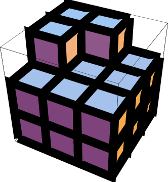
Figure 6: A low-temperature nucleating droplet with $\ell_{3}=3$ and $\ell_{2}=2$. It consists of a cube of overturned spins with sides of length $\ell_{3}$, with the spins from one face removed and a nucleating droplet with $\ell_{2}$ placed on the removed face

The prefactor for the simple cubic lattice with the Glauber dynamic has recently been found to be $A_{3}=\left[16(\ell_{3}-\ell_{2}+1)(\ell_{2}-1)\right]^{-1}$ for $\ell_{3}\geq 3$ RecPref . The low-temperature prefactor for $\ell_{3}=2$ (so $2J<|H|<4J$) has not yet been derived, being a straightforward but lengthy calculation. The low-temperature prefactor for $\ell_{3}=1$ (so $4J<|H|<6J$) is easily derived to be $A_{3}=7/6$.

Figure 7(a) shows the expected low-temperature result near $|H|=2J$ for the simple cubic Ising model as a function of $|H|$. Projective dynamics MANreview ; MiroPRL ; Granada simulation results are also shown for $T=0.2T_{\rm c}$. The critical temperature is $T_{\rm c}\approx 4.51J$. If the prefactor were unity, the expected low-temperature result (solid line) would be independent of temperature. For other prefactors, the dashed line is adjusted so the result with the prefactor depends on $T$. The simulation data are for a $32^{3}$ Ising system using a projective dynamic method MANreview ; MiroPRL . Note that away from a discontinuity the simulation data fall quite nicely on the expected low-temperature results including the predicted prefactor. However, they do not follow the expected results near the discontinuities (where $\ell_{3}$ changes). Shown here is only the discontinuity near $|H|=2J$. This is similar to the result found in the square-lattice model. Namely, how low in temperature the simulation must be performed before the low-temperature result is valid depends strongly on how close one is to a discontinuity in the low-temperature prefactor.

Note that, as seen in Eq. (12) and in Fig. 7(a), there is a discontinuity in $\Gamma_{3}$ whenever $\ell_{3}$ changes. For all values of $H$ where $\ell_{3}$ changes the discontinuity is such that $\Gamma_{3}$ decreases by $4J$. If the data were to follow these low-temperature results, as $|H|$ decreases through one of these discontinuities the average lifetime would decrease. This would occur not just because of a discontinuity in the prefactor, as in the square-lattice Ising model, but also because of a discontinuity in the exponential (in $\Gamma_{3}$).

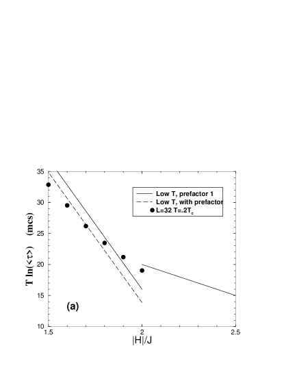
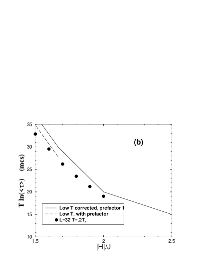
Figure 7: The low-temperature results for the simple cubic lattice vs. $|H|$. The dashed line includes known exact prefactors. The symbols are projective dynamics simulation results on a $32^{3}$ lattice at $T=0.2T_{\rm c}$. (a) The solid lines are the exact low-temperature results RecPref ; CFQ1 ; CFQ2 . (b) The solid lines are the exact, corrected, low-temperature results. The dashed line shows the known exact prefactors, which in this figure are only known for $|H|<{5\over 3}J$. Note that now the exponential portion of the low-temperature prediction is continuous

Figure 8 shows MCAMC simulation results using the Glauber dynamic for the simple-cubic Ising model at $|H|=3.5J$. For this value of $H$ one has $\ell_{3}=2$ and $\ell_{2}=1$ so the nucleating droplet is predicted to have $n_{c}=5$ overturned spins, and the predicted value of $\Gamma_{3}=5J$. The low-temperature prefactor is not known for this value of $H$. As seen in Fig. 8, the low-temperature MCAMC data do not tend toward $\Gamma_{3}=5J$, but could reasonably tend toward $\Gamma_{3}=7J$. The published low-temperature predictions RecPref ; CFQ1 ; CFQ2 do not agree with our MCAMC results.

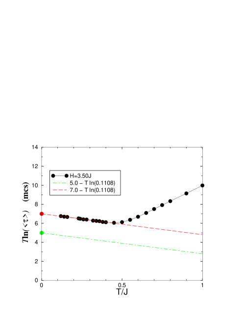
Figure 8: The low-temperature results for the simple cubic lattice as a function of $T$ for $|H|=3.5J$. The lines have a slope of the best fit to the low-temperature data. The results at $T=0$ are the exact low-temperature results, both the uncorrected ones (lower point) and the corrected ones (upper point)

The reason for this disagreement is that the previously reported low-temperature predictions are incomplete: they give accurate values for $\Gamma_{3}$ from Eq. (12) for some but not all values of $H$. This is because the most probable path of escape from the metastable state has a droplet with higher energy than predicted by $\Gamma_{3}$ from Eq. (12) for some values of $H$. For $3J\leq|H|\leq 4J$ this higher energy saddle has an energy of $28J-6|H|$, that corresponds to three overturned spins in an L-shape, and so has $n_{c}=3$. For all $|H|<4J$ this droplet lies along the most probable path to the saddle point, but it is the highest energy point along this path only for $3J\leq|H|\leq 4J$, and hence is then the critical nucleating droplet. This scenario predicts that for $|H|=3.5J$ one should have $\Gamma_{3}=7J$, in agreement with the MCAMC results shown in Fig. 8.

Similar results hold near other values of $H$ where $\ell_{3}$ changes. For example, near $|H|=2J$ the low-temperature predictions RecPref ; CFQ1 ; CFQ2 are that for $n_{c}=5$ ($2J<|H|<4J$) one has $\Gamma_{3}=40J-10|H|$ and for $n_{c}=21$ ($J<|H|<2J$) one has $\Gamma_{3}=100J-42|H|$ (Fig. 6). However, there is a droplet with 15 overturned spins consisting of $2$$\times$$2$$\times$$3$ overturned spins with a $\ell_{2}=2$ droplet of overturned spins on one of the $2$$\times$$3$ faces. This 15-spin droplet has $\Gamma=80J-30|H|$. This is the nucleating droplet for values of $H$ when this $\Gamma$ is larger than the predicted values of $\Gamma_{3}$ for $n_{c}=5$ or $n_{c}=21$. This occurs for ${5\over 3}J<|H|<2J$. At $|H|=2J$ the droplets with 5 and with 15 overturned spins have the same energy, while at $|H|={5\over 3}J$ the droplets with 15 and with 21 overturned spins have the same energy. The correct predicted values of $\Gamma_{3}(H)$ are hence continuous when this droplet with 15 overturned spins is included. This is shown in Fig. 7(b). In general, one can show that all the predicted RecPref ; CFQ1 ; CFQ2 discontinuities in $\Gamma_{3}$ where $\ell_{3}$ changes vanish. After this study was completed another paper describing the low-temperature properties of the simple cubic dynamic Ising model EJP96 was brought to the author’s attention. In ref. EJP96 it is shown that the critical droplet size is $n_{c}=\ell_{3}(\ell_{3}-\delta)(\ell_{3}-1)+(\ell_{2}^{2}-\ell_{2}+1)$ where $\delta$$=$$0$ unless $4J+\sqrt{16J^{2}+|H|^{2}}<|H|(2\ell_{3}-1)$ in which case $\delta$$=$$1$. For the simple cubic lattice, the critical value of $\Gamma_{3}(H)$ is thus continuous for all $H$, just as for the square lattice.

5 Summary and Conclusions

From long-time simulations of kinetic Ising models, the question of when the low-noise limit results are approached by finite-temperature simulations has been addressed. In particular, we have studied the limit where the system size and $H$ are fixed, while the temperature is lowered. There are three main features that emerge:

• The square-lattice and simple-cubic-lattice low-temperature predictions have the form $\langle\tau\rangle=A\exp(\beta\Gamma)$ with $\Gamma(H)$ continuous almost everywhere, but with $A(H)$ discontinuous.

• The finite-temperature simulation results must be at a lower temperature to see the low-temperature predictions if the applied field is near a value where the low-temperature prefactor has a discontinuity or a divergence.

• The finite-temperature results have average lifetimes $\langle\tau\rangle$ which are decreasing functions of $|H|$. This is true even if the low-temperature results are not always decreasing as $|H|$ increases.

We have shown that these features are true for simulations in the square-lattice and simple-cubic-lattice kinetic Ising model with various dynamics. Whether or not these features of $\langle\tau\rangle$ can be shown to be true in general is an interesting question for future research.

Acknowledgements
Special thanks to M. Kolesik for allowing inclusion of unpublished projective dynamic data. Thanks to P.A. Rikvold and K. Park for many useful discussions. Partially funded by NSF DMR-0120310. Supercomputer time provided by the DOE through NERSC.

References

- (1) N.G. van Kampen, Stochastic Processes in Physics and Chemistry (Elsevier Science, Amsterdam, 1982)
- (2) J.A. Bucklew, Large Deviaion Techniques in Decision, Simulation, and Estimation (Wiley, New York, 1990)
- (3) R.J. Glauber: J. Math. Phys. 4, 294 (1963)
- (4) K. Park, M.A. Novotny, Comp. Phys. Commun. in press; e-print cond-mat/0109214
- (5) K. Park, M.A. Novotny, in: Computer Simulation Studies in Condensed Matter Physics XIV, ed. by D.P. Landau, S.P. Lewis, H.-B. Shüttler (Springer-Verlag, Berlin), in press
- (6) K. Blum, Density Matrix Theory and Applications, second edition (Plenum Press, New York, 1996), Chapter 8
- (7) K. Binder, E. Stoll, Phys. Rev. Lett. 31, 47 (1973); K. Binder, H. Müller-Krumbhaar, Phys. Rev. B 9, 2328 (1974)
- (8) Ph.A. Martin: J. Stat. Phys. 16, 149 (1977)
- (9) P.A. Rikvold, H. Tomita, S. Miyashita, S.W. Sides, Phys. Rev. E 49, 5080 (1994); P.A. Rikvold, B.M. Gorman, in Annual Reviews of Computational Physics I, ed. by D. Stauffer (World Scientific, Singapore, 1994), p. 149
- (10) V.A. Shneidman, G.M. Nita, e-print cond-mat/0201064
- (11) A.B. Bortz, M.H. Kalos, J.L. Lebowitz: J. Comput. Phys. 17, 10 (1975)
- (12) M.A. Novotny: Comp. in Phys. 9, 46 (1995)
- (13) M.A. Novotny: Phys. Rev. Lett. 74, 1 (1995); erratum 75, 1424 (1995).
- (14) M.A. Novotny: in: Computer Simulation Studies in Condensed Matter Physics IX, ed. by D.P. Landau, K.K. Mon, H.-B. Shüttler (Springer-Verlag, Berlin, Heidelberg, 1997), p. 182
- (15) M. A. Novotny, Comp. Phys. Commun., in press; e-print cond-mat/0108429
- (16) M.A. Novotny: in Annual Reviews of Computational Physics IX, ed. by D. Stauffer (World Scientific, Singapore, 2001), p. 153
- (17) E. Jordão Neves, R.H. Schonmann: Commun. Math. Phys. 137, 209 (1991)
- (18) A. Bovier, F. Manzo: e-print cond-mat/0107376
- (19) R.S. Maier, D.L. Stein, Phys. Rev. Lett. 87 022301 (2001)
- (20) D. Chen, J. Feng, M. Qian: Science in China (Series A) 40, 832 (1997)
- (21) D. Chen, J. Feng, M. Qian: Science in China (Series A) 40, 1129 (1997)
- (22) M. Kolesik, M.A. Novotny, P.A. Rikvold: Phys. Rev. Lett. 80, 3384 (1998)
- (23) M.A. Novotny, M. Kolesik, P.A. Rikvold, Comp. Phys. Commun. 121-122, 303 (1999)
- (24) G. Ben Arous, R. Cerf, Electronic J. Prob. 1, 1 (1996)