[

Essential Role of the Cooperative Lattice Distortion in the Charge, Orbital and Spin Ordering in doped Manganites

Abstract

The role of lattice distortion in the charge, orbital and spin ordering in half doped manganites has been investigated. For fixed magnetic ordering, we show that the cooperative lattice distortion stabilize the experimentally observed ordering even when the strong on-site electronic correlation is taken into account. Furthermore, without invoking the magnetic interactions, the cooperative lattice distortion alone may lead to the correct charge and orbital ordering including the charge stacking effect, and the magnetic ordering can be the consequence of such a charge and orbital ordering. We propose that the cooperative nature of the lattice distortion is essential to understand the complicated charge, orbital and spin ordering observed in doped manganites.

]

The unusual charge, orbital and spin ordering (COSO) in manganites have recently attracted much attention [1, 2, 3, 4, 5, 6, 7, 8, 9, 10, 11]. In some of these materials such as Pr_1/2Ca_1/2MnO₃ [1], La_1/2Sr_3/2MnO₄ [2, 3] and La_1/3Ca_2/3MnO₃ [4], below a certain temperatures $T_{CO}$, electronic carriers become localized onto specific sites, which display long-range order throughout the crystal structure (charge ordering). Meanwhile the filled Mn³⁺ $e_{g}$ orbitals also develop long-range order (orbital ordering). When the temperature is further decreased to a much lower temperature $T_{N}$, an antiferromagnetic (AF) magnetic ordering with a zigzag pattern sets in (Fig. 1(a)). In some others like La_1/2Ca_1/2MnO₃ [5] and Nd_1/2Sr_1/2MnO₃ [7], the system first undergoes a ferromagnetic (FM) transition at the Curie temperature $T_{C}$, then enters into the CE-type charge, orbital and spin ordering (COSO) state at a lower temperature $T_{CO}=T_{N}$. Theoretically, it has been proposed that the charge and orbital ordering (COO) in half-doped manganites has a magnetic spin origin [8, 9]. However, such a theory can not be applied to those materials with $T_{CO}>T_{N}$, where the COO is established before the spin ordering. Even for those whose $T_{CO}=T_{N}$, it has been shown that in a pure electronic model, the on-site repulsion $U$ destabilizes the CE structure towards the rod-type (C-type) AF state (Fig. 1(b)) in realistic parameter regime of $U$ [12]. Yunoki et al. [10] considered the effects of lattice distortions (LD), and found that both the noncooperative LD (NLD) and cooperative LD (CLD) can lead to the CE-type COSO. In their work $U$ is neglected and the calculation was performed on a $4\times 4\times 2$ lattice where the size effect is prominent. Since in the absence of $U$ the CE state can be obtained without LD [8, 9], the role of LD seems not very clear there. It is desirable to clarify what the LD results for the CE state would be destabilized by $U$.

In this work, we investigate the role of LD and large $U$ in the COSO in half doped manganites. For fixed magnetic ordering, by studying the competition between the CE and C states, we found that only CLD can stabilize the CE state in the presence of large $U$. Furthermore, without invoking the magnetic interactions, the CLD alone can lead to the experimentally observed COO, including the charge stacking effect. The magnetic ordering is the consequence of such a COO.

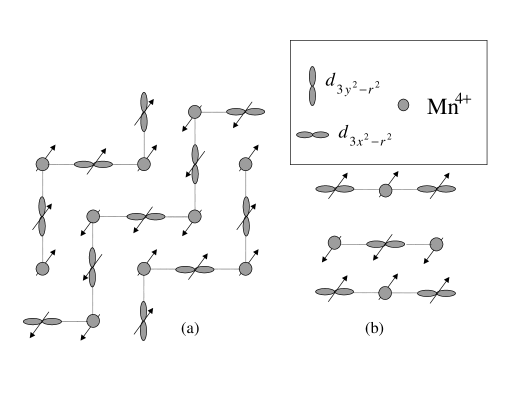
FIG. 1.: View of the (a) CE and (b) C phase in the x-y plane. The arrows refers to the spin. Along the z-direction neighboring sites have the same charge and orbital states but opposite spins.

The interaction concerning the lattice freedom includes two parts: $H_{lat}=H_{ep}+H_{ela}$. $H_{ep}$ is the coupling between lattice distortion and $e_{g}$ electrons, given by[13, 14]

$$H_{ep}=-\frac{3\lambda}{\sqrt{6}}\sum_{i\gamma\gamma^{\prime}}c^{\gamma{\dagger}}_{i}(\sqrt{2}\beta Q_{1i}\hat{{\bf 1}}+Q_{2i}\sigma_{x}+Q_{3i}\sigma_{z})_{\gamma\gamma^{\prime}}c^{\gamma^{\prime}}_{i},$$ (1)

where $\sigma_{x},\sigma_{z}$ are Pauli matrices, $c_{i}^{\gamma}$ is electron operator of orbital $\gamma$ ($z=d_{3z^{2}-r^{2}},\bar{z}=d_{x^{2}-y^{2}}$), and $Q_{1i}=\frac{1}{\sqrt{3}}(v^{x}_{i}+v^{y}_{i}+v^{z}_{i}),Q_{2i}=\frac{1}{\sqrt{2}}(v^{y}_{i}-v^{x}_{i}),Q_{3i}=\frac{1}{\sqrt{6}}(2v_{i}^{z}-v^{x}_{i}-v^{y}_{i})$ are the breathing ($Q_{1i}$) and Jahn-Teller ($Q_{2i}$, $Q_{3i}$) modes of the LD. Here $v^{\alpha}_{i}=u^{\alpha}_{i+\hat{\alpha}}-u^{\alpha}_{i-\hat{\alpha}}$, with $u^{\alpha}_{i\pm\hat{\alpha}}$ being the $\alpha$-component of the displacements from the equilibrium position of the neighboring oxygen ion in the $\pm\alpha$ direction. The parameter $\beta$ is expected close to 1/2 [14]. The index of spin has been omitted, which is always parallel to the local spin due to the strong Hund’s coupling. Throughout the paper, we use $\alpha=x,y$ or $z$ to denote either the direction or the orbital state, in the latter case it refers to the orbital $d_{3\alpha^{2}-r^{2}}$, whose orthogonal state is denoted as $\bar{\alpha}$. There are relationships $c_{i}^{x,y}=c_{i}^{z}/2\mp\sqrt{3}c_{i}^{\bar{z}}/2$ and $c_{i}^{\bar{x},\bar{y}}=\pm\sqrt{3}c_{i}^{z}/2+c_{i}^{\bar{z}}/2$. $H_{ela}$ is the elastic energy and depends on the relative displacements of neighboring atoms with respect to the ideal perovskite lattice. In a unit cell of the perovskite A_1-xA${}^{\prime}_{x}$MnO₃, there are three kinds of atoms: Mn, O and Z(=A or A^′). The main contribution to $H_{ela}$ may include the elastic energies of the neighboring Mn-O, O-Z and Mn-Z atoms. Up to now no studies concerning the elastic energy of Z atoms has been made, however, this energy should be important, as without it the Z atoms can have arbitrary displacement instead of sitting in the center of the cubic cell cornered by eight Mn ions, and experimental observations indicate that the Z atoms also participate in the LD [5]. In harmonic approximation, the elastic energy of the CLD may be written as

$$H_{ela} = \frac{K_{1}}{2}\sum_{i,\kappa}[(\boldmath{\mbox{$\delta$}}_{i}-{\bf u}_{i,\kappa})\cdot{\bf e}_{\kappa}]^{2}+\frac{K_{2}}{2}\sum_{i,\xi}[(\boldmath{\mbox{$\Delta$}}_{i}-{\bf u}_{i,\xi})\cdot{\bf e}_{\xi}]^{2}$$ (2)

$$+\frac{K_{3}}{2}\sum_{i,\eta}[(\boldmath{\mbox{$\Delta$}}_{i}-\boldmath{\mbox{$\delta$}}_{i,\eta})\cdot{\bf e}_{\eta}]^{2},$$ (3)

where $\boldmath{\mbox{$\delta$}},{\bf u}$ and $\Delta$ are the dimensionless displacements of the Mn, O and Z ions with reference to the ideal perovskite lattice, ${\bf e}_{\kappa}$, ${\bf e}_{\xi}$ and ${\bf e}_{\eta}$ are unit vectors along the directions of neighboring Mn-O, Z-O and Z-Mn, respectively, with $\kappa,\xi$ and $\eta$ the indices of neighbors. In principle, the spring constants between Z-O and Z-Mn depend on whether Z=A or A^′, here to simplify our study we replace them by the averaged $K_{2}$ and $K_{3}$. Since the distance between these neighboring atoms are $L_{\mbox{{Mn-O}}}<L_{\mbox{{O-Z}}}<L_{\mbox{{Z-Mn}}}$, one expects that the spring constants $K_{1}>K_{2}>K_{3}$.

In the classical treatment of the LD [10, 13], the displacements of various sites are determined by minimizing the total energy of the system, $\partial H_{lat}/\partial w_{i}^{\alpha}=0$, where $w_{i}^{\alpha}$ ($w=\delta,\Delta$ or $u$) is the $\alpha$-component of the displacement. For harmonic $H_{ela}$, such a calculation can be easily performed in the momentum space to get the optimized values of the displacements. Then after substituting these displacements into Eqs.(1) and (3), $H_{lat}$ reduces to

$$H_{lat}^{eff}=-\epsilon_{l}\sum_{{\bf q},\alpha\alpha^{\prime}}f_{{\bf q}}^{\alpha{\dagger}}G_{\alpha\alpha^{\prime}}({\bf q})f_{{\bf q}}^{\alpha^{\prime}},$$ (4)

where $\epsilon_{l}=\lambda^{2}/K_{1}$, $f_{{\bf q}}^{\alpha}$ is the Fourier transform of $f_{i}^{\alpha}=\beta n_{i}+m_{i}^{\alpha}$, with $n_{i}=n_{i}^{\alpha}+n_{i}^{\bar{\alpha}}$ and $m_{i}^{\alpha}=n_{i}^{\alpha}-n_{i}^{\bar{\alpha}}$, and $n_{i}^{\alpha(\bar{\alpha})}=c_{i}^{\alpha(\bar{\alpha}){\dagger}}c_{i}^{\alpha(\bar{\alpha})}$. The tensor $G=P+DR^{-1}W$, where $P,D,R$ and $W$ are $3\times 3$ matrices, with $P_{\alpha\alpha^{\prime}}=\delta_{\alpha\alpha^{\prime}}(3K_{1}+4K_{3})S_{\alpha}^{2}/(3K_{1}S_{\alpha}^{2}+4K_{3})$, $D_{xx}=h_{x}C,D_{xy}=-S_{xy}h_{x}C_{z},W_{xx}=3K_{1}h_{x}C,W_{xy}=-3K_{1}S_{x}S_{y}^{2}C_{yz},R_{xx}=4K_{3}(1-C^{2}H_{x}-C_{z}^{2}S_{xy}^{2}H_{y}-C_{y}^{2}S_{xz}^{2}H_{z})+3K_{2}(2-C_{xy}^{2}-S_{xy}^{2}-C_{xz}^{2}-S_{xz}^{2}),R_{xy}=C_{xy}S_{xy}[4K_{3}(C_{z}^{2}H_{x}+C_{z}^{2}H_{y}-S_{z}^{2}H_{z})+6K_{2}]$, where $S_{\alpha}=\sin(q_{\alpha}/2)$ and $C_{\alpha}=\cos(q_{\alpha}/2)$, $S_{\alpha\alpha^{\prime}}=S_{\alpha}S_{\alpha^{\prime}}$ and $C_{\alpha\alpha^{\prime}}=C_{\alpha}C_{\alpha^{\prime}}$, $C=C_{x}C_{y}C_{z}$, $H_{\alpha}=4K_{3}/(3K_{1}S_{\alpha}^{2}+4K_{3})$ and $h_{\alpha}=H_{\alpha}S_{\alpha}C_{\alpha}$. The other elements of $D,R$ and $W$ can be obtained by exchanging the indices, e.g., $D_{yy}=h_{y}C$ and $D_{yx}=-S_{xy}h_{y}C_{z}$, etc. The displacements are connected to $G$ through $u_{{\bf q},\alpha}^{\alpha}=-i\lambda\sum_{\alpha^{\prime}}G_{\alpha\alpha^{\prime}}({\bf q})\langle f_{{\bf q}}^{\alpha^{\prime}}\rangle/S_{\alpha}$ and $\delta_{{\bf q}}^{\alpha}=u_{{\bf q},\alpha}^{\alpha}-i\lambda\tan(q_{\alpha}/2)\langle f_{{\bf q}}^{\alpha}\rangle/K_{1}$, with ${\bf u}_{{\bf q},\alpha}$ being the Fourier transform of ${\bf u}_{i+\hat{\alpha}}$, and $\boldmath{\mbox{$\Delta$}}_{{\bf q}}$ is a function of ${\bf u}_{{\bf q},\alpha}$ and $\boldmath{\mbox{$\delta$}}_{{\bf q}}$. It should be pointed out that the form of Eq.(4) is actually general for $H_{lat}$ with any harmonic $H_{ela}$, and different choice of $H_{ela}$ leads to different $G$. For example, the $H_{ela}$ in Ref. REFERENCES includes $K_{1}$ and $K_{1}^{\prime}$ (the spring constant between neighboring Mn sites) terms, where the $G$ tensor is $G^{(1)}_{\alpha\alpha^{\prime}}({\bf q})=\delta_{\alpha\alpha^{\prime}}(K_{1}+2K_{1}^{\prime}S^{2}_{\alpha})/(K_{1}+2K_{1}^{\prime})$. While in Refs. REFERENCES and REFERENCES, NLD and CLD yield $G^{(2)}_{\alpha\alpha^{\prime}}=\delta_{\alpha\alpha^{\prime}}$ and $G^{(3)}_{\alpha\alpha^{\prime}}({\bf q})=S_{\alpha}^{2}\delta_{\alpha\alpha^{\prime}}$, respectively. Here the difference between CLD and NLD is whether the $G$ tensor depends on ${\bf q}$ or not.

FIG. 2.: Calculated $g_{0},g_{1},g_{2}$ and $g_{1}^{\prime}$ as a function of $K_{2}/K_{1}$, with fixed $K_{3}/K_{2}=0.5$.

Eq.(4) indicates that LD results in an effective electronic interaction. In real space, it is

$$H_{lat}^{eff}= - \epsilon_{l}\{\sum_{i,\alpha}[g_{0}f_{i}^{\alpha}f_{i}^{\alpha}-g_{1}f_{i}^{\alpha}f_{i+\hat{\alpha}}^{\alpha}-g_{2}f_{i}^{\alpha}f_{i+2\hat{\alpha}}^{\alpha}$$ (5)

$$+ g_{1}^{\prime}\sum_{\alpha^{\prime}(\neq\alpha)}f_{i}^{\alpha^{\prime}}f_{i+\hat{\alpha}}^{\alpha^{\prime}}]+{\sum_{ij,\alpha\alpha^{\prime}}}^{\prime}G_{\alpha\alpha^{\prime}}^{ij}f_{i}^{\alpha}f_{j}^{\alpha^{\prime}}\},$$ (6)

where the sum $\sum^{\prime}$ includes all the other terms. $g_{1}^{\prime}$ is found to be smaller than the coupling coefficients of the first several $f_{i}^{\alpha}f_{i+n\hat{\alpha}}^{\alpha}$ terms, but larger than any other coefficients $G_{\alpha\alpha^{\prime}}^{ij}$. Fig. 2 shows the calculated values of $g_{0},g_{1},g_{2}$ and $g_{1}^{\prime}$. From Eq.(6), the main effects of the CLD corresponds to an effective short-range orbital-dependent coupling between occupied Mn sites. If $G$ is replaced by $G^{(i)}$ (i=1,2,3), then in the CLD cases of $G^{(1)}$ and $G^{(3)}$, there are only the $g_{0}$ and $g_{1}$ terms, while in the NLD case of $G^{(2)}$, there is only the $g_{0}$ term.

Now let us investigate the effect of LD to the COSO at half doping. First we see the case with fixed CE-type spin ordering. In the one-dimensional zigzag FM chain (see Fig. 1(a)), the double-exchange (DE) Hamiltonian reduces to

$$H_{DE} = \sum_{i=\mbox{even}}[d_{Bi}^{{\dagger}}(t_{1}c_{C,i+1}+t_{2}c_{C,i-1})+\mbox{H.c.}]$$ (7)

$$+U(n_{Bi}n_{Bi}^{\prime}+n_{C,i+1}^{z}n_{C,i+1}^{\bar{z}}),$$ (8)

where $d_{Bi}=c_{i}^{x}$ and $c_{i}^{y}$ for $i=4j$ and $4j+2$ (j is an integer), $c_{Ci}=(c_{i}^{z},\pm c_{i}^{\bar{z}})^{T}$ for i=$4j+1$ and $4j+3$, and $i=$even and odd corresponds to the bridge (Mn³⁺) and corner (Mn⁴⁺) sites, respectively, $t_{1,2}=-(t/2,\pm\sqrt{3}t/2)$, $n_{Bi}=d_{Bi}^{{\dagger}}d_{Bi}$ and $n_{Bi}^{\prime}=d_{Bi}^{\prime{\dagger}}d_{Bi}^{\prime}$, with $d_{Bi}^{\prime}$ being the orthogonal state of orbital $d_{Bi}$, and $n_{Ci}^{\gamma}=c_{Ci}^{\gamma{\dagger}}c_{Ci}^{\gamma}$. In realistic manganites, the parameter regime of the on-site repulsion $U=10\sim 20t$, so that the system is strong correlated. In this regime double occupancy of electrons at a site is almost forbidden, and it is appropriate to use the Gutzwiller projection (GP) method, valid for $U\rightarrow\infty$ [9], to take into account such a strong correlation effect. In GP we introduce constrained electrons at each site. Each electron operator in Eq.(8) is replaced by the corresponding projected operator to eliminate the double occupancy, $d_{Bi}\rightarrow(1-n_{Bi}^{\prime})d_{Bi}$ and $c_{Ci}^{\gamma}\rightarrow(1-n_{i}^{\bar{\gamma}})c_{Ci}^{\gamma}$ ($\bar{\gamma}=\bar{z}(z)$ when $\gamma=z(\bar{z})$). Then we use a mean-field approximation by decoupling the high order terms such as $c_{Bi}^{x{\dagger}}c_{C,i+1}^{z}n_{i+1}^{\bar{z}}\rightarrow c_{Bi}^{x{\dagger}}c_{C,i+1}^{z}\langle n_{i+1}^{\bar{z}}\rangle+\langle c_{Bi}^{x{\dagger}}c_{C,i+1}^{z}\rangle n_{i+1}^{\bar{z}}$. After a Fourier transform, we have

$$H_{DE}^{MF} = \sum_{k\gamma}(d_{Bk}^{{\dagger}}\tilde{t}_{k}^{\gamma}c_{Ck}^{\gamma}+c_{Ck}^{\gamma{\dagger}}\tilde{t}_{k}^{\gamma\ast}d_{Bk}+\epsilon_{\gamma}c_{Ck}^{\gamma{\dagger}}c_{Ck}^{\gamma})$$ (9)

$$+\sum_{k}\epsilon^{\prime}d_{Bk}^{\prime{\dagger}}d_{Bk}^{\prime}+E^{0}_{DE},$$ (10)

where $\tilde{t}_{k}^{\gamma}=\langle 1-n_{B}^{\prime}\rangle\langle 1-n_{C}^{\bar{\gamma}}\rangle t_{k}^{\gamma}$ with $t_{k}^{z}=-t\cos k$ and $t_{k}^{\bar{z}}=t\sqrt{3}i\sin k$, $\epsilon_{\gamma}=-2\langle 1-n_{B}^{\prime}\rangle\mbox{Re}\sum_{k}\langle d_{Bk}^{{\dagger}}t_{k}^{\bar{\gamma}}c_{Ck}^{\bar{\gamma}}\rangle$, $\epsilon^{\prime}=-2\mbox{Re}\sum_{k\gamma}\langle 1-n_{C}^{\bar{\gamma}}\rangle\langle d_{Bk}^{{\dagger}}t_{k}^{\gamma}c_{Ck}^{\gamma}\rangle$, and $E^{0}_{DE}$ is the MF energy constant.

For $H_{lat}$ of Eq.(4), in the case of CE type spin ordering the sum over ${\bf q}$ includes ${\bf q}=(0,0,0),\pm(\pi/2,\pi/2,0)$ and $(\pi,\pi,0)$, and can be denoted as $q=0,\pm\pi/2$ and $\pi$ in the 1D FM chain. By decoupling the quartic term $f_{q}^{\alpha{\dagger}}f_{q}^{\alpha^{\prime}}\rightarrow\langle f_{q}^{\alpha{\dagger}}\rangle f_{q}^{\alpha^{\prime}}+f_{q}^{\alpha{\dagger}}\langle f_{q}^{\alpha^{\prime}}\rangle$, Eq.(4) reduces to

$$H_{lat}^{MF}=\sum_{k,q}(c_{k-q}^{{\dagger}}D_{q}c_{k}+\mbox{H.c.})+E^{0}_{lat},$$ (11)

where $c_{k}$ is the Fourier transform of $c_{i}=(c_{i}^{z},c_{i}^{\bar{z}})^{T}$ and $D_{q}=-\epsilon_{l}\sum_{\alpha\alpha^{\prime}}G_{\alpha\alpha^{\prime}}(q)\langle f_{q}^{\alpha^{\prime}{\dagger}}\rangle F^{\alpha}$, with $F^{\alpha}=\beta+\cos\phi_{\alpha}\sigma_{z}+\sin\phi_{\alpha}\sigma_{x}$ and $\langle f_{q}^{\alpha{\dagger}}\rangle=\sum_{k}\langle c_{k+q}^{{\dagger}}F^{\alpha}c_{k}\rangle$.

FIG. 3.: Energy per site in CE (solid line) and C (dotted line) states as a function of $\epsilon_{l}/t$ and the corresponding charge disproportionation with (a) $G^{(1)}$, (b) $G^{(2)}$, (c) $G^{(3)}$ and (d) $G$, with $\beta=0.5$. In $G^{(1)}$ $K_{1}^{\prime}/K_{1}=0.5$, and in $G$ $K_{2}=2K_{3}=0.4K_{1}$.

The full Hamiltonian $H=H_{DE}^{MF}+H_{lat}^{MF}$ can be solved by iteration. In the next we will make a comparison of the magnetic CE and C states. These two states have the same magnetic energy $-J_{AF}$ per site, where $J_{AF}$ is the AF magnetic superexchange between neighboring local spins, so that the relative stability of them is independent of the parameter $J_{AF}$. While other magnetic states, say, the FM and layered (A)-type AF states, have different magnetic energies so that their stabilities depend on $J_{AF}$, and become less stable with respect to the CE and C state when $J_{AF}$ increases. In the C state there is only one effective orbital in each site so that $U$ has no effect and $H_{DE}=-t\sum_{k}c_{k}^{x{\dagger}}c_{k}^{x}$ in the x-orientated FM chain. Such a property make the competition between the C and CE states alone very interesting. In the absence of the electron-lattice interaction, without $U$ the energy per site is $E^{CE}=-0.693t$ and $E^{C}=-0.637t$, when $U$ increases $E^{C}$ keeps unchanged while $E^{CE}$ increases and becomes higher than $E^{C}$ at about $U=5t$ [12], indicating that the strong electronic correlation would destabilize the CE phase towards the C state. When the electron-lattice interaction is taken into account, Fig. 3 shows the energy per site and the charge disproportionation $d_{c}=\langle n_{2j}-n_{2j+1}\rangle$ as a function of $\epsilon_{l}/t$ in the CE and C states. Fig. 3 (a-d) corresponds to the tensor $G^{(1)},G^{(2)}$, $G^{(3)}$ and the present $G$, respectively. At $\epsilon_{l}=0$ the energy $E^{CE}>E^{C}$, the CE state is unstable. When the electron-lattice interaction increases, it is found that in the NLD case of $G^{(2)}$, the CE phase always has higher energy than C, while in all the CLD cases of $G^{(1)}$, $G^{(3)}$ and $G$, there is a crossover from C to CE state with the increasing $\epsilon_{l}$. So here NLD is not enough to stabilize the observed CE state, to obtain the CE state the cooperative nature of the LD must be taken into account. The different results in the NLD and CLD cases can be understood from Eq.(6). In the CLD cases, when a pair of neighboring sites are both occupied, the additional $g_{1}$ coupling favors different orbitals on the two sites. Since the orbitals on neighboring sites are the same in the C state but are different in the CE state, the latter is more favored. At large charge dispropornation, one of the neighboring sites is almost empty and the $g_{1}$ coupling makes no difference between C and CE states, so in Fig. 3 (a) and (c) the energy difference $\delta E$ of the two states no longer increases with further increasing $\epsilon_{l}$. On the other hand, $\delta E$ keeps increasing in (d), which is related to the $g_{2}$ coupling in Eq.(6), and its effect will be discussed later. In the calculation with $G$, it is also found that with different values of $K_{2}$ and $K_{3}>0$ we get qualitatively the same results. The calculated relative displacements of the Z, O and Mn sites $|\boldmath{\mbox{$\Delta$}}_{{\bf q}}|/|\boldmath{\mbox{$\delta$}}_{{\bf q}}|$ and $|\boldmath{\mbox{$\delta$}}_{{\bf q}}|/$$|u_{{\bf q},x}^{x}|$ is independent of $\epsilon_{l}$, the former actually depends only on $K_{3}/K_{2}$, and the latter decreases with increasing $K_{2}/K_{1}$ or decreasing $K_{3}/K_{1}$. In Ref. REFERENCES the ratios $|\boldmath{\mbox{$\Delta$}}_{\bf q}|/|\boldmath{\mbox{$\delta$}}_{\bf q}$$|\approx 0.56$ and $|\boldmath{\mbox{$\delta$}}_{{\bf q}}|$$/|u_{{\bf q},x}^{x}|$$\approx 0.93$ were measured at ${\bf q}=(\pi/2,\pi/2,0)$. In the present calculation with $K_{2}=2K_{3}=0.4K_{1}$ the two ratios are 0.57 and 0.90, quite close to that in Ref. REFERENCES.

At strong electron-phonon interaction ($\epsilon_{l}\gg t$), the charge disproportionation tends to 1, the electrons become localized and can be treated as classical objects. A classical treatment of electrons can simplify the study considerably and show clearly the effect of CLD, and in fact should be appropriate in some manganites in which the charge difference between neighboring Mn sites is close to 1 [3]. In the classical case, $n_{\bf q}=(\delta_{{\bf q},0}+\delta_{{\bf q},{\bf Q}_{\|}})\sqrt{N}/2$ in both the C and CE states, where ${\bf Q}_{\|}=(\pi,\pi,0)$ and $N$ is the total number of Mn sites, and $m_{\bf q}^{x}=n_{\bf q}$, $m_{\bf q}^{y}=m_{\bf q}^{z}=-n_{\bf q}/2$ in the C state, $m_{\bf q}^{x,y}=n_{\bf q}/4\pm 3(\delta_{{\bf q},{\bf Q}_{\|}/2}+\delta_{{\bf q},-{\bf Q}_{\|}/2})\sqrt{N}/8,m_{\bf q}^{z}=-n_{\bf q}/2$ in the CE state. For $G^{(i)}(i=1,2,3)$, the energies obtained from $f_{\bf q}^{\alpha}=\beta n_{\bf q}+m_{\bf q}^{\alpha}$ and Eq.(4) are the same in C and CE states. If we further take the Wigner crystal (WC) state into account, which has the same COSO as that of CE in the xy plane, but along the z direction the charge density is altering instead of stacking, and $f_{\bf q}^{\alpha,\mbox{{WC}}}=[f_{\bf q}^{\alpha,\mbox{{CE}}}(1+e^{iq_{x}})+f_{{\bf q}-{\bf Q}_{z}}^{\alpha,\mbox{{CE}}}(1-e^{iq_{x}})]/2$ with ${\bf Q}_{z}=(0,0,\pi)$, then the energy difference between CE (or C) and WC states are $\epsilon_{l}(\beta-1/2)^{2}K_{1}^{\prime}/(2K_{1}+4K_{1}^{\prime})-J_{AF}$, $-J_{AF}$ and $\epsilon_{l}(\beta-1/2)^{2}/4-J_{AF}$ for $G^{(1)}$, $G^{(2)}$ and $G^{(3)}$. So that in the cases of $G^{(i)}$ ($i=1,2,3$), without $J_{AF}$ WC should be more stable than CE state, and for $\beta=1/2$ a finite $J_{AF}$ would yield stable degenerate CE- and C- stacking states. On the other hand, Fig. 4(a) shows the energy of the C, CE, WC and stripe phase (SP) states with $G$ at $\beta=1/2$ and $J_{AF}=0$, in which CE state has the lowest energy. A Monte Carlo (MC) simulation on $8\times 8\times 8$ lattice with periodic boundary conditions, in which we consider three possible electronic states on a Mn site including occupied by elongated orbitals $d_{3x^{2}-r^{2}}$, $d_{3y^{2}-r^{2}}$ and unoccupied, is performed in real space to find the charge and orbital configuration with the lowest energy. The compressed orbitals such as $d_{x^{2}-y^{2}}$ are not taken into account due to the anharmonic effects [13, 15]. For a given configuration, we calculate its $f_{\bf q}^{\alpha}$ in momentum space and get the energy through Eq.(4). Fig. 4(b) is the calculated phase diagram. Note that phase diagram is obtained not by comparing the several states in Fig. 4(a), instead, each state here has the lowest energy among all the possible charge and orbital configurations within the range of consideration. For $\beta$ close to $1/2$, the obtained COO is the same as that under CE-type spin environment shown in Fig. 1(a). The striking feature of charge stacking (CS) along the z direction is reproduced. Such a stacking is usually attributed to $J_{AF}$ [10], yet here our calculated results provides another possible explanation, that the CLD may also lead to the CS. It is worth mentioning that the above simulation can be easily generalized to $2/3$ doping, where the obtained COO for $\beta$ close to $1/2$ is a CS state same as that observed in Ref. REFERENCES, and such a CS can not be explained by $J_{AF}$. The COO at half-doping may be interpreted by the effective interaction shown in Eq.(6). The COO in the xy plane can be explained by the $g_{1}$ and $g_{2}$ terms. The $g_{1}$ term favors the charge ordering peaked at $(\pi,\pi)$. In such an ordering, if site $i$ is occupied, then $i+\hat{\alpha}$ ($\alpha=x$ or $y$) is empty and $i+2\hat{\alpha}$ is occupied. The $g_{2}$ coupling between the occupied sites $i$ and $i+2\hat{\alpha}$ then prefers the orbitals in the two sites to be different, thus the desired in-plane COO is formed. The stacking in the z-direction is related to the $g_{1}^{\prime}$ coupling which favors neighboring sites occupied by the same orbitals. When $\beta$ is close to $1/2$, along the z direction the $g_{1}$ and $g_{2}$ coupling is effectively very weak as at an occupied site $f_{i}^{z}=\beta-1/2$ is small, then the $g_{1}^{\prime}$ term is dominant. Note that here the COO is obtained without invoking magnetic interactions, so that the COO transition temperature $T_{CO}$ can be higher than the magnetic transition temperature $T_{N}$, in agreement with the experiments in some doped manganites [1, 2, 3, 4]. Since the effect discussed above exists beyond the classical limit, in more general cases the CLD should also favor such a COO. Once this COO is built, the CE-type zigzag magnetic ordering below $T_{N}$ can be understood from the competition between the anisotropic electronic hopping and $J_{AF}$. For an occupied site $i$ of orbital $d_{3x^{2}-r^{2}}$ ($d_{3y^{2}-r^{2}}$), the electronic hopping between sites $i$ and $i+\hat{x}$ ($i+\hat{y}$) leads the spins of these two sites to be parallel. On the other hand, the spins of $i$ and its neighbors in the other two directions are antiparallel as the electronic hopping integrals in these two directions are much smaller and not enough to overcome $J_{AF}$. In this way naturally the CE-type zigzag magnetic ordering shown in Fig. 1 (a) is obtained. In this picture of the COSO, appropriate at least for those whose $T_{CO}>T_{N}$, COO has its origin of the cooperative nature of the lattice distortion, and the spin ordering is the consequence of such a COO.

FIG. 4.: In the classical treatment of electrons and with fixed $K_{3}/K_{2}=0.5$, (a) engery per site in the CE, WC, C and SP states at $\beta=0.5$ as a function of $K_{2}/K_{1}$, (b) phase diagram from MC simulation. The $4\times 4\times 2$ unit cell of SP is shown in (b), where the two $4\times 4$ lattices are in successive x-y planes, and x, y, o represent orbitals $d_{3x^{2}-r^{2}}$, $d_{3y^{2}-r^{2}}$ and a hole.

This work is supported by a grant from Texas ARP grant (ARP-003652-0241-1999), the Robert A. Welch Foundation and the Texas Center for Superconductivity at the University of Houston.

REFERENCES

[1] Y. Tomioka et al.,
Phys. Rev. B 53, R1689 (1996).
[2] B. J. Sternlieb et al.,
Phys. Rev. Lett. 76, 2169 (1996).
[3] Y. Murakami et al.,
Phys. Rev. Lett. 80, 1932 (1998).
[4]
M. T. Fernández-Díaz et al.,
Phys. Rev. B ibid59, 1277 (1999);
P. G. Radaelli et al., ibid59, 14440 (1999).
[5] P. G. Radaelli et al.,
Phys. Rev. B 55, 3015 (1997).
[6] Y. Tomioka et al., Phys. Rev. Lett. 74,
5108 (1995).
[7] H. Kawano et al.,
Phys. Rev. Lett. 78, 4253 (1997).
[8] I. V. Solovyev and K. Terakura,
Phys. Rev. Lett. 83, 2825 (1999).
[9] J. van den Brink et al.,
Phys. Rev. Lett. 83, 5118 (1999).
[10] S. Yunoki, T. Hotta and E. Dagotto,
Phys. Rev. Lett. 84, 3714 (2000).
[11] P. Mahadevan, K. Terakura, and D. D. Sarma,
Phys. Rev. Lett. 87, 066404 (2001).
[12] S. Q. Shen, Phys. Rev. Lett.86, 5842 (2001).
[13] A. J. Millis, Phys. Rev. B 53, 8434 (1996);
K. H. Ahn and A. J. Millis, ibid58, 3697 (1998).
[14] T. Hotta et al.,
Phys. Rev. B 60, R15009 (1999), where the
form of is slightly different, it can be
reduced to the present form by setting the spring
constant of the and terms to be the
same in its ().
[15] D. Khomskii and J. van den Brink,
Phys. Rev. Lett. 85, 3329 (2000).