Josephson spectroscopy of a dilute Bose-Einstein condensate in a double-well potential

Abstract

The dynamics of a Bose-Einstein condensate in a double-well potential are analysed in terms of transitions between energy eigenstates. By solving the time-dependent and time-independent Gross-Pitaevskii equation in one dimension, we identify tunnelling resonances associated with level crossings, and determine the critical velocity that characterises the resonance. We test the validity of a non-linear two-state model, and show that for the experimentally interesting case, where the critical velocity is large, the influence of higher-lying states is important.

03.75.Fi

I Introduction

The behaviour of dilute Bose-Einstein condensates in multi-well potentials is remarkably rich. The tunnelling of a condensate through an optical lattice potential [1, 2] provides an atomic physics analogue of a Josephson junction array. In principle, the analogue of a single Josephson junction can be realised experimentally by a condensate in a double-well potential [3], and this system has attracted considerable theoretical interest [4, 5, 6, 7, 8, 9, 10, 11]. However, the experimental observation of the transition between the dc and ac Josephson effects is challenging because the small energy splitting associated with Josephson oscillations means that thermal or quantum fluctuations will tend to destroy the effect even at the lowest achievable temperatures [5, 7, 11, 12, 13]. While the energy splitting can be increased by lowering the barrier height, it then becomes comparable with that of higher-lying states, and the accuracy of a two-mode approximation to describe the system [4, 6, 8, 10] becomes questionable.

In this paper, we investigate the Josephson dynamics of a dilute Bose-Einstein condensate in a double-well potential, by considering transitions between energy eigenstates. We show that in the regime of most interest for experiments where the energy splittings are large, the influence of higher-lying states cannot be ignored. The paper is organised as follows. First, we calculate the eigenenergies of the double-well potential as a function of the barrier position. We show that in the vicinity of a level crossing the non-linearity leads to triangular structures in the eigenenergy curves. Similar structures have been shown to occur in a non-linear Landau-Zener model [14], and near the zone boundary in optical lattices [15, 16]. Next we review the two-state model [4, 6, 14], and show that as long as the influence of higher-lying states is small, the level structure can be reproduced using three parameters determined by numerical solution of the time-independent Gross-Pitaevskii equation. Finally in Section V we consider the time-dependent evolution as the barrier is moved, and analyse the transition between dc and ac tunnelling in terms of transitions between eigenstates.

II Eigenenergies of the double-well potential

The eigenenergies of the double-well potential, $V_{x_{0}}$, are found by numerical solution of the one-dimensional (1D) Gross-Pitaevskii (GP) equation

$$i\partial_{t}\psi(t)=-\textstyle{1\over 2}\nabla^{2}\psi(t)+V_{x_{0}}\psi(t)+g|\psi(t)|^{2}\psi(t)~{}.$$ (1)

Here $g=4\pi na$ is the self interaction parameter, $a$ is the $s$-wave scattering length, and $n$ is the number of atoms per unit area in the $y-z$ plane. Distance, time and energy are measured in terms of the standard harmonic oscillator units (h.o.u.), $(\hbar/m\omega)^{1/2}$, $\omega^{-1}$ and $\hbar\omega$, respectively. In particular, we have concentrated on a system confined by the potential

$$V_{x_{0}}=\textstyle{1\over 2}x^{2}+h~{}{\rm exp}[-(x-x_{0})^{2}]~{},$$ (2)

describing a harmonic trap with a Gaussian potential barrier with height $h$ and unit width. We have also carried out three-dimensional simulations, and verified that the essential physics is described by a 1D model. This model facilitates an exploration of a wide range of values of the self-interaction, $g$, barrier height, $h$, and barrier velocity.

Time-independent states of the form, $\psi(x,t)={\rm e}^{-i\mu t}\varphi(x)$, where $\mu$ is the chemical potential, are found by numerical solution of the discretized system of equations,

$$f_{i} \equiv -\left(\varphi_{i+1}+\varphi_{i-1}-2\varphi_{i}\right)/2\Delta^{2}+V_{i}\varphi_{i}+g\varphi_{i}^{3}-\mu\varphi_{i}$$ (3)

$$= 0~{},$$ (4)

where $\varphi_{i}=\varphi(x_{i})$ is a real function, and $\Delta=1/75$ is the grid spacing. Note that in general, one must solve for both the real and imaginary parts of $\varphi(x_{i})$ [17]. Since $\mu$ is also a variable we have $n$ equations and $n+1$ unknowns. An additional equation is provided by fixing the normalisation of the wave function,

$$f_{n+1}\equiv\sum_{i=1}^{n}\varphi_{i}^{2}-1=0~{}.$$ (5)

A solution is found iteratively by linearising equations (4) and (5) (with $\mu\equiv\varphi_{n+1}$)

$$f_{i}(\varphi_{i}^{(p)})+\sum_{i=1}^{n+1}\left(\varphi_{i}^{(p+1)}-\varphi_{i}^{(p)}\right)\left[{\partial f_{i}\over{\partial\varphi_{i}}}\right]^{(p)}\approx 0~{},$$ (6)

where $\varphi^{(p+1)}$ is determined from the approximation $\varphi^{(p)}$ by solving (6) using the bi-conjugate gradient method [18]. The iterative solution depends on the symmetry of the initial trial wave function $\varphi^{(0)}$. For example, to find the lowest energy excited state we begin with a ground state solution at $x_{0}=0$ and change the parity. Higher lying excited states can be found by beginning with an excited state solution of the harmonic trap and moving the barrier in from the side.

In Fig. 1 we show the eigenenergies of the ground level $g$ and the first and second excited levels, $e_{1}$ and $e_{2}$, as a function of the barrier position $x_{0}$ with $g=0.5$ and $h=12$. A triangular structure appears in the upper level at each level crossing. For states $g$ and $e_{1}$ this structure is essentially the same as that discussed by Wu and Niu in the context of a non-linear two-state model [14]. The three states in the triangular region correspond to an anti-symmetric state with the population balanced between the two wells, and two higher energy states with most of the population in either the lower or the upper well. The higher energy states are referred to as self-trapping states [4, 6]. Any dissipative mechanism that damps the system towards the ground state will tend to destroy self-trapping, as pointed out in Refs. [5, 7, 11].

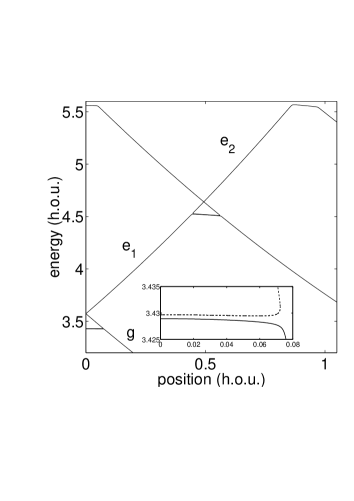
FIG. 1.: The energy of states ground states $g$, and the first two excited states, $e_{1}$ and $e_{2}$ as a function of the barrier position with $h=12$ and $g=0.5$. In the vicinity of the level crossing the upper level is split into three states that form a triangular structure. The ground-excited state splitting is shown inset.

For small $x_{0}$ the energy of the ground state is almost independent of the barrier position. This is because the transfer of atoms through the barrier exactly compensates for the change in potential energy. However, this cannot continue when all the atoms reach one side and the energy becomes strongly position dependent again at the critical displacement, $x_{\rm c}$ ($x_{\rm c}=0.07$ for the parameters in Fig. 1).

At $x_{0}\sim 0.5$ there is a second level crossing where it becomes energetically favourable for the first excited state $e_{1}$ to move from the upper to the lower well. The energy level structure is similar to that at $x_{0}=0$, where it is the ground state population that moves from the upper to the lower well. In both cases, following the eigenenergy curve produces a large change or ‘step’ in the well populations. When considering a moving barrier these steps give rise to a resonance in the tunnelling current. In Section V, we suggest the optimal scheme for observing such tunnelling resonances.

The energy splitting between the ground and lowest excited state is extremely small for $h=12$, see Fig. 1(inset). From an experimental viewpoint, lower barriers resulting in larger energy splittings are more interesting. In Fig. 2 we illustrate how the triangular structures evolve as a function of barrier height with $g=0.5$. The appearance of the loop structure, which coincides with the threshold for self-trapping, occurs at critical height $h=2.916$ (see Section IV). The structure becomes more triangular as $h$ increases.

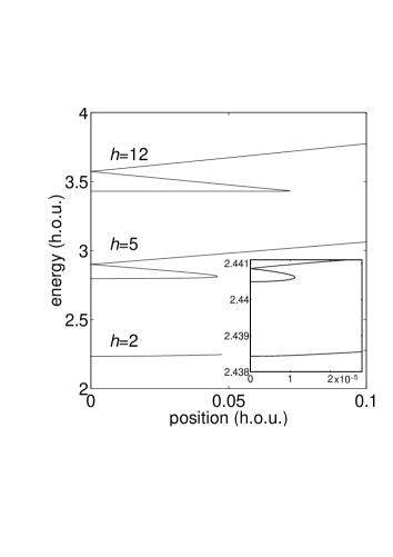
FIG. 2.: The energy of state $e_{1}$ as a function of the barrier position for $g=0.5$ and barrier heights $h=2$, 5, and 12. The energy curves for $h=2.91$ and $h=2.92$ are shown inset. The loop structure appears at $h=2.916$.

In Fig. 3 we show the eigenenergies for $g=0.5$ and $h=4$. In this case, the loop structure appears for the first but not the second excited state. The appearance of a loop structure results in the breakdown of adiabatic following of an eigenenergy curve [14]. In Section V, we will see that this breakdown is associated with a discontinuity in the population difference between the two wells.

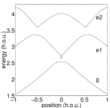
FIG. 3.: The energy of states $g$, $e_{1}$ and $e_{2}$ as a function of the barrier position for $h=4$ and $g=0.5$.

Finally in Fig. 4, we illustrate the effect of increasing the self-interaction parameter to $g=5$. In this case the energy splittings are a significant fraction of the harmonic oscillator energy level spacing and the critical displacement coincides with the position of the crossings between states $e_{1}$ and $e_{2}$. In this regime, the influence of state $e_{2}$ cannot be neglected, and a two-state approximation cannot be used to describe the system.

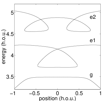
FIG. 4.: The energy of states $g$, $e_{1}$ and $e_{2}$ as a function of the barrier position for a barrier height $h=4$ and $g=5$.

We stress that by solving the Gross-Pitaevskii equation in three dimensions we have obtained eigenenergy curves qualitatively similar to those shown in Figs. 1 to 4.

III Non-linear two-state model

In this section we review the two-state model [4, 6], and apply it to the specific case of a Bose-Einstein condensate in an asymmetric double-well. The wave function, $\psi(t)$, is written as

$$\psi(t) = \phi_{1}(t)\psi_{1}+\phi_{2}(t)\psi_{2}~{},$$ (7)

where the zeroth-order (real) mode functions $\psi_{i}$, $i=1,2$, are eigenfunctions of the time-independent GP equations

$$\mu\psi_{i} = -\textstyle{1\over 2}\nabla^{2}\psi_{i}+V_{i}\psi_{i}+g|\psi_{i}|^{2}\psi_{i}~{}.$$ (8)

The mode potentials $V_{1}$ and $V_{2}$ are single-well potentials displaced to the left and the right of $x=0$, respectively, and satisfy $V_{1}(x)=V_{2}(-x)$ so that $\psi_{1}(x)=\psi_{2}(-x)$. The time-dependent coefficients $\phi_{i}(t)$ can, in turn, be expressed as

$$\phi_{i}(t)=\sqrt{N_{i}(t)}{\rm e}^{i\theta_{i}(t)}~{},$$ (9)

where $N_{i}(t)$ and $\theta_{i}(t)$ are the population and phase of state $i$, with $N_{1}(t)+N_{2}(t)=1$.

Recalling that the two mode functions satisfy $\mbox{$\langle\,{\psi_{1}}\!\mid$}V_{x_{0}=0}\mbox{$\mid\!{\psi_{1}}\,\rangle$}=\mbox{$\langle\,{\psi_{2}}\!\mid$}V_{x_{0}=0}\mbox{$\mid\!{\psi_{2}}\,\rangle$}$ and redefining the zero of energy, we obtain the following non-linear equations of motion for $\phi(t)=(\phi_{1}(t),\phi_{2}(t))^{\rm T}$:

$$i\dot{\phi}(t) = H(\phi(t))\phi(t)~{}.$$ (10)

The non-linear Hamiltonian matrix, $H(\phi(t))$, is given by

$$H(\phi(t))=\frac{1}{2}\left[\begin{array}[]{cc}-\Delta+NE_{\rm C}&-E_{\rm J}\\ -E_{\rm J}&\Delta-NE_{\rm C}\end{array}\right]$$ (11)

where $N=N_{1}-N_{2}$ is the population difference between the left and right sides of the well, and $E_{\rm J}$ and $E_{\rm C}$ are the coupling or Josephson energy and the self-interaction energy, respectively. The self-interaction energy of each mode is

$$E_{\rm C}=g\mbox{$\langle\,{\psi_{1}}\!\mid$}\,|\psi_{1}|^{2}\mbox{$\mid\!{\psi_{1}}\,\rangle$}=g\mbox{$\langle\,{\psi_{2}}\!\mid$}\,|\psi_{2}|^{2}\mbox{$\mid\!{\psi_{2}}\,\rangle$}~{},$$ (12)

and we define the shift in energy of the mode states due to the displacement of the potential barrier to be

$$\textstyle{1\over 2}\Delta = \mbox{$\langle\,{\psi_{1}}\!\mid$}\left(V_{x_{0}=0}-V_{x_{0}}\right)\mbox{$\mid\!{\psi_{1}}\,\rangle$}$$ (13)

$$= \mbox{$\langle\,{\psi_{2}}\!\mid$}\left(V_{x_{0}}-V_{x_{0}=0}\right)\mbox{$\mid\!{\psi_{2}}\,\rangle$}~{}.$$ (14)

If states $\psi_{1}$ and $\psi_{2}$ correspond to the population on the left and right of the barrier, respectively, then linearising yields

$$\textstyle{1\over 2}\Delta \simeq x_{0}\mbox{$\langle\,{\psi_{1}}\!\mid$}\left(\frac{dV_{x_{0}}}{dx_{0}}\right)_{x_{0}=0}\mbox{$\mid\!{\psi_{1}}\,\rangle$}=-\alpha x_{0}~{},$$ (15)

where $\alpha<0$ is the rate of change of the energy with displacement. As will be discussed below, this linear approximation works well when the influence of higher-lying states is negligible. Finally, the coupling energy of the two-modes is

$$\textstyle{1\over 2}E_{\rm J} \simeq -\mbox{$\langle\,{\psi_{1}}\!\mid$}\left(-\textstyle{1\over 2}\nabla^{2}+V_{x_{0}=0}\right)\mbox{$\mid\!{\psi_{2}}\,\rangle$}~{},$$ (16)

where use has been made of the fact that

$$\mbox{$\langle\,{\psi_{1}}\!\mid$}\left(\frac{dV_{x_{0}}}{dx_{0}}\right)_{x_{0}=0}\mbox{$\mid\!{\psi_{2}}\,\rangle$} = 0~{}.$$ (17)

The Hamiltonian, equation (11), is similar to that considered by Wu and Niu in their study of non-linear Landau-Zener tunnelling [14]. In the next section we discuss the eigenstates of $H$ in relation to the numerical solutions discussed in Section II.

IV Eigenenergies of the two-state model

Within the two-state model, one may find the eigenenergies of the system by substituting $\theta_{1}(t)=\theta_{2}(t)=\epsilon t$. The eigenenergies are given by the roots of the quartic equation [14]

$$\epsilon^{4}-E_{\rm C}\epsilon^{3} + \textstyle{1\over 4}(E_{\rm C}^{2}-E_{\rm J}^{2}-\Delta^{2})\epsilon^{2}$$ (18)

$$+ \textstyle{1\over 4}E_{\rm C}E_{\rm J}^{2}\epsilon-\textstyle{1\over 16}E_{\rm C}^{2}E_{\rm J}^{2}=0~{}.$$ (19)

The population difference between the left and right wells is obtained from the eigenenergies via

$$N = \frac{\Delta}{(E_{\rm C}-2\epsilon)}~{}.$$ (20)

An important feature of equation (19) is that there are four real roots when the coefficient of the quadratic term $E_{\rm C}^{2}-E_{\rm J}^{2}-\Delta^{2}$ is positive and only two when it is negative. For a symmetric double-well ($\Delta=0$), the additional roots appear at the critical point where the self-interaction energy satisfies $E_{\rm C}=E_{\rm J}$. For $E_{\rm C}>E_{\rm J}$, the eigenenergies of the stationary states are $\pm E_{\rm J}/2$ and $E_{\rm C}/2$, with the latter being doubly degenerate. The additional roots disappear if the displacement of the barrier is such that $|\Delta|=|2\alpha x_{0}|>\sqrt{E_{\rm C}^{2}-E_{\rm J}^{2}}$.

To test the applicability of the two-state model, we have compared the eigenenergies with those determined from the numerical solution of the GP equation. The energy curves are parametrised by three numbers: the splitting between the two lower levels, which is equal to $E_{\rm J}$; the energy of the self-trapping states, $E_{\rm C}/2$; and an energy gradient, $\alpha$. In a two-state model, $\alpha$ is both the energy gradient of the self-trapping state, and that of the ground state for $x>x_{\rm c}$. For small $g$ and high barriers, such that $E_{\rm C}\gg E_{\rm J}$, $\alpha\sim-E_{\rm C}/2x_{\rm c}$.

Fig. 5 shows a comparison between the exact eigenenergies and the model curves for $h=4$, $g=0.5$. The values of $E_{\rm C}$, $E_{\rm J}$, and $\alpha$ are taken from the exact solutions. The energy gradient is matched to that of the self-trapping states at $x_{0}=0$ ($\alpha=3.187$). This value gives the best agreement when comparing population dynamics (see Section V). However, due to the slight curvature of the eigenenergy curves a smaller value ($\alpha=2.663$) gives a better fit to the triangular structure. The agreement between the two-state model and the exact eigenenergies becomes less good as the influence of higher-lying states increases. For example, the model does not predict the almost flat position dependence of the upper levels in $e_{1}$ for $h=4$, $g=5$, see Fig. 4.

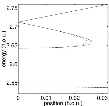
FIG. 5.: Comparison between the exact (solid) and the two-state model (dashed) eigenenergies as a function of the barrier position for $h=4$ and $g=0.5$.

To apply the two-state model one needs to known the value of $E_{\rm J}$, $E_{\rm C}$ and $\alpha$ for any particular barrier height or non-linearity. In Fig. 6 we show how the energy splittings vary with the non-linearity and the barrier height. The critical point, $E_{\rm C}=E_{\rm J}$, appears as either a critical non-linearity or a critical height depending on which parameter is varied. Note that for large non-linearity, the existence of the second excited state, $e_{2}$, effectively puts an upper limit on the value of $E_{\rm C}$.

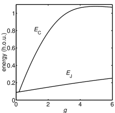
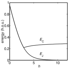
FIG. 6.: The dependence of the self-interaction energy, $E_{\rm C}$, and the Josephson energy, $E_{\rm J}$, on the self-interaction parameter, $g$ (with $h=4$), and the barrier height, $h$ (with $g=0.5$).

In Fig. 7, we show the left-right population difference of the self-trapping state. A population asymmetry appears at the critical point, $E_{\rm C}=E_{\rm J}$, corresponding to the critical barrier height, $h=2.916$ for $g=0.5$. The asymmetry increases with increasing barrier height. As a function of the non-linearity, the self-trapping population first increases, then saturates, and finally decreases at large $g$ due to the influence of $e_{2}$.

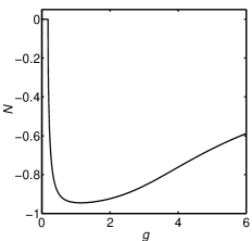
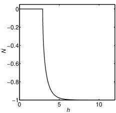
FIG. 7.: The population asymmetry of the self-trapping state as a function of the self-interaction parameter, $g$ (with $h=4$), and the barrier height, $h$ (with $g=0.5$).

V Josephson dynamics

We now apply the eigenstate picture to analyse the population dynamics when the barrier is moved uniformly through the condensate at velocity $v$. The time-dependent GP equation is integrated using a Crank-Nicholson algorithm and the time evolution analysed in terms of transitions between eigenstates. A similar approach was used previously to study vortex nucleation [19].

In Fig. 8 we show both the eigenstate population differences and the calculated evolution of the population difference as the barrier is moved from the canter towards the right at a speed $v=4\times 10^{-5}$ (bold line). This example is similar to the case studied in [9]. The eigenstate population differences appear as straight diagonal lines. For low velocities, the evolution is adiabatic, and the time-dependent solution follows the ground state population difference curve resulting in a dc tunnelling current. Above a critical velocity, there is a transition to a superposition of ground and excited states such that the population difference remains constant, apart from a decaying oscillatory component (see inset). Subsequently, the excited state component encounters a level crossing with higher-lying states which leads to further ‘steps’ in the population difference or resonances in the tunnelling current. For the example of $v=4\times 10^{-5}$ shown in Fig. 8, the speed is just below the critical velocity for the transition from $e_{2}$ to $e_{3}$ leading to a large tunnelling current as the object moves past $x_{0}\sim 0.9$.

A Critical velocity

By defining $\theta(t)=\theta_{1}(t)-\theta_{2}(t)$, and rearranging equations (9–11), one obtains the coupled equations

$$\dot{N}=E_{\rm J}\sqrt{1-N^{2}}\sin\theta~{},$$ (21)

$$\dot{\theta}=\Delta-NE_{\rm C}-\frac{E_{\rm J}N}{\sqrt{1-N^{2}}}\cos\theta~{}.$$ (22)

Differentiating again and substituting for $\dot{N}$ and $\dot{\theta}$ gives

$$\ddot{\theta}=\dot{\Delta}-\frac{E_{\rm J}(E_{\rm C}-N\Delta)}{\sqrt{1-N^{2}}}\sin\theta-\frac{E_{\rm J}^{2}(1+N^{2})}{2(1-N^{2})}\sin 2\theta~{}.$$ (23)

If $N$ is roughly constant, this equation may be re-written as $\ddot{\theta}=-\partial_{\theta}U$, where $U(\theta)$ describes a ‘tilted-washboard’ potential. The critical velocity is determined by setting the minimum gradient of $U(\theta)$ equal to zero. For $N\approx 0$ at $t=0$ and using $\Delta=-2\alpha x_{0}=-2\alpha vt$, one finds

$$v_{\rm c}=-\frac{E_{\rm J}E_{\rm C}}{2\alpha}-\frac{E_{\rm J}^{2}}{4\alpha}~{}.$$ (24)

For $E_{\rm C}\gg E_{\rm J}$, one can use the linear approximation, $\alpha=-E_{\rm C}/2x_{\rm c}$, where $x_{\rm c}$ is the critical displacement, which yields $v_{\rm c}\sim E_{\rm J}x_{\rm c}$. Taking the values from Fig. 1, $E_{\rm J}=7\times 10^{-4}$ and $x_{\rm c}=0.07$, gives $v_{\rm c}\sim 5\times 10^{-5}$. According to equations (21) and (22) the maximum population difference occurs at approximately $v_{\rm c}/\sqrt{2}=3.4\times 10^{-5}$, which is in excellent agreement with the value determined by numerical integration of the GP equation.

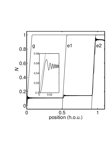
FIG. 8.: The population asymmetries for eigenstates $g$ , $e_{1}$ and $e_{2}$ as a function of the barrier position with $h=12$ and $g=0.5$. The population difference as the barrier is moved from the centre towards the right at speeds of 4$\times 10^{-5}$ is plotted as a thick black line. An expanded view of the evolution for short times is shown inset.

B Asymmetric initial condition

As stated above, the small critical velocity for high barriers (typically less than a micron per second) makes experimental verification challenging. Although higher critical velocities are obtained for lower barriers, the transition between the dc and ac regime becomes less sharp. This problem can be partially circumvented by noting that one can induce larger population changes by starting with an asymmetric well and moving the barrier back through the origin. This is illustrated in Fig. 9 with a lower barrier height, $h=4$. Again for low barrier speeds the population follows the ground state distribution, whereas for faster speeds a transition to an oscillatory current is observed. The critical velocity is a factor of 200 times larger than for $h=12$.

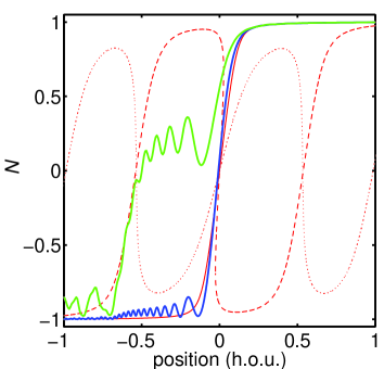
FIG. 9.: The population difference as the barrier is moved from $x_{0}=1$ towards the left at a constant speed of 0.007 (black) and 0.015 (grey) for $h=4$ and $g=0.5$. The corresponding population differences for eigenstates $g$, $e_{1}$, and $e_{2}$ are indicated by the solid, dashed and dotted lines. For $e_{2}$, the gradient of $N$ against $x_{0}$ is always positive, whereas for $e_{1}$ the gradient becomes negative in the vicinity of the level crossing. Recalling that when the barrier is moving the tunnelling current is proportional to this gradient, it follows that the appearance of the triangular structure in $e_{1}$ is associated with an infinite tunnelling current and a complete breakdown of adiabatic evolution.

For $x_{0}<-0.6$ the population difference follows that of the excited state, $e_{1}$, therefore to observe a large population difference, it is important to stop the motion before the barrier reaches $x_{0}\sim-0.4$. This restricts the evolution to short times or low velocities. In Fig. 10 we show the population difference as a function of the barrier speed for both a symmetric and asymmetric starting condition. Fig. 10(a) shows that the two-state model can no longer predict the correct result if the second level crossing is reached, which for $t=30$ occurs when $v>0.015$.

Comparison between Fig. 10(a) and (b) illustrates that a larger population difference and a better demarcation of the critical velocity is obtained by moving the barrier from the edge of the condensate inwards (asymmetric initial condition). The numerical results indicate that the critical velocity for this case is similar to that for the symmetric initial state. However, it is not straightforward to predict the critical velocity for the asymmetric initial condition because the relative importance of the coefficients in equation (23) depends on the instantaneous value of $N(t)$. For $h=12$, $g=0.5$, the critical velocity is a factor of three smaller than for the symmetric initial state.

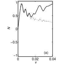
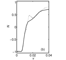
FIG. 10.: Comparison of the Josephson tunnelling with (a) a symmetric and (b) an asymmetric initial condition. The population difference as a function of the barrier speed $v$ obtained from the GP equation (solid line) and the two-state model (dashed line) for $h=4$ and $g=0.5$. In (a) the barrier is moved from the centre outwards for a time $t=30$. For $v>0.015$ the second level crossing is reached leading to a departure between the GP simulation and the prediction of the two-state model. In (b) the barrier is moved from $x_{0}=0.95$ and stopped at $x_{0}=-0.3$. The parameters $E_{\rm C}$, $E_{\rm J}$, and $\alpha$ for the model are taken from the GP eigenenergies.

Finally, we consider the interesting case where the influence of higher-lying states severely limits the applicability of the two-state model. In Fig. 11 we show the population change as a barrier with height $h=4$ is moved through the centre of a condensate with $g=5$. For these parameters the critical velocity is sufficiently high that the level crossing to a higher-lying state is reached before the transition to the ac regime is completed. However, a large population difference for different barrier velocities can still be observed if the motion is halted when the barrier reaches $x_{0}\sim-0.5$.

The large critical velocity, $v_{\rm c}\sim 0.08$, offers the best potential for the experimental observation of Josephson-like tunnelling resonances. For example, taking a typical sodium condensate with a trap frequency of $20$ Hz, the black and grey curves in Fig. 11 correspond to a barrier formed by a blue detuned laser sheet with waist 3 microns, moved by 5 microns in 1.5 s and 1 s, respectively. For these parameters, a model involving higher-lying excited states is essential to give a clear picture of the Josephson population dynamics.

To restate the richness of the double-well system, it is worth noting that as one increases the non-linearity further, the transition from the ground to first excited state corresponds to the formation of a soliton. Consequently by varying only two parameters, the barrier height and the interaction strength, for example using a Feshbach resonance [20], one can explore the complete parameter space between Josephson tunnelling and soliton formation.

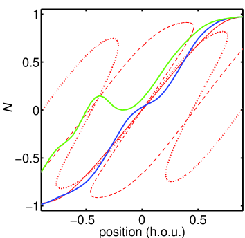
FIG. 11.: The population difference as the barrier is moved from position 0.9 towards the left at speed of 0.05 (black) and 0.08 (grey) for $h=4$ and $g=5$. The corresponding population asymmetries for eigenstates $g$, $e_{1}$, and $e_{2}$ are indicated by the solid, dashed and dotted lines.

VI Conclusions

In summary, we have studied the eigenstates of a dilute Bose-Einstein condensates in an asymmetric double-well potential. We have shown that in the regime of interest for experiments, i.e., with a large non-linearity and a low barrier, a two-state description is insufficient to describe the tunnelling dynamics. By determining the influence of higher-lying states we have demonstrated that large population differences can be observed if the barrier motion is halted before the upper tunnelling resonance is reached.

REFERENCES

- [1] B. P. Anderson and M. A. Kasevich, Science 282, 1686 (1998).
- [2] F. S. Cataliotti, S. Burger, C. Fort, P. Maddaloni, F. Minardi, A. Trombettoni, A. Smerzi, and M. Inguscio, Science 293, 843 (2001).
- [3] M. R. Andrews, C. G. Townsend, H. J. Miesner, D. S., Durfee, D. M. Kurn, and W. Ketterle, Science 275, 637 (1997).
- [4] G. J. Milburn, J. Corney, E. M. Wright, and D. F. Walls, Phys. Rev. A 55, 4318 (1997).
- [5] J. Anglin, Phys. Rev. Lett. 79, 6 (1997).
- [6] A. Smerzi, S. Fantoni, S. Giovanazzi, and S. R. Shenoy, Phys. Rev. Lett. 79, 4950 (1997).
- [7] J. Ruostekoski and D. F. Walls, Phys. Rev. A 58, R50 (1998).
- [8] S. Raghavan, A. Smerzi, S. Fantoni, and S. R. Shenoy, Phys. Rev. A 59, 620 (1999).
- [9] S. Giovanazzi, A. Smerzi, and S. Fantoni, Phys. Rev. Lett. 84, 4521 (2000).
- [10] J. Williams, Phys. Rev. A 64, 013610 (2001).
- [11] F. Meier and W. Zwerger, Phys. Rev. A 64, 033610 (2001).
- [12] A. Vardi and J. R. Anglin, Phys. Rev. Lett. 86, 568 (2001).
- [13] L. Pitaevskii and S. Stringari, Phys. Rev. Lett. 87, 620 (2001).
- [14] B. Wu and Q. Niu, Phys. Rev. A 61, 023402 (2000).
- [15] B. Wu, R. B. Diener, and Q. Niu, cond-mat/0109183.
- [16] D. Diakonov, L. M. Jensen, C. J. Pethick, and H. Smith, cond-mat/0111303.
- [17] T. Winiecki, J. F. McCann, and C. S. Adams, Europhys. Lett. 48, 475 (1999).
- [18] W. H. Press, S. A. Teukolsky, W. T. Vetterling and B. P. Flannary, Numerical recipes in FORTRAN : the art of scientific computing 2nd Ed. CUP, Cambridge, 1992.
- [19] T. Winiecki and C. S. Adams, Europhys. Lett. 52, 257 (2000).
- [20] S. L. Cornish, N. R. Claussen, J. L. Roberts, E. A. Cornell, and C. E. Wieman, Phys. Rev. Lett. 85, 1795 (2000).