Abstract

We compute the largest relaxation times for the totally asymmetric exclusion process (TASEP) with open boundary conditions with a DMRG method. This allows us to reach much larger system sizes than in previous numerical studies. We are then able to show that the phenomenological theory of the domain wall indeed predicts correctly the largest relaxation time for large systems. Besides, we can obtain results even when the domain wall approach breaks down, and show that the KPZ dynamical exponent $z=3/2$ is recovered in the whole maximal current phase.

PACS numbers: 05.40.-a, 05.60.-k, 02.50.Ga

Key words: asymmetric exclusion process, density-matrix renormalization, dynamical exponents

1 Introduction

Several many particle systems are characterized by a steady mass transport. Examples for this kind of systems can be found in biological transport [1] or vehicular traffic [2]. From a theoretical point of view these processes are of particular interest, because they exhibit generic non-equilibrium behavior. Due to the large number of important applications, many microscopic models for particle transport have been suggested in recent years [2, 3, 4].

Among these, the most important microscopic model for non-equilibrium particle transport is the so called asymmetric exclusion process (ASEP) [5, 6]. In this model, particles jump on a one-dimensional lattice, either to the right (with probability $p\;dt$) or to the left (with probability $q\;dt$), if the corresponding sites are empty. The model shows a number of generic effects [7] that are characteristic for non-equilibrium particle transport and maintain for the more specialized variants of the model [8, 9]. At the same time the ASEP is simple enough to obtain several exact results for the system, which is of great importance, because the general theoretical framework of non-equilibrium physics is less developed. Exact results exist, e.g. for the stationary state of the system with periodic [6] and open boundary conditions [10, 11, 12]. The case of open boundary conditions is of special interest because one observes boundary induced phase transitions [7]. In this paper, we restrict ourselves to the totally asymmetric exclusion process (TASEP), that is $q=0$. This case includes the most important phenomena but simplifies considerably the discussion of the model. Open boundary conditions are implemented by two particle reservoirs that are coupled to the chain. The capacities of the reservoirs determine, together with the bulk hopping rates, the actual state of the system.

The complexity of the open system is also reflected in the mathematical structure of the stationary solution. While the steady state of the periodic system is given by a simple product measure [6], it is highly non-trivial for the open system. Nevertheless, it can be calculated and it is possible to obtain several non-trivial quantities, e.g. current- or density fluctuations in the stationary state [10, 11, 12], or large deviation functions [13].

The dynamic properties of the open system are, however, more puzzling. Exact analytical results for the largest relaxation time $\tau$ and the corresponding dynamical exponent $z$ are so far only possible for the periodic chain by applying the Bethe ansatz [14, 15]. For the open chain estimates for $\tau$ can be obtained from a phenomenological approach, that models directly the dynamics of the boundary layer separating the high and low density domains imposed by the particle reservoirs [16]. It has been shown, that this approach gives asymptotically correct results in a certain parameter regime [17]. For finite systems, as well as for general in- and output rates, relaxation times have to be calculated numerically.

This has been done by U. Bilstein and B. Wehefritz [18], and later by M. Dudzińsky and G.M. Schütz [19] who calculated the relaxation times by using exact diagonalization. This method is, however, restricted to very short chains (less than twenty), that are not in the asymptotic limit. In this work we used the density matrix renormalization group (DMRG) technique [20], that enables us to calculate the relaxation times for much larger system sizes, compared to [18, 19]. By treating large chains we have obtained more conclusive results for the dynamical exponent $z$ in the maximal current phase and could also achieve convergence between the exact numerical values of the relaxation times and the estimates of the phenomenological approach.

The paper is organized as follows. In the next section we discuss briefly the relevant physical concepts and the applied numerical techniques. In the third section we show the comparison of the domain wall predictions for finite systems with our results. Section 4 is devoted to the special case of the disorder line $\alpha+\beta=1$. This section is followed by a discussion of the dynamical behavior when approaching the phase boundaries as well as in the maximum current phase.

2 Analytic predictions and the DMRG method for non-equilibrium systems

2.1 The TASEP with open boundary conditions

For self-containedness we will repeat the definition of the model. The TASEP is defined on a one-dimensional lattice with $L$ sites. The boundary sites of the chain are coupled to two particle reservoirs, one reservoir on the left that controls the particle input and a second on the right that governs the output of particles.

We regard the process in continuous time (see [21] for a comparison of the different update procedures), which corresponds to a random sequential update in computer simulations. If a link between sites $i$ and $i+1$ is selected, a particle located at $i$ moves to site $i+1$ if site $i+1$ is empty (for convenience we set the hopping rate to one). In case of choosing the link $(0,1)$ one introduces a particle with probability $\alpha$ if the first site is empty. Finally a particle may leave the system with probability $\beta$, if the link $(L,L+1)$ is chosen.

Each configuration $\sigma$ can be written in terms of boolean lattice gas variables $\sigma_{i}$, i.e. $\sigma_{i}=0(1)$ if the site is empty (occupied). If we introduce an orthonormal basis $|\sigma\rangle=|\sigma_{1},...,\sigma_{L}\rangle$ in the $2^{L}$-dimensional configuration space, we can define the probability vector $|P(t)\rangle$ as $|P(t)\rangle=\sum_{\{\sigma\}}P(\{\sigma\},t)|\sigma\rangle$. The time evolution of $|P(t)\rangle$ is determined by means of the master equation, that can be written as a Schrödinger equation in imaginary time [5, 21]:

$$\frac{\partial}{\partial t}|P(t)\rangle=-{\cal H}\,|P(t)\rangle,$$ (1)

where ${\cal H}$ denotes the stochastic Hamiltonian. The matrix elements of ${\cal H}$ are the rates $w(\sigma\rightarrow\sigma^{\prime})$ for a transition $\sigma\to\sigma^{\prime}$. Explicitly ${\cal H}$ is given by $\langle\sigma|{\cal H}|\sigma^{\prime}\rangle=-w(\sigma^{\prime}\rightarrow\sigma)$ for the off-diagonal elements ($\sigma\neq\sigma^{\prime}$) and by
$\langle\sigma|{\cal H}|\sigma\rangle=\sum_{\{\sigma\}\neq\{\sigma^{\prime}\}}w(\sigma\rightarrow\sigma^{\prime})$ for the diagonal elements.

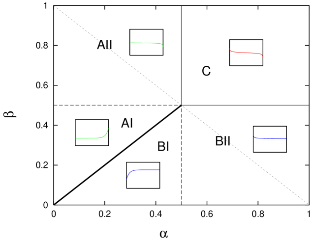
Figure 1: Phase diagram of TASEP with random sequential update, depending on the input rate $\alpha$ and output rate $\beta$. The insets show typical density profiles. Phase transitions are indicated by the solid lines. Along the diagonal dashed line $\alpha+\beta=1$, corresponding to the disorder line of the model, the density profile is flat. Finally, the transitions between the subphases AI / AII (respectively BI / BII) are marked by dashed lines.

The exact stationary solution of the master equation can, for general $\alpha,\beta$, be written as a product of infinite dimensional matrices [11]. This solution allowed to calculate the $\alpha,\beta$ dependence of the stationary quantities, e.g. the average flux. The results are summarized in the phase diagram of the system shown in fig. 1. Three phases can be distinguished by means of a different functional behavior of the flow. In the low density phases AI and AII, i.e. for $\alpha<\beta$, $\alpha<1/2$, the flow $J=J(\alpha)$ is given by $J=\alpha(1-\alpha)$ and analogously in the high density phases BI and BII by $J=\beta(1-\beta)$. If both $\alpha>1/2$ and $\beta>1/2$ (phase C) the capacity of the particle reservoirs exceeds the capacity of the chain. Then the flux is independent of $\alpha$ and $\beta$ and given by $J=1/4$. This phase is called maximal current phase.

Both the high and low density phases are divided into two subphases. In phase AI and BI, the capacities of both reservoirs are below the chain capacity. In phase AII (BII), only the capacity of the exit (entrance) exceeds the chain capacity. This has, e.g. consequences for the asymptotics of the density profile [12], and, a question we address in this article, possibly also for the dynamics of the chain. Another important line is given for $\alpha+\beta=1$. On this one-dimensional line the stationary solution is much simplified, i.e. it is given as product measure.

Now we shall summarize known results for the relaxation times. For the periodic system, exact results for the energy-gap, i.e. the inverse of the largest relaxation time $\tau_{1}$, have been obtained by Bethe-ansatz techniques [14, 15]. The largest relaxation time scales for any density of the system asymptotically as $\tau_{1}\sim L^{z}$, where $z=3/2$.

As translational invariance is lost in the open system, the technique does not apply. Besides, the dynamics is profoundly modified by the presence of the two particle reservoirs, which impose the coexistence of two domains into the system. In case of the phases $AI,BI$, it is known that the two domains imposed by the reservoirs have a simple factorized structure. In this parameter regime the so-called domain wall (DW) theory can be applied [16]. The DW theory uses a coarse grained description of the dynamics of the process: Each particle reservoir that is coupled to the chain imposes independently a domain of a given constant density $\rho_{L}$ and $\rho_{R}$. The two domains are separated by a localized domain wall, which performs a biased random walk. The bias is due to the different capacity of the two reservoirs and can be calculated simply by using the conservation of mass. In a finite system the position of the domain wall is confined between two reflecting walls. The description of the process allows to calculate the stationary as well as the fully time dependent probability distribution of the domain wall positions [19]. Then, it is in particular possible to estimate the largest relaxation times of the system, that are given by

$$\tau_{n}=\left[D^{+}+D^{-}-2\sqrt{D^{+}D^{-}}\cos(\pi n/(L+1))\right]^{-1}\qquad n=1,2,\dots$$ (2)

with

$$D^{+}={\beta(1-\beta)\over 1-\alpha-\beta};\;\;\;D^{-}={\alpha(1-\alpha)\over 1-\alpha-\beta}.$$ (3)

These results are valid for $\alpha,\beta<0.5$. The remaining parameter space has to be explored numerically.

2.2 The DMRG method for stochastic models

In the previous section we have shown that the master equation can be rewritten as a Schrödinger equation in imaginary time. Now, in order to calculate the longest relaxation time of the system, one has to calculate the two lowest eigenvalues of eq. (1) (the first eigenvalue is trivially zero, with an eigenvector corresponding to the stationary state). The eigenvalue calculations have to be done with very efficient diagonalization methods, in order to reach sufficiently large system sizes. This is possible by applying the DMRG method [22].

This method was first developed to study the properties of strongly correlated electrons [20]. It has recently been generalized in order to treat stochastic many particle systems [23, 24].

The idea of the DMRG is the following. One starts with a small system (here 12 sites) that can be diagonalized with standard numerical methods. Then one performs a large number of renormalization cycles in order to increase the system size. At each renormalization cycle, first the system is enlarged by adding 2 sites in the bulk of the system, i.e. in a place where it is less likely that the eigenmodes will be perturbed. The largest eigenvalues of the corresponding enlarged Hamiltonian are computed. These eigenvectors are used in order to construct the density matrix of the system, which will be used in the next stage. Second, in order to avoid an exponential growth of the hamiltonian, a projection onto the “most important” modes has to be done. It has been shown that the best choice is to keep the $m$ leading eigenvectors of the density matrix [20]. The parameter $m$ has to be chosen small enough in order to allow a fast calculation of the eigenvectors, but large enough in order to obtain a high numerical precision. The error due to each truncation is well controlled [22].

Although no fundamental differences between the DMRG method for stochastic and quantum mechanical systems exist, one has to make a certain effort in order to overcome the numerical difficulties. This has been done following the suggestions of ref. [23, 24]. We now discuss some details of our implementation.

The main difference between the quantum mechanical and stochastic problem is that the stochastic hamiltonian is not hermitian. Therefore, the calculation of the eigenvectors of the hamiltonian required at each renormalization step cannot be done by standard diagonalization techniques (as the basic Lánczos or Davidsson algorithms) but one has to apply, e.g. the Arnoldi method or Lánczos for non-symmetric matrices. These methods are quite efficient but, compared to their analogues for symmetric matrices, less stable [25]. We use the Arnoldi method, that turned out to be numerically more stable than the Lánczos method for non-symmetric matrices. Nevertheless the method is numerically well controlled, because the accuracy of the calculated eigenvector can be obtained via the residual norm, i.e. we check that it is indeed an eigenvector. Actually, we have used the Arnoldi method in an iterative way, where the initial guess is the result of the previous Arnoldi run, until the desired precision is reached.

Apart from being non-hermitian, there is another difference between stochastic and quantum mechanical problems. It is well known that the lowest eigenvalue of stochastic hamiltonians is always zero, corresponding to the existence of a stationary state, and that the corresponding left eigenvector $|0_{l}\rangle$ has all its coordinates equal to 1. Therefore the first task will be to calculate the right eigenvector $|0_{r}\rangle$. As we are interested in the asymptotic dynamics of the system, we have to calculate the energy gap G(L) as well, i.e. the next smallest eigenvalue and the corresponding left and right eigenvectors $|1_{l}\rangle$ and $|1_{r}\rangle$. Then the longest relaxation time $\tau=\tau_{1}$ will be given by

$$\tau=G(L)^{-1}.$$ (4)

After the calculation of these eigenmodes, one has to eliminate the least important degrees of freedom of the system, in order to keep the system at a manageable size. It has been shown that the relevant degrees of freedom are the eigenmodes associated to the largest eigenvalues of the density matrix $\hat{\rho}$. The latter is defined depending on how many eigenmodes we need to calculate. Here, for the calculation of the gap, we take

$$\hat{\rho}={1\over 2}\hat{Tr}\left\{|0_{l}\rangle\langle 0_{l}|+|0_{r}\rangle\langle 0_{r}|+|1_{l}\rangle\langle 1_{l}|+|1_{r}\rangle\langle 1_{r}|\right\}.$$ (5)

Note that it is always possible to construct a symmetric form for the density matrix. Therefore, standard algorithms can be applied in order to calculate all eigenvalues and eigenvectors of $\hat{\rho}$ as for quantum systems.

Another trick that allowed to gain accuracy on the gap calculation is to compute first the right eigenmode $|0_{r}\rangle$ for the fundamental state (the left is known), and then to define a new hamiltonian

$$H^{\prime}(\Delta)=H+\Delta|0_{r}\rangle\langle 0_{l}|.$$ (6)

This hamiltonian $H^{\prime}$ has, apart from the groundstate, the same spectrum as the original hamiltonian $H$. The gap is now given by the fundamental state of $H^{\prime}$ [24].

Note that one requirement of the DMRG method is that the requested eigenvalue is well separated from the next one. This may not be true when the system size increases, and then the calculation becomes instable. The system size limitations come from these instabilities rather than from runtime or memory requirements. So, the DMRG method either gives very accurate results for the eigenvalues, or does not converge at all.

Finally we want to mention another particularity of the system. As rules are different at each end of the system (input or output), we cannot use the left/right symmetry of the system as people do for closed systems, and the left and right parts of the system have to be computed alternatively.

3 Test of the Domain Wall Theory at Small System Sizes

The comparison between DW predictions and the exact analytical for the stationary state shows that they agree in the limit of large system sizes and $\alpha,\beta<1/2$ [17]. For finite systems, however, the coarse grained picture slightly deviates from the exact results.

In case of the dynamical properties, so far no exact analytical results exist. Therefore the DW predictions have to be checked with numerical methods.

In a previous work, we have compared time-dependent density profiles in a non-stationary regime, and found good agreement with the domain wall predictions [26]. Here, we calculate explicitly the relaxation times of the process, in order to compare with the predictions of the DW method. The same has been done already by using the non-symmetric Arnoldi method [18, 19], but the system sizes that one can treat by the non-symmetric Arnoldi method are too small ($L\leq 16$ in [19]) in order to obtain convergence with the DW predictions. Our aim is to improve this convergence thanks to the ability of DMRG to treat larger systems.

First we consider cases with both $\alpha$ and $\beta<1/2$, where the domain wall theory is expected to work well, though this was not fully verified by the exact numerical calculation, due to size limitations. Fig. 2 shows the comparison of the inverse relaxation time with the domain wall predictions in the high density phase ($\alpha=0.2$, $\beta=0.1$). For comparison we also included the result for $L=16$ obtained in [19], which perfectly coincides with the DMRG calculations. Obviously the theoretical predictions and the numerical results are in good agreement, if the length of the chain reaches thirty sites.

Figure 2: Gap as a function of the system size, for $\alpha=0.2$ and $\beta=0.1$. The solid line indicates the domain wall prediction, while symbols represent the DMRG results. The circle was obtained in [19] for L=16. Error bars for the DMRG results are not given, as they are much smaller than the size of the symbols. The inset shows in a log-log plot the difference between the two curves.

For $\alpha=0.4$ and $\beta=0.2$, the DW predictions for small system sizes are slightly less accurate, as shown in figure 3. This could be expected, as the density difference between the two domains $\Delta\rho=1-\beta-\alpha$ is smaller and therefore the width of the shock larger than in the previous case. If, however, the shock touches the boundaries the approximation of microscopic states by $\Theta$-functions is less appropriate.

Figure 3: Gap as a function of the system size, for $\alpha=0.4$ and $\beta=0.2$. The solid line indicates the domain wall prediction, while symbols represent the DMRG results. The insets shows in a log-log plot the difference between the two curves.

For $\alpha$ or $\beta$ larger than 0.5, the coexistence is not between a high- and low-density domain, but, e.g. for $\alpha>1/2$, between a maximal current and high-density domain. This case is much more complicated than the coexistence of domains in the phase $AI$ or $BI$. It is known from the exact results, that long ranged correlations exist in the maximal current regime, which implies that the maximal current domain has no simple structure, and cannot be easily described.

A naive attempt to describe the maximal current domain, which uses the fact that the flux is a constant $J=1/4$ and would lead to exponentially decaying density profiles, is to build the density profile iteratively from the boundary with a mean field formula like $j=\rho_{i}(1-\rho_{i+1})$. But this yields a wrong density profile. It was also suggested [19] to use the exact results of the density profile. However, this approach has intrinsic shortcomings. First the DW is no longer self-contained and, second, it is no longer possible to specify the relaxation times in a closed form, because the hopping rates of the random walk are now site-dependent. But above all, the description of the system states as the juxtaposition of two phases with an independent boundary layer between them breaks down. Indeed, the wall dynamics is coupled to the whole structure of the maximal current phase, due to the long ranged correlations.

So we explore this parameter regime guided by two questions: $(i)$ Do we obtain a finite relaxation time in the phases $AII/BII$ in the limit of large system sizes? $(ii)$ And, if it is the case, is it possible to model the maximum current phase as a flat domain with an effective density $\rho_{eff}$?

First we checked the domain wall predictions close to the transition line at $\alpha=0.5$, i.e. for $\alpha=0.51$ and $0.55$ (see figure 4). In this parameter regime one already has long ranged correlations in the maximal current domain, but at the same time the magnitude of the deviations from a flat domain is rather small. Our results indicate, that within this parameter regime the DW formulas (2-3) still lead to satisfying results for quite large system sizes. On the other hand, the DW prediction with $\alpha=1/2$, which was conjectured at first to be the proper one for any $\alpha>1/2$ [19], clearly underestimates the gap for any system size.

For larger values of $\alpha$ (e.g. $\alpha=0.65$ in figure 4), the algebraic corrections of the density profile become non-negligible. Equations (2-3) do not give anymore a good estimate.

Figure 4: Gap as a function of the system size, for $\alpha=0.51$, $0.55$, and $0.65$, and $\beta=0.3$. The solid lines indicate the domain wall prediction, while the symbols represent the DMRG results. The domain wall prediction for $\alpha=0.65$ is the upper curve. The dotted line gives the domain wall prediction calculated for $\alpha=1/2$. The DMRG results $y_{\alpha}(L)$ were interpolated using an algebraic fit function $f(L)=aL^{b}+c$. The inset shows $\log[f(L)-c]$ as a function of $\log L$ (symbols) in comparison with $\log[y_{\alpha}(L)-c]$ (solid lines).

Next, we checked whether our results are compatible with a finite relaxation time in the limit $L\to\infty$. Therefore we interpolated our results for $G(L)$ using the functional form $f(L)=aL^{b}+c$. We find a very good agreement between the fits and our numerical data, with a finite value of $c$ (see the inset of fig. 4), which indicates that the relaxation times remain finite. Our estimates for the relaxation times are $\tau(\infty)=116.(6)$ for $\alpha=0.51$, $\tau(\infty)=101.(7)$ for $\alpha=0.55$, and $\tau(\infty)=96.(1)$ for $\alpha=0.65$.

A finite relaxation time for $L\to\infty$ implies at the same time, that the dynamical exponent vanishes. This can be checked systematically by calculating the size dependent dynamical exponent given as:

$$z(L)=-\frac{\ln\left[G(L+2)\right]-\ln\left[G(L)\right]}{\ln(L+2)-\ln(L)}.$$ (7)

Figure 5: Size dependent dynamical exponents for different values of $\alpha$ ($\beta=0.3$). The results are compatible with $z(\infty)=0$.

Figure 5 shows that our results are compatible with $z=0$ for all values of $\alpha$ we took into account. So these results for $\alpha>0.5$ further support that the relaxation times are finite within these subphases.

Now, one can simply take the values $\tau(\infty)$ in order to calculate an effective density of the maximal current domain. This procedure leads to DW predictions for small systems, which do not agree very well with our numerical findings. We thus believe that the non-trivial structure of the maximal current domain must be considered in modeling the domain wall motion.

4 Disorder line

For general $\alpha,\beta$ it has been shown that the stationary weights are given as products of infinite dimensional matrices. Nevertheless a one-dimensional line in the parameter space exist, i.e. $\alpha+\beta=1$, where the stationary weights are simple products as for the periodic systems. These product states are in analogy with disordered states of quantum spin models. At the disordered line the system is homogeneous, i.e. one can not identify two different domains. This implies that the relaxation at this particular line is not governed by the motion of the domain wall.

Then it is an open question to know whether dynamical properties are changed on this line and how the dynamical properties compare to the periodic system. For the periodic system, Bethe ansatz predicts the dynamical exponent $z=3/2$ [14, 15]. Besides, the first non-zero eigenvalue has an imaginary part except for the density $1/2$. The divergent relaxation times of the periodic system are, however, related to its translational invariance [27].

By contrast, for the open system it is expected that the relaxation times are finite if $\alpha\neq 0.5$, because the density fluctuations spread with a nonzero drift velocity [7].

First, we have applied the DMRG method to the special point $\alpha=\beta=0.5$, where the drift velocity of an excess density vanishes.

Figure 6: Dynamical exponent $z$ as a function of the system size, for $\alpha=\beta=0.5$.

Fig. 6 shows that our numerical results for $z(L)$, obtained up to $L=244$, agree with the exponent $z=3/2$ predicted for the periodic system.

Figure 7: Dynamical exponent $z$ as a function of the system size, along the disorder line. The curves from bottom to top correspond to $\alpha=0.1$, $0.2$, $0.3$, $0.35$, $0.4$, and $0.45$. Error bars are of the same order as the line thickness.

We have also explored the remaining part of the disorder line. We present our simulation results in fig. 7. They seem to exclude the case $z=3/2$, and indicate that the relaxation time would be finite in the large $L$ limit ($z(\infty)=0$).

Although these results are consistent with the expected relaxation behavior, we cannot exclude that a branch corresponding to complex eigenvalues could cross our solution when $L$ becomes large. The DMRG method does not allow to distinguish whether the numerical instabilities are due to the intersection or the convergence of two eigenvalue branches.

Nevertheless, we state that our numerical results are in accordance with a finite relaxation time and, therefore, consistent with the physical picture which was presented in [7]. Further support for this scenario comes from its position in the phase diagram. The disordered line touches a phase boundary only in a single point, i.e. for $\alpha=\beta=1/2$. All other points of the disordered line are located inside a phase where the relaxation times of the system are finite. Therefore, it would be rather counter-intuitive to observe a diverging relaxation time for these parameters.

5 Phase transitions and the maximal current phase

If the capacity of both particle reservoirs exceeds the capacity of the chain, the maximal current phase is realized. In the maximal current phase both localization lengths are infinite. This divergence of length scales leads, e.g. to an algebraic slope of the density profiles.

In this phase, previous numerical calculations by Bilstein et al [18] for $L\leq 20$ extrapolated to large systems seemed to indicate an exponent $3/2$ in the whole maximal current phase.

Figure 8: Dynamical exponent $z$ as a function of the system size, for $\beta=0.8$. The left figure presents results obtained in the AII phase, where the maximal current phase coexist with a high density phase. For $\alpha=0.5$, we are exactly on the 2nd order transition line. The right figure shows results within the maximal current phase.

We have computed the dynamical exponent in various points in the maximal current phase. Results are presented in figure 8, for a constant $\beta=0.8$, $\alpha$ being varied through the second order transition ($\alpha=0.5$) and inside the maximal current phase (we have checked that of course, results are the same when $\alpha$ and $\beta$ are interchanged). We clearly see a transition when the maximal current phase is entered. On the transition line $\alpha=0.5$, we recover $z=3/2$ in the large system size limit. Besides, from our numerical results, the infinite size dynamical exponent seems to be equal to $3/2$ in the whole maximal current phase, confirming the extrapolation in [18].

6 Conclusion

The use of a DMRG approach to compute the largest relaxation time in the TASEP model has allowed to give new strong evidence of the validity of the domain wall picture when reservoirs control the flow.

For $\alpha$ or $\beta$ larger than 1/2, the capacity of one of the reservoirs becomes larger than the chain capacity, and one of the coexisting domains is then a maximal current phase. Our numerical results indicate that the relaxation times $\tau(\infty)$ are finite for $L\to\infty$ as in the phases $AI/BI$. As the bulk density in a maximal current phase is $1/2$ independently of the boundaries, one could have expected that the relaxation time $\tau(\infty)$ would be independent of the most efficient reservoir (i.e. independent of $\beta$ in AII and $\alpha$ in BII). This is not the case, as boundary layers in the maximal current domain decay only algebraically, and lead to a site-dependence of the density. Besides, strong correlations that cannot be easily characterized exist in this phase. This means that the maximal current phase cannot be modeled as a flat domain with density $1/2$.

But even if we model the maximal current domain as a domain of a constant effective density $\rho_{eff}$, which leads to the estimated value of $\tau(\infty)$, we observe large deviations between DW predictions and relaxation times for finite system sizes - again due to the non trivial structure of the maximal current domain. The DW predictions would probably be much improved if one considers site dependent hopping rates, but they are difficult to obtain since the structure of an isolated maximal current domain is not known.

Anyhow, as in phase AI and BI, the domain wall theory still offers a simple explanation for a finite relaxation time of the system in phases AII and BII.

On the disorder line, this picture cannot be applied, as no domain wall can be identified anymore, and a qualitatively different dynamical behavior cannot be excluded. However, though a wall cannot be defined anymore, we could still trace the dynamics of the density fluctuations by introducing a second class particle. The second class particle performs a biased motion to one of the boundaries for any density different from $1/2$. Therefore one expects that the density fluctuations are also driven out of the system with a finite velocity, which should lead to finite relaxation times, if $\alpha\neq 1/2$ [7].

Contrary, in the periodic system, which has the same simple structure of stationary state, the relaxation times diverge as $L\sim L^{3/2}$ for arbitrary densities. The divergent relaxation times have been related to the translational invariance of the periodic system [27] and are, therefore, not expected in case of the open system, except if $\alpha=\beta=1/2$.

Indeed, our numerical results support this scenario. Besides, we have shown that the dynamical exponent $z=3/2$ is also recovered in the whole maximal current phase, for which no theoretical prediction exists.

So we could summarize the expected behavior of the relaxation time as follows :

(i) In the whole phases AI, AII, BI, and BII, except on the transition line $\alpha=\beta$, our results are consistent with a converging relaxation time. Its limit value as $L\rightarrow\infty$ is known from the DW theory in AI and BI.

(ii) On the line $\alpha=\beta$, and in the whole maximal current phase, the relaxation time diverges when $L\rightarrow\infty$. The associated dynamical exponent $z$ is $2$ on the line $\alpha=\beta$ and $3/2$ in the maximal current phase and at the point $\alpha=\beta=1/2$.

Further improvement could be obtained from the use of Finite Size algorithm for DMRG (FSM), as described by Carlon et al [23], in order to gain some precision on our calculations - and thus to reach larger system sizes - in the whole phase diagram, and especially near critical lines.

It would also be interesting to apply the DMRG method to other models, which have a non-trivial but not necessarily site dependent domain structure, in order to check whether the DW theory still describes correctly the relaxation behavior of the system.

Acknowledgments: We acknowledge fruitful discussions with B. Derrida, J. Krug and E. Carlon, and precious remarks from G. Schütz. L.S. acknowledges kind hospitality at the L.P.S. and financial support by C.N.R.S.

References

- [1] J.T. MacDonald and J.H. Gibbs, Biopolymers 7, 707 (1969)
- [2] D. Chowdhury, L. Santen, and A. Schadschneider, Phys. Rep. 329, 199 (2000)
- [3] V. Privman (ed.), Nonequilibrium Statistical Dynamics in One Dimension, (Cambridge University Press, Cambridge, 1997)
- [4] J. Marro, R. Dickman, Nonequilibrium Phase Transitions in Lattice Models, (Cambridge University Press, Cambridge, 1999)
- [5] G.M. Schütz, in: Phase Transitions and Critical Phenomena, Vol. 19, eds. C. Domb and J.L. Lebowitz (Academic Press, New York, 2000)
- [6] H. Spohn, Large Scale Dynamics of Interacting Particles, (Springer, Berlin, 1991)
- [7] J. Krug, Phys. Rev. Lett. 67, 1882 (1991)
- [8] V. Popkov and G.M. Schütz, Europhys. Lett. 48, 257 (1999)
- [9] V. Popkov, L. Santen, A. Schadschneider, and G.M. Schütz, J. Phys. A 34, L45 (2001)
- [10] B. Derrida , E. Domany, and D. Mukamel, J. Stat. Phys. 69, 667 (1992)
- [11] B. Derrida, M.R. Evans, V. Hakim, and V. Pasquier, J. Phys. A 26, 1493 (1993)
- [12] G.M. Schütz and E. Domany, J. Stat. Phys. 72, 277 (1993)
- [13] B. Derrida, J.L. Lebowitz and E.R. Speer, Phys. Rev. Lett. 87, 150601 (2001); B. Derrida, J.L. Lebowitz and E.R. Speer, cond-mat/0205353.
- [14] L.-H. Gwa and H. Spohn, Phys. Rev. A 46, 844 (1992)
- [15] D. Kim, Phys. Rev. E, 52 3512 (1995)
- [16] A.B. Kolomeisky, G.M. Schütz, E.B. Kolomeisky, and J.P. Straley, J. Phys. A 31, 6911 (1998)
- [17] V. Belitzky and G.M. Schütz, to be published
- [18] U. Bilstein and B. Wehefritz, J. Phys. A 30, 4925 (1997)
- [19] M. Dudzinski and G.M. Schütz, J. Phys. A 33, 8351 (2000)
- [20] S.R. White, Phys. Rev. Lett. 69, 2863 (1992)
- [21] N. Rajewsky, L. Santen, A. Schadschneider, and M. Schreckenberg, J. Stat. Phys. 92, 151 (1998)
- [22] S.R. White, Phys. Rep. 301, 187 (1998)
- [23] E. Carlon, M. Henkel, and U. Schollwöck, Eur. Phys. J. B 12, 99 (1999)
- [24] E. Carlon, M. Henkel, and U. Schollwöck, Phys. Rev. E 63, 036101-1 (2001)
- [25] G.H. Golub and C.F. van Loan, Matrix Computations, 3rd edition (Baltimore, 1996)
- [26] L. Santen, and C. Appert, J. Stat. Phys. 106, 187 (2002)
- [27] H. v. Beijeren, J. Stat. Phys. 63, 47 (1991)