Detecting the Kondo screening cloud in conductance measurements on quantum dots

Abstract

The observation of the Kondo effect in quantum dots has provided new opportunities to finally observe the controversial Kondo screening cloud. We study how screening cloud effects appear in the conductance through a quantum wire containing a quantum dot when the length of the wire is comparable to the size of the screening cloud.

One of the most remarkable triumphs of recent progress in nanoelectronics has been the observation of the Kondo effect in a single semi-conductor quantum dot.dot ; Cronenwett ; Wiel The quantum dot is formed in a semiconductor heterolayer by applying voltages which confine electrons to an island of size a fraction of a micron. When the tunneling amplitude to the dot from the external leads is sufficiently small, the number of electrons on the dot becomes quite well-defined leading to the Coulomb blockade effect on the conductance. When the number of electrons on the dot is odd, it can behave as an $S=1/2$ magnetic impurity and the transmission and back-scattering of electrons is described by a magnetic exchange interaction between this impurity and the conduction electrons. The Kondo effect is a renormalization of this exchange interaction to large values at low temperature, $T<T_{K}$, where $T_{K}$ is the Kondo temperature, leading ultimately to ideal $2e^{2}/h$ conductance. This Kondo effect results from the formation of a spin singlet between the impurity spin and a conduction electron in a very extended wave-function, known as the screening cloud. The size of this screening cloud is of order $\xi_{K}\approx v_{F}/T_{K}$ where $v_{F}$ is the Fermi velocity and is of order 1 micron.

Some of these semiconductor devices have the quantum dot embedded in a quantum wire of width comparable to the dot dimension and length of order 1 micron. The ends of the wire must be connected, ultimately, to three-dimensional leads in order to perform conductance measurements. In this situation, the Kondo screening cloud may fill the entire quantum wire and even extend beyond it into the macroscopic leads. One might expect some modification, perhaps suppression, of the Kondo effect to occur if the quantum wire is shorter than the screening cloud. If so, this could provide an ultimate limitation on miniaturization of some nanoelectronic devices.

We have recently investigated this effect in a somewhat different situation where the quantum wire containing the quantum dot is made into a closed ring. Unfortunately, it is then impossible to perform a standard conductance measurement. However, the persistent current induced by a magnetic flux is also sensitive to screening cloud effects and is drastically reduced when the circumference of the ring becomes smaller than $\xi_{K}$.Affleck While this demonstrates the importance of screening cloud effects, such a persistent current measurement would be a difficult experiment. Thus we turn our attention here to an experimentally easier but theoretically more challenging device: a quantum dot embedded in a quantum wire which is in turn connected to external leads by weak tunnel junctions. We assume that a gate voltage can be applied to the dot and also to the quantum wires. We note that a related device has been proposed recently by Thimm et al. Thimm where a Kondo impurity was equally coupled to all energy levels of a finite size box. The energy level spacing was assumed constant and of $O(1/V)$ where $V$ is the volume of the (3 dimensional) box. These two aspects differ considerably from the geometry studied here, since the electrons need to pass through the dot to contribute to the conductance. Moreover, the Non Crossing Approximation used in [Thimm, ] might be questionable in such geometry where several new energy scales emerge compared to the usual Kondo model.

Figure 1: Schematic representation of the device under consideration. $\epsilon_{D}$ and $\epsilon_{W}$ control respectively the dot and wire gate voltage.

A simplified one-dimensional tight-binding model which describes our device is indicated in Fig. 1 and has the Hamiltonian:

$$H=H_{L}+H_{W}+H_{D}+H_{LW}+H_{WD},$$ (1)

where $L$, $W$ and $D$ stand for leads, wires and dot respectively. Here:

$$H_{L} = -t\left[\sum_{j=-\infty}^{-L-2}+\sum_{j=L+1}^{\infty}\right](c^{\dagger}_{j}c_{j+1}+h.c.)$$

$$H_{W} = -t\left[\sum_{j=-L}^{-2}+\sum_{j=1}^{L-1}\right](c^{\dagger}_{j}c_{j+1}+h.c.)$$ (2)

$$+\epsilon_{W}\left[\sum_{-L}^{-1}+\sum_{1}^{L}\right]n_{j}$$

$$H_{D} = \epsilon_{D}n_{0}+Un_{0\uparrow}n_{0\downarrow}$$

$$H_{LW} = -t_{LW}(c^{\dagger}_{-L-1}c_{-L}+c^{\dagger}_{L}c_{L+1}+h.c.)$$

$$H_{WD} = -t_{WD}(c^{\dagger}_{-1}c_{0}+c^{\dagger}_{0}c_{1}+h.c.)$$

Here $n_{j\sigma}\equiv c^{\dagger}_{j\sigma}c_{j\sigma}$ and $n_{j}\equiv n_{j\uparrow}+n_{j\downarrow}$. Effects being left out of our simple model include other impurities in the quantum wires and the presence of several channels. (The quantum wires studied in [Wiel, ] apparently contained about 10 channels.) We also ignore electron-electron interactions in the wires and leads, only keeping them in the dot.

We will assume that the system is in the strong Coulomb blockade regime, so that $t_{WD}<<-\epsilon_{D}$, $U+\epsilon_{D}$, where $\epsilon_{D}<0$. Then we may eliminate the empty and doubly occupied states of the dot, so that $H_{D}+H_{WD}$ gets replaced by a Kondo interaction plus a potential scattering term:

$$H_{WD}+H_{D}\to H_{K} = J(c^{\dagger}_{-1}+c^{\dagger}_{1}){\vec{\sigma}\over 2}(c_{-1}+c_{1})\cdot\vec{S}$$ (3)

$$+ V(c^{\dagger}_{-1}+c^{\dagger}_{1})(c_{-1}+c_{1})$$

with $J=2t_{WD}^{2}\left[{1\over-\epsilon_{D}}+{1\over U+\epsilon_{D}}\right]$, $V={t_{WD}^{2}\over 2}\left[{1\over-\epsilon_{D}}-{1\over U+\epsilon_{D}}\right]$. Here $\vec{S}$ is the spin operator for the quantum dot. We assume that the Kondo interaction and the lead-wire tunneling are weak, $J,t_{LW}<<t$.

In the case of a closed ring, we showed earlier that the renormalization of the Kondo coupling is cut off, even at low temperatures, by the ring circumference.Affleck In the present situation, this renormalization would be cut off by the finite length, $L$, of the quantum wires, if $t_{LW}=0$. Essentially, if the Kondo cloud doesn’t have sufficient room to form, then the growth of the Kondo coupling constant is cut off. The effective Kondo coupling at the length scale $L$ becomes of O(1) when $L\approx\xi_{K}$.

What is less obvious, is what happens for small but finite $t_{LW}$. Then, even if $L<<\xi_{K}$, the Kondo cloud can still form by leaking into the leads. The growth of the Kondo coupling is not cut off by the finite size of the wire. Nonetheless, we might expect some noticeable effects to occur when $L$ is reduced to a value of $O(\xi_{K})$, associated with the screening cloud beginning to leak into the leads. It is these effects which we wish to study in the present paper.

It is instructive to begin with a calculation of the conductance that treats $t_{LW}$ exactly but treats $J$ in lowest non-vanishing order of perturbation theory. We expect this to be valid at sufficiently high $T$ when the renormalized coupling is sufficiently small. To do this calculation, we first diagonalize the Hamiltonian at $J=0$. i.e. we diagonalize $H_{0}\equiv H_{L}+H_{W}+H_{LW}$. For non-zero $t_{LW}$, the spectrum of $H_{0}$ is continuous. In order to study the Kondo interaction in perturbation theory, it is useful to express $c_{1}+c_{-1}$ in terms of the even eigenstates, $c_{\epsilon}$ of $H_{0}-\mu N_{e}$: ${(c_{1}+c_{-1})\over\sqrt{2}}=\int_{-2t-\mu}^{2t-\mu}d\epsilon f(\epsilon)c_{\epsilon}.$ We normalize $c_{\epsilon}$ so that $\{c_{\epsilon},c^{\dagger}_{\epsilon{{}^{\prime}}}\}=\delta(\epsilon-\epsilon{{}^{\prime}})$. Then $f(\epsilon)$ obeys the normalization condition $\int_{-2t-\mu}^{2t-\mu}d\epsilon|f(\epsilon)|^{2}=1.$ For small $t_{LW}$, this “local density of states”, $\rho(\epsilon)\equiv|f(\epsilon)|^{2},$ has sharp peaks at the energies $\epsilon_{n}=\epsilon_{W}-\mu-2t\cos[k_{n}],$ where the momenta $k_{n}\approx\pi n/L+O(t_{WL}^{2}/Lt^{2})$. The separation between these peaks, near zero energy is $\Delta_{n}\approx\pi v_{F}/L$. The width of these peaks is approximately $\delta_{n}=(2t_{LW}^{2}\sin^{3}(k_{n})\eta_{n,W}/tL$ with:

$\eta_{n,W}=\sqrt{1+\epsilon_{W}\cos k_{n}/(t\sin^{2}k_{n})-\epsilon_{W}^{2}/(4t^{2}\sin^{2}k_{n})}$.

We see that the ratio of width to separation is of order:

$$\delta_{n}/\Delta_{n}\approx{t^{2}_{LW}\over t^{2}}{\sin^{2}k_{n}\over\pi}\eta_{n,W}.$$ (4)

We will assume that this quantity is $<<1$. The full Hamiltonian may be written in this basis as:

$$H-\mu N_{e}=\int_{-2t-\mu}^{2t-\mu}d\epsilon\epsilon c^{\dagger}_{\epsilon}c_{\epsilon}$$

$$+\int d\epsilon d\epsilon{{}^{\prime}}f^{*}(\epsilon)f(\epsilon{{}^{\prime}})\left(2Jc^{\dagger}_{\epsilon}{\vec{\sigma}\over 2}c_{\epsilon{{}^{\prime}}}\cdot\vec{S}+2Vc^{\dagger}_{\epsilon}c_{\epsilon{{}^{\prime}}}\right)$$ (5)

The linear conductance (for $t_{LW}\neq 0$) at cubic order in $J,V$ is given by:

$$G(T) = {e^{2}\over\pi\hbar}\pi^{2}\int d\epsilon\rho(\epsilon)^{2}[-dn_{F}/d\epsilon]{3\over 4}J^{2}[1+2J~{}I_{1}(\epsilon)],$$ (6)

$$+ {e^{2}\over\pi\hbar}4\pi^{2}V^{2}\int d\epsilon\rho(\epsilon)^{2}[-dn_{F}/d\epsilon]$$

with $I_{1}(\epsilon)=\int d\epsilon^{\prime}{\rho(\epsilon^{\prime})\over(\epsilon^{\prime}-\epsilon)}(1-2n_{F}(\epsilon^{\prime}))$. $n_{F}(\epsilon)$ is the Fermi distribution function at temperature T. Notice that the potential scattering term does not renormalize at this order in agreement with [Glazman, ]. The integral $I_{1}(\epsilon)$ depends on the local density of states $\rho(\epsilon)$.

Let us focus on the second order terms in $J$ and $V$, and ignore, for the moment, the corrections of higher order. We must distinguish 3 regimes of temperature resulting simply from the fact that the width of $(-dn_{F}/d\epsilon)$ is $O(T)$. If $T>>\Delta_{n}$, then the integral in Eq. (6) averages over many peaks of $\rho(\epsilon)$ so that $G$ is approximately independent of $\epsilon_{W}$:

$$G\approx{e^{2}\over\pi\hbar}(\pi\rho_{0})^{2}[3J^{2}/4+4V^{2}]$$ (7)

where $\rho_{0}=\sin k_{F}/\pi t$ is the average local density of states. When $\delta_{n}<<T<<\Delta_{n}$, the conductance depends strongly on $\epsilon_{W}$. If $\epsilon_{W}$ is tuned to a resonance peak, $\epsilon_{W}=\mu+2t\cos[k_{n}]$, then the integral in Eq. (6) is dominated by the peak at $k_{n}$ and we find:

$$G(T)\approx{e^{2}\over\pi\hbar}{(3J^{2}/4+4V^{2})\over 4TLt_{LW}^{2}\eta_{n,W}}\pi t\sin k_{n}$$ (8)

On the other hand, if $\epsilon_{W}$ is far from a resonance peak (compared to $T$) then:

$$G(T)\approx{e^{2}\over\pi\hbar}(3J^{2}/4+4V^{2}){t_{LW}^{4}\sin^{6}k_{n}\eta_{n,W}^{2}\over t^{6}}$$ (9)

Finally, in the ultra-low temperature regime, $T<<\delta_{n}$, and $\epsilon_{W}$ on resonance, we can evaluate:

$$G(T)\approx{e^{2}\over\pi\hbar}{({3J^{2}\over 4}+4V^{2})t^{2}\over t_{LW}^{4}\eta_{n,W}^{2}\sin^{2}k_{n}}$$ (10)

The conductance is still given by Eq. (9) when $\epsilon_{W}$ is tuned off resonance for $T<\delta_{n}$. These approximate formulas certainly break down when they do not give $G\pi\hbar/e^{2}<<1$, due to higher order corrections in $J$ and $V$. So our approximate formulas will certainly break down before $T$ is lowered to $\delta$ unless $J<<t^{2}_{LW}/t$, a condition which might typically not be satisfied. When these formulas apply, we clearly see that the conductance is much larger when $\epsilon_{W}$ is tuned on resonance.

However there is another, more interesting reason why these formulas can break down at low $T$, namely Kondo physics. The cubic correction in Eq. (6) contains a $\ln T$ term which essentially replaces $J$ by its renormalized value at temperature $T$, $J_{eff}(T)$. We expect that this will remain true at higher orders. At sufficiently high $T$ we can calculate this quantity to lowest order in perturbation theory, using the Hamiltonian in the form of Eq. (5). If the band-width is lowered from $\pm D_{0}$ (where $D_{0}$ is O($t$)] to $\pm D$, then:

$$J\to J+J^{2}\left[\int_{-D_{0}}^{-D}+\int_{D}^{D_{0}}\right]{d\epsilon\rho(\epsilon)\over|\epsilon|}$$ (11)

The renormalization of $J$ is quite different depending on how far we lower the cut off, $D$. If $D>>\Delta_{n}$, the integral in Eq. (11) averages over many peaks in the density of states so its detailed structure becomes unimportant and we obtain the result for the usual Kondo model, unaffected by the weak tunnel junctions: $J\to J[1+2J\rho_{0}\ln(D_{0}/D)]$.

On the other hand, for smaller $D$, $D<<\Delta_{n}$, the renormalization of $J$ in Eq. (11) becomes strongly dependent on $\epsilon_{W}$. Let us first assume that $\epsilon_{W}$ is tuned to a resonance of the density of states of width $\delta_{n}$. Then the integral in Eq. (11) gives a very small contribution as $D$ is lowered from $\Delta_{n}$ down to $\delta_{n}$ so $J_{eff}(D)$ practically stops renormalizing over this energy range. Finally, when $D<\delta_{n}$, the density of states grows rapidly. By approximating the local density of states by a Lorentzian of width $\delta_{n}$, we can express the result in terms of the change in $J_{eff}(D)$ as $D$ is lowered from $\Delta_{n}$:

$$J_{eff}(D)\approx J_{eff}(\Delta_{n})[1+J_{eff}(\Delta_{n}){4\sin^{2}k_{n}\over\pi L\delta_{n}}\ln({\delta_{n}\over D})].$$ (12)

The density of states appearing in this renormalization is enhanced by a factor of $(2t\sin k_{n}/[L\delta_{n}])\approx t^{2}/[t_{LW}^{2}\eta^{2}_{n,W}\sin^{2}k_{n}]$. This leads to a rapid growth of $J_{eff}(T)$. On the other hand, if $\epsilon_{W}$ is off-resonance then the density of states is small, of order $(\delta_{n}/\Delta_{n}^{2}L)$ so the growth of the Kondo coupling is very slow at all energies $D<\Delta_{n}$.

Now consider the implications of this renormalization for the value of $T_{K}$, defined as the temperature where $J_{eff}(T)$ becomes of $O(1)$. When $J_{eff}(T)$ becomes large at $T>>\Delta_{n}$ then $T_{K}$ is related to the bare Kondo coupling and bandwidth as in the usual case (with no weak links): $T_{K}\approx T_{K}^{0}\equiv D_{0}e^{-1/2J\rho_{0}}$. Furthermore, in this case, $T_{K}$ does not depend strongly on $\epsilon_{W}$. We may characterize this case by $T_{K}^{0}>>\Delta_{n}$ or equivalently $\xi_{K}<<L$. The screening cloud fits inside the quantum wires and the weak links do not modify the Kondo effect significantly.

On the other hand, suppose that $T_{K}^{0}<<\Delta_{n}$ implying that $J_{eff}(\Delta_{n})<<1$. In this case $T_{K}$ depends strongly on $\epsilon_{W}$. If the system is tuned to a resonance then $T_{K}$ will be slightly less than $\delta_{n}$:

$$T_{K}^{R}\approx\delta_{n}\left({T^{0}_{K}\over D_{0}}\right)^{t_{LW}^{2}\eta_{n,W}^{2}\sin^{2}k_{n}/t^{2}}=O(\delta_{n}),$$ (13)

On the other hand, if the system is off-resonance then $T_{K}<<\delta_{n}$:

$$T_{K}^{OR}\approx\Delta_{n}\left({T_{K}^{0}\over D_{0}}\right)^{t^{2}/(t_{LW}^{2}\sin^{2}k_{n})},$$ (14)

effectively zero for most purposes. This behavior of $T_{K}$ vs. $T_{K}^{0}$ is plotted in the inset of Figure 2 for both $\epsilon_{W}$ on resonance and off resonance. The curves coincides for $T_{K}^{0}\gg\Delta_{n}$ and differ strongly for $T_{K}^{0}\ll\Delta_{n}$. The off resonance Kondo temperature $T_{K}^{OR}$ drops sharply at $T_{K}^{0}<\Delta_{n}$ to very small values ($\ll\delta_{n}$). On the other hand $T_{K}^{R}$ also has a sharp drop at $T_{K}^{0}<\Delta_{n}$ but then becomes almost flat and of order $\delta_{n}$.

Now consider the behavior of the conductance as a function of $T$ and $\epsilon_{W}$ in the two cases. In the case $\xi_{K}<<L$, we may calculate the conductance perturbatively in $J_{eff}(T)$ at $T>>T_{K}^{0}$ and using local Fermi liquid theory for $T<<T_{K}^{0}$. For $T>>T_{K}^{0}$, we obtain Eq. (7), essentially independent of $\epsilon_{W}$. On the other hand, for $T<<T_{K}^{0}$, the conductance reduces to that of an ideal wire containing no quantum dot, i.e. our original model with $U=0,~{}\epsilon_{d}=0,~{}t_{WL}=t$ and some effective length $\tilde{L}\sim L$. ($\tilde{L}$ can be somewhat reduced from $L$ by an amount of order $\xi_{K}$). As $T$ is lowered below $\Delta_{n}$ this conductance develops peaks with spacing of order $\Delta_{n}/2$. This is the spacing of peaks in the density of states of a wire of length $2L$, containing no quantum dot. It is half the spacing in the density of states of the model with $J=0$, discussed above. Initially, as $T$ is lowered below $\Delta_{n}$, the peak width is of $O(T)$ and the peak height is of $O(2e^{2}\Delta_{n}t_{WL}^{2}/hTt^{2})$. As $T$ is lowered below $\delta_{n}$ the peak width becomes of $O(\delta_{n})$ and the peak height becomes of $O(2e^{2}/h)$.

On the other hand, when $\xi_{K}>>L$, the dependence of conductance on $T$ and $\epsilon_{W}$ is very different. As $T$ is lowered below $\Delta_{n}$ the on-resonance conductance starts to grow both because of the single-electron effects reflected in Eqs. (8) and (10) and, eventually, when $T\leq\delta_{n}$ because of the growth of $J_{eff}(T)$. However, off resonance the conductance stays small, given by Eq. (9) at least down to temperatures, $T<<\delta_{n}$ of $O(T_{K}^{OR})$, given by Eq. (14). In the temperature regime $T_{K}^{OR}<<T<<\Delta_{n}$, the conductance has peaks with spacing $\Delta_{n}$ reflecting the fact that $J_{eff}(T)$ is small, off resonance. In this regime it is more difficult to calculate the on-resonance conductance both because of the breakdown of the perturbative result of Eq. (8), (10) due to single electron effects and because it appears considerably more difficult to extract unambiguous predictions from local Fermi liquid theory. Nonetheless it seems very reasonable to expect a conductance of O(1) on resonance at $T\leq\delta_{n}$ where $J_{eff}(T)$ is O(1) on resonance. Off resonance we can show quite rigorously that the conductance remains small since $J_{eff}(T)$ remains small there and so do the single electron corrections to Eq. (9). Note in particular that the values of $\epsilon_{W}$ where $T_{K}$ is large have spacing $\Delta_{n}$, not $\Delta_{n}/2$. Thus the halving of the period, which we argued above to occur in the other case, $\xi_{K}<<L$, does not occur in this case at least down to extremely low $T$ of $O(T_{K}^{OR})$. (The behavior of the conductance at very low $T\leq T_{K}^{OR}$ in the case $\xi_{K}>>L$ appears more difficult to determine. However, this is such an unphysically low $T$ that it isn’t an important limitation of the methods that we are using here.)

\begin{overpic}[scale={0.4}]{gtresl.eps} \put(80.0,80.0){\includegraphics[scale={0.17}]{tk.eps}} \end{overpic}

Figure 2: Conductance as a funtion of temperature (assuming $\epsilon_{W}$ is on resonance) for both cases $\Delta_{n}\ll T_{K,1}^{0}$ (right blue curve) and $\Delta_{n}\gg\delta_{n}\gg T_{K,2}^{0}$ (left red curve). The curves in plain style correspond to the perturbative calculations plus the Fermi liquid result for the first case only. We have schematically interpolated these curves (dotted lines) where neither the perturbative nor the Fermi liquid theory applies. The inset represents $T_{K}=f(T_{K}^{0})$ in a log-log scale keeping the same values for $\Delta_{n},\delta_{n}$ for $\epsilon_{W}$ on resonance (plain curve which becomes almost flat at low $T_{K}^{0}\ll\delta_{n}$), and $\epsilon_{W}$ off resonance (dashed curve which drops sharly at low $T_{K}^{0}$). Both curves coincide at $T_{K}^{0}>\Delta_{n}$. This clearly illustrates the change of behavior when $\xi_{K}\gg L$ or $\xi_{K}\ll L$.

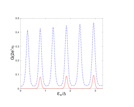
Figure 3: Conductance as a function of $\epsilon_{W}$ at fixed $\Delta_{n}$, $T$ and $\delta_{n}$ for both cases $\xi_{K}\gg L$ (plain style) and $\xi_{K}\ll L$ (dashed style). We have chosen $T\approx\Delta_{n}/10\gg\delta_{n}\approx\Delta_{n}/100$. The curves have been represented on phase but in general they are expected to be shifted, the shift being difficult to determine.

In Figure 3 we sketch the conductance versus $\epsilon_{W}$ in these two cases. In Figure 2, we have drawn schematically the conductance on resonance as a function of temperature for two different bare Kondo temperatures $T_{K,1}^{0}\gg\Delta_{n}$ and $T_{K,2}^{0}\ll\delta_{n}\ll\Delta_{n}$, using the perturbative formula given by Eq. (6) and the Fermi liquid picture valid for the first case only. For the first case, the conductance has a plateau which corresponds to the quantum dot being screened and the $\epsilon$ integral in Eq. (6) averaging over many peaks. The conductance reaches $2e^{2}/h$ only when $T\ll\delta_{n}$. Conversely, in the second case, the conductance remains small till $T\approx\delta$ where the Kondo coupling becomes strongly renormalized (see Eq. (12)). We may expect a very abrupt increase of the conductance in this regime as schematically depicted in Fig 2. Notice that for this choice of $T_{K,2}^{0}$, the renormalized Kondo temperature $T_{K,2}^{R}$ is actually enhanced and of order $\delta_{n}$. These different behaviors lead to different shapes of the curves.

So far, we have considered a device which is symmetric around the quantum dot. This situation might be difficult to reproduce experimentally. One can easily extend this analysis to the non-symmetric case by considering two local densities of states $\rho^{L}$ and $\rho^{R}$. In this case, by tuning $\epsilon_{W}$ it will be difficult to tune simultaneously $\rho_{L}$ and $\rho_{R}$ on resonance. For example, we can reach the situation when $\rho_{L}$ is on resonance and $\rho_{R}$ is not. In the regime $T_{K}^{0}\ll\Delta_{n}$, this implies that the renormalized Kondo temperature is controlled by $\rho_{L}$, meaning that the cloud mainly extends into the left wire. To have both local density of states on resonance, it would in general be necessary to introduce two independent gate voltages $\epsilon_{W}^{L}$ and $\epsilon_{W}^{R}$ controlling the left and right wire.

In conclusion, we have studied how the finite temperature conductance and effective Kondo temperature of a quantum dot embedded in a wire depend strongly on the ratio between the size of the wire and the size of the Kondo screening cloud.

Acknowledgments We would to acknowledge very helpful discussions with A. Balseiro, C. Chamon and L. Glazman.

References

(1) D. Goldhaber-Gordon, H. Shtrikman, D. Mahalu,
D. Abusch-Magder, U. Meirav and M.A. Kaster, Nature 391, 156 (1998).
(2) S.M. Cronewett, T.H. Oosterkamp, L.P. Kouwenhoven,
Science 281, 540 (1998); F. Simmel, R.H. Blick, U.P. Kotthaus,
W. Wegsheider, M. Blichler, Phys. Rev. Lett. 83, 804 (1999).
(3)
W.G. van der Wiel, S. De Franceschi, T. Fujisawa,
J.M. Elzerman, S. Tarucha and L.P. Kouwenhoven, Science, 289, 2105
(2000).
(4) I. Affleck and P. Simon, Phys. Rev. Lett. 86, 2854
(2001).
(5) P. Simon and I. Affleck, Phys. Rev. B64, 085308 (2001).
(6) W. B. Thimm, J. Kroha and J. von Delft, Phys. Rev. Lett. 82 2143 (1999).
(7) P. Nozières,
Proceedings of the 14th International Conference
on Low Temperature Physics, (ed. M. Krusius and M. Vuorio, North-Holland,
Amsterdam, 1975), Vol. 5, p. 339.
(8) A. Kaminski, Yu. V. Nazarov and L. I. Glazman,
Phys. Rev. B 62, 8154 (2000).
(9) P. S. Cornaglia and C. A. Balseiro, cond-mat/0202489.