A novel spin wave expansion, finite temperature corrections and order from disorder effects in the double exchange model.

Abstract

The magnetic excitations of the double exchange (DE) model are usually discussed in terms of an equivalent ferromagnetic Heisenberg model. We argue that this equivalence is valid only at a quasi–classical level — both quantum and thermal corrections to the magnetic properties of DE model differ from any effective Heisenberg model because its spin excitations interact only indirectly, through the exchange of charge fluctuations. To demonstrate this, we perform a novel large $S$ expansion for the coupled spin and charge degrees of freedom of the DE model, aimed at projecting out all electrons not locally aligned with core spins. We generalized the Holstein–Primakoff transformation to the case when the length of the spin is by itself an operator, and explicitly constructed new fermionic and bosonic operators to fourth order in $1/\sqrt{S}$. This procedure removes all spin variables from the Hund coupling term, and yields an effective Hamiltonian with an overall scale of electron hopping, for which we evaluate corrections to the magnetic and electronic properties in $1/S$ expansion to order ${\mathcal{O}}(1/S^{2})$. We also consider the effect of a direct superexchange antiferromagnetic interaction between core spins. We find that the competition between ferromagnetic double exchange and an antiferromagnetic superexchange provides a new example of an ”order from disorder” phenomenon — when the two interactions are of comparable strength, an intermediate spin configuration (either a canted or a spiral state) is selected by quantum and/or thermal fluctuations.

I Introduction

Many magnetic systems of great experimental interest, for example the colossal magnetoresistance (CMR) Manganites [1, 2] and Pyroclhores [3], comprise a band of itinerant electrons interacting with an ordered array of localized magnetic moments with spin $S$. In many cases these systems can be modeled as a single tight band of electrons interacting with localized core spins by a Hund rule exchange interaction, and can be described by a Hamiltonian of the form :

$${\mathcal{H}} = {\mathcal{H}}_{0}+{\mathcal{H}}_{1}+{\mathcal{H}}_{2}$$ (1)

where ${\mathcal{H}}_{0}$ is the bare Hamiltonian for itinerant electrons

$${\mathcal{H}}_{0} = -t\sum_{\langle ij\rangle\alpha}c^{\dagger}_{i\alpha}c_{j\alpha},$$ (2)

${\mathcal{H}}_{1}$ describes the first Hund rule (Kondo type) coupling between localized spins and itinerant electrons

$${\mathcal{H}}_{1}=-J_{H}\sum_{i}\vec{S}_{i}.\vec{s}_{i} \vec{s}_{i}=\sum_{\alpha\beta}c^{\dagger}_{i\alpha}\vec{\sigma_{\alpha\beta}}c_{i\beta}$$ (3)

and ${\mathcal{H}}_{2}$ describes a superexchange between localized spins

$${\mathcal{H}}_{2} = -J_{2}\sum_{\langle ij\rangle}\vec{S}_{i}\vec{S}_{j}$$ (4)

Here the indices $i$ and $j$ run over lattice sites, $\alpha$ and $\beta$ over electron spin states, and components of $\vec{\sigma}_{\alpha\beta}$ are Pauli matrices.

Our primary interest will be to study the limit in which the Hund’s rule coupling $J_{H}$ is positive and is much larger than both $J_{2}$ and $t$. In this case itinerant conduction electrons must be locally aligned with the core spin on any site. As the kinetic energy of electrons is minimal when all electrons are parallel, the core spins are also all parallel, i. e. the ground state is a ferromagnet. The ferromagnetic interaction between core spins mediated by conduction electrons is often referred to as “double exchange”, and the model described by ${\mathcal{H}}_{0}+{\mathcal{H}}_{1}$, in the limit $t/J_{H}\to 0$, is often referred to as the double exchange ferromagnet (DEFM).

Many authors have demonstrated that for classical spins, the fermion-mediated ferromagnetism is described by the effective nearest-neighbor Heisenberg model

$$-J_{1}\sum_{\langle ij\rangle}\vec{T}_{i}.\vec{T}_{j}$$ (5)

with $T=S+x/2$, where $x$ is the electron density, and ferromagnetic exchange integral

$$J_{1}=\frac{\overline{t}}{2S^{2}}$$ (6)

where $\overline{t}$ is the kinetic energy per bond in the lattice, which is a function of the electron doping $x$. In the limit of low electron density $x\to 0$, $\overline{t}\sim tx$.

The aims of this paper are two–fold. Firstly, we discuss the extent to which the DEFM is equivalent to the nearest–neighbor Heisenberg ferromagnet. We argue that this equivalence holds only at infinite $S$, when spin waves are non–interacting quasiparticles. We demonstrate that the interaction between spin waves in the DEFM is qualitatively different from that in the Heisenberg ferromagnet, for which spin waves are exact eigenstates of the Hamiltonian. This difference gives rise to different forms of quantum and thermal corrections to the spin wave dispersion. In particular, we show that spin excitations in the DEFM have a finite lifetime even at $T=0$, i. e. that they cannot be true eigenstates of the Hamiltonian. Physically, the difference between the two models stems from the fact that in a DEFM, the dynamics of the bosonic spin wave modes are completely determined by those of the itinerant electrons. Just as the existence of a finite density of charge carriers generates a dispersion for spin waves about the groundstate of the DEFM, so fluctuations of charge density generate a retarded interaction between these spin waves. Since this interaction is proportional to the charge susceptibility of the itinerant electrons, both its value and the dependence on momentum and frequency are very different from that in the Heisenberg model.

Our second goal is to analyze what happens when the ferromagnetic DE interaction competes with the antiferromagnetic superexchange. The trade–off between fermion-mediated and direct exchanges can, in principle, lead to many different ground states, and indeed numerical studies suggest a very rich phase diagram [4]. Here we address the issue how the system evolves from a DEFM to and AFM with increasing $J_{2}$, provided that there is no phase separation. As observed by de Gennes [5], for classical spins, the configurations which interpolate between FM and AF order are the ones in which the neighbouring lattice spins are misaligned by an angle $\theta$ such that $\cos\theta/2=J_{1}/J_{2}$. This criterium can be satisfied by canting the spins into a two-sublattice state shown in Fig. 1a or into a spiral state shown in Fig. 1b. However, these two configuration are not the only possible as at the classical level we may take any spin of, say, $B$ sublattice of the canted phase and rotate it about the direction of magnetization of the $A$ sublattice without altering the angle between it and the neighbouring spins. This rotation introduces an infinite set of classically degenerate intermediate configurations which interpolate between canted and spiral states. We performed a spin wave analysis of the canted phase using the transformation to bosons described below, and indeed found that a local degeneracy yields a branch of spin wave excitations with $\omega_{sf}(q)=0$ for all $q$. Since it costs no energy to make an excitation, the system cannot distinguish between different states, and is magnetically disordered even at $T=0$[5, 6].

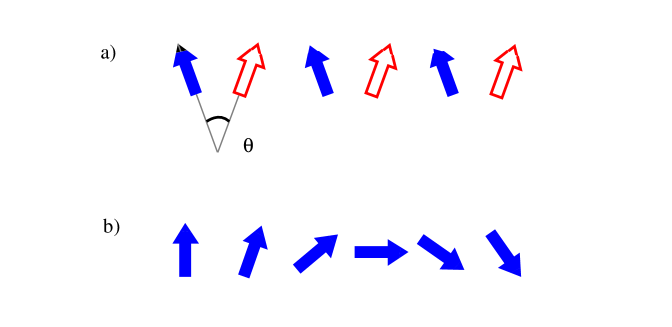
FIG. 1.: Two sublattice canted (a) and spiral (b) spin configurations.

This argument, however, does not hold for quantum spins, and we expect that quantum fluctuations enable the system to choose its true groundstate. A widely studied example of this “order from disorder” behavior is provided by the highly frustrated 2D antiferromagnet on a Kagomé lattice [7]. The question remains as to what kind of order is preferred in our case.

To address this issue we analyzed what is the momentum of the instability of a FM configuration. For classical spins, as discussed above, DE ferromagnetism can be described by the effective exchange model Eq. (5). In this situation, the excitation spectrum in a FM phase is simply

$$\omega_{sw}(q) = zS(J_{1}-J_{2})(1-\gamma_{q})$$ (7)

where $z$ is the lattice coordination number, and

$$\gamma_{q} = \frac{1}{z}\sum_{\delta}e^{i\vec{q}.\vec{\delta}}$$ (8)

where the sum on $\{\vec{\delta}\}$ runs over nearest neighbors vectors. This excitation spectrum vanishes identically for $J_{1}=J_{2}$, in agreement with the infinite degeneracy at $J_{1}<J_{2}$. Suppose now that this degeneracy is lifted by quantum fluctuations, and the spin wave spectrum first becomes unstable at some momentum $Q$. One can easily demonstrate (see below) that if $Q=0$, the resulting state is a spiral, if $Q=(\pi,\pi,\pi)$, the instability leads to a canted state, and if $Q$ is in between the two limits, the system chooses some intermediate spin configuration.

We show that for both small and large electronic densities ($x\ll 1$ or $1-x\ll 1$), the DEFM becomes unstable (with increasing $J_{2}$) against the two–sublattice canted structure. At intermediate densities ($0.05<x<0.68$ in 3D), the first instability is against a spiral spin configuration. Similar results hold for the $2D$ case. We also show that thermal corrections to $\omega_{sw}(q)$ are very different from those in the Heisenberg ferromagnet, and in 3D can be even of a different sign at the lowest densities of carriers. For realistic densities, we found that the functional form of the thermal correction is approximately the same as in the Heisenberg model, but the overall amplitude is substantially increased.

To proceed with the spin wave calculations, we need a “bosonization” scheme which treats both core spins and itinerant electrons on equal footing. Our approach is to transcribe the model Hamiltonian of Eq. (1) in terms of the “natural” collective coordinates of the Kondo coupling term under the assumption that the size of the core spin $S\gg 1$. This procedure has the advantage of making a clean distinction between different types of excitations (spin and charge modes) and of showing clearly the separation of different physical energy scales in the atomic limit. The transformation and its derivation are presented in the next Sec. II. In Sec. III, we apply this transformation to the DE model and discuss the form of the thermal and quantum corrections to the spin wave spectrum. In this section, we also present the results for the damping rate of spin excitations. In Sec. IV, we discuss how quantum and/or thermal fluctuations select an intermediate configuration which interpolates between ferromagnetic state at $J_{1}>J_{2}$ and antiferromagnetic state at vanishing $J_{1}/J_{2}$. We also discuss here a peculiar re-entrant transition between spiral and canted states, which is due to a competition between the selection by thermal and quantum fluctuations. Finally, in Sec. V we present our conclusions.

II Derivation of transformation

Since we wish to work in the limit where the Hund’s rule coupling $J_{H}\gg t$ is the largest energy scale in the problem, it makes sense to treat the onsite Kondo–coupling exactly, and to introduce hopping between sites a perturbation. In the limit where $J_{H}\to\infty$, we can go one step further and project out all electrons not locally aligned with the core spins. We should also define spin wave excitations such that they are the true Goldstone modes of the order parameter, i. e. transverse fluctuations of the composite spin

$$\vec{T}_{i}={\vec{S}}_{i}+\frac{1}{2}\sum_{\alpha\beta}c^{\dagger}_{i\alpha}{\vec{\sigma}}_{\alpha\beta}c_{i\beta}$$ (9)

We can accomplish these goals by first introducing new Fermi operators $f^{\dagger}_{i}$ and $p^{\dagger}_{i}$ which create local states with high ($T=S+1/2$) and low ($T=S-1/2$) total spin $T$, and then generalizing the Holstein–Primakoff transformation to the case where the length of the spin $T$ is itself an operator, introducing a corresponding bosonic operator $\tilde{a}_{i}$. Here we outline this procedure, which was introduced in [8]. A comparison with an exact solution on two sites are given in [9].

Let us start by considering the “Kondo Atom” of a single localized spin and itinerant (spin degenerate) electron orbital

$${\mathcal{H}}_{1}=-J\vec{S}~{}\vec{s}$$ (10)

We can diagonalize this Hamiltonian in by introducing the total spin operator

$$\vec{T} = \vec{S}+\vec{s}$$ (11)

such that

$${\mathcal{H}}_{1} = -\frac{J}{2}\left[\vec{T}^{2}-\vec{S}^{2}-\vec{s}^{2}\right]$$ (12)

$$= -\frac{J}{2}\left[T(T+1)-S(S+1)-s(s+1)\right]$$ (13)

Here the quantum number for the “itinerant” electron $\vec{s}$ can take on values $s=\{0,1/2\}$, and the total spin quantum number $T=\{S+1/2,S,S-1/2\}$, so we find three corresponding energy eigenvalues

$$\lambda = \left\{-\frac{JS}{2},0,\frac{JS}{2}\left(1+\frac{1}{S}\right)\right\}$$ (14)

where the state with total spin $S$ and eigenvalue zero is doubly degenerate and corresponds to zero or double occupancy of the itinerant electron state.

We can now define a new quantization axis for a composite spin $T$ and introduce the corresponding “up” ($f$) and “down” ($p$) fermionic states. The magnitude of $T$ is then

$$T=S+\frac{f^{\dagger}f-p^{\dagger}p}{2}$$ (15)

This procedure corresponds to making an $SU(2)$ rotation of the electron spin coordinates such that the new quantization axis follows the direction of the instantaneous local magnetization. Accordingly, one approach to deriving an effective action for the DE model is to work in the $SU(2)$ rotated local frame and introduce a gauge field to describe the rotation of coordinates for an electron hopping along any given bond of the lattice (see e. g. [14]).

For our purposes, it is however more advantageous to use a somewhat different procedure. First we note that to leading order in $1/S$, the states with $T=S\pm 1/2$ correspond to aligning or antialigning the spin of a single itinerant electron with the localized spin on that site. At this level, we can replace the Kondo coupling with a local magnetic field and reduce ${\mathcal{H}}_{1}$ to ${\mathcal{H}}_{1}=\tilde{{\mathcal{H}}}_{1}+const$ where

$$\tilde{{\mathcal{H}}}_{1} \approx -\frac{JS}{2}\left[f^{\dagger}f-p^{\dagger}p\right]$$ (16)

Second, we observe that we can obtain the correct eigenvalues of the full quantum mechanical problem by keeping (15) and modifying the simple “Zeeman–splitting” form of Eq. (16) to

$$\tilde{{\mathcal{H}}}_{1} = -\frac{JS}{2}\left[f^{\dagger}f-p^{\dagger}p\left(1+\frac{1}{S}\right)+\frac{f^{\dagger}fp^{\dagger}p}{S}\right]$$ (17)

One can easily make sure that Eq. (17) yields correct eigenstates (14) for any $S$. The new local interaction

$$-\frac{J}{2}f^{\dagger}fp^{\dagger}p$$ (18)

comes from the fact that the eigenvalues of ${\mathcal{H}}_{1}$ for $T=S\pm 1/2$ are not symmetric about zero. Physically, it implies that if the system has both $f$ and $p$ electrons it can save energy for positive $J$ by putting them on the same site to male a total spin of length $T=S$.

We see that if $J$ is the largest parameter in the problem and $S$ is large (as we assume), the fermionic states created by the $p-$operator are separated in energy by $J(S+1/2)$ from fermionic states created by $f-$operator,and can be safely eliminated from the low–energy sector. This is the obvious advantage of introducing $f-$ and $p-$ operators. The problem which we now have to solve is how to relate these two operators, which describe fermionic states of a composite spin $T$ to the “original” up/down fermionic operators $c_{\uparrow}=u$, $c_{\downarrow}=d$ introduced with respect to a quantization axis of the core spin $S$. We solve this last problem order by order in $1/S$ by introducing two sets of Holstein–Primakoff bosons — one $a$ for a core spin $\vec{S}$ and another $\tilde{a}$ for the composite spin $\vec{T}$. Introducing the quantization axis $z$ for the core spin and the corresponding fermionic states $c_{\uparrow}=u$, $c_{\downarrow}=d$, we have

$$S^{z} = S-a^{\dagger}a$$ (19)

$$S^{+} = \sqrt{2S}\sqrt{1-\frac{a^{\dagger}a}{2S}}a$$ (20)

$$S^{-} = \sqrt{2S}a^{\dagger}\sqrt{1-\frac{a^{\dagger}a}{2S}}$$ (21)

and

$$T^{z}= S^{z}+\frac{u^{\dagger}u-d^{\dagger}d}{2} =T-\tilde{a}^{\dagger}\tilde{a}$$ (22)

$$T^{+}= S^{+}+u^{\dagger}d =\sqrt{2T}\sqrt{1-\frac{\tilde{a}^{\dagger}\tilde{a}}{2T}}\tilde{a}$$ (23)

$$T^{-}= S^{-}+d^{\dagger}u =\sqrt{2T}\tilde{a}^{\dagger}\sqrt{1-\frac{\tilde{a}^{\dagger}\tilde{a}}{2T}}$$ (24)

where $[a,a^{\dagger}]=[\tilde{a},\tilde{a}^{\dagger}]=1$. The relation between $a$, $u$,$d$ and $\tilde{a}$, $f$ and $p$ then follows from Eq. (15) on the magnitude of the composite spin, commutation relation for fermionic and bosonic operators and the constraints that the total number of particles be conserved

$$f^{\dagger}f+p^{\dagger}p = u^{\dagger}u+d^{\dagger}d$$ (25)

and that double or zero occupancy of the electron orbital correspond to the same two sets of states state in either representation

$$f^{\dagger}p^{\dagger}=u^{\dagger}d^{\dagger}\qquad etc.$$ (26)

This set of constraints is sufficient to uniquely define the transformation, and after lengthly algebra we find :

$$\tilde{a} = a\left[1+\frac{d^{\dagger}d-u^{\dagger}u}{4S}+\frac{3u^{\dagger}u-5d^{\dagger}d+2u^{\dagger}ud^{\dagger}d}{32S^{2}}\right]+\frac{u^{\dagger}d}{\sqrt{2S}}\left(1-\frac{1}{4S}\right)-\frac{d^{\dagger}u}{\sqrt{2S}}\frac{aa}{4S}$$ (27)

$$f = u\left[1-\frac{a^{\dagger}a+d^{\dagger}d}{4S}+\frac{3d^{\dagger}d+3a^{\dagger}a-2d^{\dagger}da^{\dagger}a-a^{\dagger}a^{\dagger}aa}{32S^{2}}\right]+\frac{da^{\dagger}}{\sqrt{2S}}\left(1-\frac{1}{4S}\right)$$ (28)

$$p = d\left[1-\frac{a^{\dagger}a+uu^{\dagger}}{4S}+\frac{3uu^{\dagger}+3a^{\dagger}a-2uu^{\dagger}a^{\dagger}a-a^{\dagger}a^{\dagger}aa}{32S^{2}}\right]-\frac{ua}{\sqrt{2S}}\left(1-\frac{1}{4S}\right)$$ (29)

To verify the transformation, we checked that it correctly reproduces the Kondo coupling term on a single site. In terms of original $a$, $u$, and $d$ operators, the Hamiltonian for a Kondo “atom” reads :

$${\mathcal{H}}_{1}=-\frac{JS}{2} \left((1-\frac{a^{\dagger}a}{S})[u^{\dagger}u-d^{\dagger}d]+\sqrt{\frac{2}{S}}\sqrt{1-\frac{a^{\dagger}a}{2S}}ad^{\dagger}u+\sqrt{\frac{2}{S}}a^{\dagger}\sqrt{1-\frac{a^{\dagger}a}{2S}}u^{\dagger}d\right)$$ (30)

Substituting the transformation, we indeed found that in terms of new $\tilde{a}$, $f$ and $p$ it exactly reproduces Eq. (17).

For purposes of developing a calculation scheme based on these coordinates we need the corresponding inverse transformation. This is found to be identical up to the sign of terms at odd order in $1/\sqrt{S}$ :

$$a = \tilde{a}\left[1+\frac{p^{\dagger}p-f^{\dagger}f}{4S}+\frac{3f^{\dagger}f-5p^{\dagger}p+2f^{\dagger}fp^{\dagger}p}{32S^{2}}\right]-\frac{f^{\dagger}p}{\sqrt{2S}}\left(1-\frac{1}{4S}\right)+\frac{p^{\dagger}f}{\sqrt{2S}}\frac{\tilde{a}\tilde{a}}{4S}$$ (31)

$$u = f\left[1-\frac{\tilde{a}^{\dagger}\tilde{a}+p^{\dagger}p}{4S}+\frac{3p^{\dagger}p+3\tilde{a}^{\dagger}\tilde{a}-2p^{\dagger}p\tilde{a}^{\dagger}\tilde{a}-\tilde{a}^{\dagger}\tilde{a}^{\dagger}\tilde{a}\tilde{a}}{32S^{2}}\right]-\frac{p\tilde{a}^{\dagger}}{\sqrt{2S}}\left(1-\frac{1}{4S}\right)$$ (32)

$$d = p\left[1-\frac{\tilde{a}^{\dagger}\tilde{a}+ff^{\dagger}}{4S}+\frac{3ff^{\dagger}+3\tilde{a}^{\dagger}\tilde{a}-2ff^{\dagger}\tilde{a}^{\dagger}\tilde{a}-\tilde{a}^{\dagger}\tilde{a}^{\dagger}\tilde{a}\tilde{a}}{32S^{2}}\right]+\frac{f\tilde{a}}{\sqrt{2S}}\left(1-\frac{1}{4S}\right)$$ (33)

The inverse transformation Eqs. (31–33) can be applied whenever the Hamiltonian Eq. (1) has a magnetically ordered ground state, and since all Fermi and Bose operators are well defined, is an ideal starting point for constructing a diagrammatic perturbation theory of spin and charge excitations in such a system, and for calculating response functions of the DE model in a controlled way.

For the simplest possible case of two core spins sharing a single electron, the model Eq. (1) can be solved exactly [2], and one of us has checked explicitly that our expansion scheme reproduces all features of the exact solution, order by order in $1/\sqrt{S}$ [9].

III spin wave excitations in the Double Exchange model

We now return to the DE model and analyze the form of the spin wave dispersion using the transformation derived above. As discussed, for a ferromagnetic Kondo coupling $J_{H}$ and $t/J_{H}\rightarrow 0$, $p-$operators can be safely neglected. The effective Hamiltonian for the DEFM is therefore found by substituting the inverse transformation Eqs. (31–33) into Eq. (1) and dropping all $p$ operators. Corrections at finite $t/J_{H}$ will be discussed elsewhere. Substituting the transformation into the DE Hamiltonian ${\mathcal{H}}={\mathcal{H}}_{0}+{\mathcal{H}}_{1}$ and expanding in $1/S$ we obtain in terms of the new $f$ and $\tilde{a}$ operators

$${\mathcal{H}} = {\mathcal{H}}_{0}^{\prime}+{\mathcal{H}}_{2}+{\mathcal{H}}_{4}+{\mathcal{O}}(1/S^{3})$$ (34)

$${\mathcal{H}}_{0}^{\prime} = -zt\sum_{\langle ij\rangle}f^{\dagger}_{i}f_{j}$$ (35)

$${\mathcal{H}}_{2} = \frac{zt}{4S}\sum_{\langle ij\rangle}f^{\dagger}_{i}f_{j}\left[\left(\tilde{a}^{\dagger}_{i}\tilde{a}_{i}+\tilde{a}^{\dagger}_{j}\tilde{a}_{j}\right)\left(1-\frac{3}{8S}\right)-2\tilde{a}^{\dagger}_{i}\tilde{a}_{j}\left(1-\frac{1}{2S}\right)\right]$$ (36)

$${\mathcal{H}}_{4} = \frac{zt}{32S^{2}}\sum_{\langle ij\rangle}f^{\dagger}_{i}f_{j}\left[\tilde{a}^{\dagger}_{i}\tilde{a}^{\dagger}_{i}\tilde{a}_{i}\tilde{a}_{i}+\tilde{a}^{\dagger}_{j}\tilde{a}^{\dagger}_{j}\tilde{a}_{j}\tilde{a}_{j}-2\tilde{a}^{\dagger}_{i}\tilde{a}_{i}\tilde{a}^{\dagger}_{j}\tilde{a}_{j}\right]$$ (37)

On Fourier transform we obtain :

$${\mathcal{H}}_{0}^{\prime} = \sum_{k_{1}}(\epsilon_{1}-\mu)f^{\dagger}_{1}f_{1}$$ (38)

$${\mathcal{H}}_{2} = \frac{1}{N}\sum_{k_{1}\ldots k_{4}}v^{13}_{24}f^{\dagger}_{1}f_{2}\tilde{a}^{\dagger}_{3}\tilde{a}_{4}\delta_{1+3-2-4}$$ (40)

$$v^{13}_{24}=\frac{1}{4(S+\frac{1}{2})}\left[\left(1+\frac{1}{8S}\right)\left(\epsilon_{1+3}+\epsilon_{2+4}\right)-\left(\epsilon_{1}+\epsilon_{2}\right)\right]$$

$${\mathcal{H}}_{4} = \frac{1}{32S^{2}}\frac{1}{N^{2}}\sum_{\vec{k}_{1}\ldots\vec{k}_{6}}f^{\dagger}_{1}f_{2}\tilde{a}^{\dagger}_{3}\tilde{a}^{\dagger}_{4}\tilde{a}_{5}\tilde{a}_{6}.v^{134}_{256}.\delta_{1+3+4-2-5-6}$$ (43)

$$v^{134}_{256}=\frac{1}{4}\left[\epsilon_{1+3-5}+\epsilon_{1+3-6}+\epsilon_{1+4-5}+\epsilon_{1+4-6}-4\epsilon_{1}\right.$$

$$\qquad\qquad\left.\quad\epsilon_{2+6-4}+\epsilon_{2+6-3}+\epsilon_{2+5-4}+\epsilon_{2+5-3}-4\epsilon_{2}\right]$$

All energy scales are set by the electron dispersion, which for the simple tight binding kinetic energy term Eq. (2), is given by $\epsilon_{k}=-zt\gamma_{k}$.

We see that the original problem of spinfull electrons interacting with quantum mechanical localized spins reduces to a single band of spinless fermions interacting with a reservoir of (initially dispersionless) bosonic spin modes. For this last problem we can evaluate all quantities of physical interest diagrammatically, starting from the bare bosonic Green’s function given by

$${\mathcal{D}}_{0}(q,i\Omega_{n})=(i\Omega_{n})^{-1}$$ (44)

and the bare $f$ electron Green’s function

$${\mathcal{G}}_{0}(k,i\omega_{n})=(i\omega_{n}-\epsilon_{k}+\mu)^{-1}$$ (45)

We note that since operators $\tilde{a}^{\dagger}$ and $\tilde{a}$ describe fluctuations of the composite spin, the pole in the fully renormalized bosonic propagator ${\mathcal{D}}(q,i\Omega_{n})$ coincides with the pole in the transverse spin susceptibility, i. e. ${\mathcal{D}}(q,i\Omega_{n})$ describes true spin wave excitations. Higher-order terms in the Holstein-Primakoff expansion of the composite spin $T$ in terms of $\tilde{a}^{\dagger}$ and $\tilde{a}$ only give rise to the incoherent background in the spin susceptibility but do not affect the pole. This separation between the pole and the incoherent background only makes sense if the damping of spin waves is negligible small. We will show that the spin wave damping appears only at $O(1/S^{3})$ such that to order $O(1/S^{2})$ (to which we will perform controlled calculations), nonlinear terms in the Holstein-Primakoff transformation for $T$ can be neglected [10].

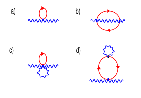
FIG. 2.: a)–d) Diagrams contributing to spin wave self energy in Ferromagnet to order ${\mathcal{O}}(1/S^{2})$. Only diagrams a) and b) are physically relevant. Diagram c) cancels unphysical leftovers from the diagrams a) and b), and diagram d) accounts for thermal renormalization of the chemical potential and the exchange integral $J_{1}$ but does not change the form of the spin wave dispersion.

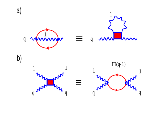
FIG. 3.: The representation of the diagram Fig 2b as an effective four–boson interaction mediated by the charge suscpetibility (particle–hole polarization bubble).

The dispersionless form of ${\mathcal{D}}(q,i\Omega_{n})$ does not survive self-energy corrections arising from interaction with Fermions — the bosonic self-energy depends on momentum $q$, and this dependence gives rise to a dispersion of the spin wave excitations. Physically, this dispersion is generated by the fact that any departure from perfect ferromagnetic ordering of composite spins costs kinetic energy. The form of this dispersion should be appropriate to a ferromagnet on a lattice, i. e. it should have a set of Goldstone modes with energy $\omega_{sw}(q)$ scaling as $q^{2}$ in the zone center, and be continuous across the zone boundary.

The perturbation theory for the bosonic propagator $D(q,\Omega)$ is straightforward. We have $D^{-1}(q,\Omega)=\Omega-\Sigma(q,\Omega)$. The lowest-order (in $1/S$) contribution to $\Sigma(q,\Omega)$ comes from a single loop of fermions, and this evaluates to

$$\Sigma^{(1a)}(q) = zJ_{1}S[1-\gamma(\vec{q})]$$ (46)

where

$$J_{1} = \frac{t}{2S^{2}}\frac{1}{N}\sum_{\vec{k}}n_{k}\gamma(\vec{k})$$ (47)

The result for $J_{1}$ can be rewritten as $J_{1}=\overline{t}/(2S^{2})$ where $\overline{t}$ is the magnitude of the Fermionic kinetic energy per bond on the lattice.

The classical spin wave dispersion of the DEFM, Eq. 46 corresponds exactly to what we would expect for a nearest neighbour Heisenberg model with exchange integral $J_{1}$. The equivalence of the DEFM and the nearest neighbour Heisenberg model at ${\mathcal{O}}(1/S)$ was first discussed by de Gennes [5] and results for classical spin wave dispersion have been rederived by many other authors since [11, 13, 14, 15, 16].

We can translate the energy scale for zero temperature spin wave dispersion into a mean field transition temperature for a Heisenberg FM using the relation

$$T_{c} = \frac{zS(S+1)}{3}J_{1}$$ (48)

giving approximate transition temperature for a $d$ dimensional quarter filled cubic lattice with bandwidth These estimates are in surprisingly good correspondence with transition temperatures for the real CMR materials.

We now demonstrate that the DE and Heisenberg models are not equivalent beyond ${\mathcal{O}}(1/S)$. To check this, we need to go a step further and compute the spin wave dispersion to order ${\mathcal{O}}(1/S^{2})$. For this, we must include the ${\mathcal{O}}(1/S^{2})$ contribution of the one–loop diagram Fig. 2a and also two–loop self–energy diagrams. The two–loop diagrams are presented in Fig. 2b–d. The first of these diagrams represents the bosonic self–energy due to the effective four–boson interaction mediated by the Pauli susceptibility of fermions. The diagram in Fig. 2c is the first–order contribution from the six–fold, $1/S^{2}$ term in Eq. (38). This diagram is physically uninteresting, and is only necessary to restore the Goldstone theorem. The diagram Fig. 2d accounts for thermal renormalization of the chemical potential and the exchange integral $J_{1}$ but does not change the functional form of the spin wave dispersion. We neglect this diagram below.

We see that from physics perspective, the relevant diagram is Fig. 2b. This diagram can be thought of as a first order bosonic self–energy due to effective four–boson interaction mediated by fermions (see Fig. 3a–b). The relation between DEFM and the Heisenberg model then can be readily understood on general grounds. Indeed, in a HFM, the four–boson vertex does not depend on frequency and scales as $J_{1}q^{2}l^{2}$ (Ref. [17]) where $q,l\ll 1$ are the bosonic momenta. In the DEFM, the interaction is mediated by the dynamical charge susceptibility of the Fermi gas, $\Pi(q-l,\omega_{p}-\omega_{l})$ (see Fig. 3(b)), which is generally a complex function of momentum and frequency. This gives rise to two effects which both are relevant to our analysis:

(i) $\Pi(q-l,\omega_{p}-\omega_{l})$ has a branch cut, which gives rise to a nonzero renormalization of the spin wave dispersion at $T=0$, and

(ii) the static $\Pi(q-l,0)$, relevant to thermal corrections to the dispersion at $T<J_{1}S$, scales differently from $J_{1}$ and this changes the scale of the self–energy in the DEFM relative to a classically equivalent HFM. In particular, at small $p_{F}$, $J_{1}\propto p^{3}_{F}$, while $\Pi(q-l)\propto p_{F}$ at $q,l_{typ}\ll p_{F}$ and $\Pi(q-l)\propto p^{3}_{F}/|q-l|^{2}$ for $|q-l|\gg p_{F}$. Thermal corrections to spin wave dispersion in the DEFM are therefore enhanced relative to the HFM. Furthermore, at small doping $x$, when typical $q$ and $l$ exceed $p_{F}$, the momentum dependence of $\Pi(q-l)$ causes thermal self energy correction in the DEFM to have a different functional form from that in the HFM.

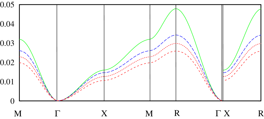
FIG. 4.: Dispersion of spin waves in a cubic DEFM with electron doping $x=0.7$ and spin $S=3/2$, in units of the electron bandwidth $2zt=1.0$. Solid line — dispersion of classically equivalent Heisenberg model. Dashed lines — dispersion of DEFM including leading quantum and thermal corrections for (top to bottom) $T=0$, $T=2D/3$ and $T=D$ where $D=12J_{1}S$ is the bandwidth of spin wave excitations.

We now proceed with the calculations. Assembling all three ${\mathcal{O}}(1/S^{2})$ contributions to the self-energy and splitting it into quantum and thermal pieces, we obtain after some algebra that all unwanted terms are canceled out and the Goldstone mode at $q=0$ survives, as required. The resulting self–energy is given by

$$\Sigma^{(2)}(q,\omega)\approx\Sigma^{(2)}(q) = \Sigma^{(2)}_{T=0}(q)+\Sigma^{(2)}_{T}(q)$$ (49)

where

$$\Sigma^{(2)}_{T=0}(q) = -\frac{zt}{4S^{2}}\frac{1}{N^{2}}\sum_{pl}n_{F}(p)[1-n_{F}(l)]\left[(1-\gamma_{q})\gamma_{p}\frac{\gamma_{p}+\gamma_{l}}{\gamma_{p}-\gamma_{l}}-\frac{\gamma^{2}_{p}-\gamma^{2}_{k+p}}{\gamma_{p}-\gamma_{l}}\right]$$ (50)

and

$$\Sigma^{(2)}_{T}(q) = -\frac{zt}{4S^{2}}\frac{1}{N^{2}}n_{F}(p)n_{B}(l)\left[\frac{(\gamma_{p}-\gamma_{p+q})(\gamma_{p+q-l}-\gamma_{p+q})}{\gamma_{p}-\gamma_{p+q-l}}+\frac{(\gamma_{p}-\gamma_{p+l})(\gamma{p+l-q}-\gamma_{p+l})}{\gamma_{p}-\gamma_{p+l-q}}\right]$$ (51)

Here $n_{F}(k)=n_{F}(\epsilon_{k})$ and $n_{B}(q)=n_{B}(\Omega(q))$ are Fermi and Bose distribution functions, respectively. The frequency dependence of the self–energy is relevant for the computations of the bosonic damping which is of order $1/S^{3}$ (see below), but can be neglected in the computations to order $1/S^{2}$ as typical bosonic $\omega$ are of order $\omega_{sf}(q)\propto t/S$ and are small by $1/S$ compared to typical fermionic energies which are of order $t$. In this situation, the full bosonic dispersion is simply

$$\omega_{sw}(q)=zJ_{1}S(1-\gamma_{q})+\Sigma^{2}(q).$$ (52)

We will also neglect the temperature dependence of the Fermi functions as we are interested in temperatures of order the spin wave bandwidth $T\sim t/S\ll t$. This makes possible the simple separation of the self energy into thermal and quantum pieces as written in Eq. (49). We now analyze quantum and thermal corrections to spin wave dispersion. We begin with the case of zero temperature.

A Quantum corrections at $T=0$

1 spin wave dispersion

We see from (50) that at $T=0$, the interaction with the charge degrees of freedom leads to an overall reduction in the spin wave bandwidth (the first term in (50)), together with a modification in the form of the dispersion provided by the second term in in (50). This second term

$$\Delta\Sigma^{(2)}(q) = \frac{zt}{4S^{2}}\frac{1}{N^{2}}\sum_{pl}n_{F}(p)[1-n_{F}(l)]\frac{\gamma^{2}_{p}-\gamma^{2}_{k+p}}{\gamma_{p}-\gamma_{l}}$$ (53)

is either positive or negative throughout the Brillouin zone, depending on doping, and has the symmetry $\Delta\Sigma^{(2)}(q)=\Delta\Sigma^{(2)}(\pi-q)$ which bare spin wave dispersion does not possess. Near the center of the Brillouin zone it behaves as

$$\Delta\Sigma^{(2)}(q\approx 0)\sim\frac{t}{2S^{2}}I(x)q^{2}$$ (54)

where

$$I(x)=\frac{1}{N^{2}}\sum_{k_{1}k_{2}}\frac{\gamma_{1}^{2}}{\gamma_{1}-\gamma_{2}}\left[1-n_{F}(k_{2})\right]n_{F}(k_{1})$$ (55)

is a doping dependent constant. By symmetry, the behaviour of $\Delta\Sigma^{(2)}(q)$ near the zone corner $q\approx\pi$ must have exactly the same form. Along the zone diagonal

$$\Delta\Sigma^{(2)}(q) = \frac{zt}{4S^{2}}I(x)\left[1-\cos(2q)\right]$$ (56)

This form is very similar to the form of correction to Heisenberg dispersion found in numerical studies of the DE model on a ring [18].

For a small density of electrons ($x<0.31$), $I(x)>0$ in both 2D and 3D, and corrections to dispersion lead to a “softening” of modes at the zone boundary relative to those the zone center. The same is true for small density of holes $1-x<0.07$ in $2D$ and $1-x<0.06$ in $3D$. For intermediate densities $0.31(7)<x<0.92(7)$ in $2D$, and $0.31(7)<x<0.94(2)$ in $3D$, $I(x)$ is negative, i. e. quantum effects cause a relative softening of spin wave modes at $q=0$. These results are in good agreement with earlier numerical studies studies [20]. We discuss the consequences of the non–monotonic doping dependence of $I(x)$ in more detail later in Sec. IV when we consider order from disorder effects.

We note in passing that if we formally extend our $1/S$ results to arbitrary $S$, the spin wave dispersion becomes unstable for $S<S_{cr}$ where in 3D $S_{cr}=(1/2N)\sum_{k}(1+\gamma_{k})/(1-\gamma_{k})\approx 1$. This opens up a possibility that for small S (e.g., $S=1/2$), the ground state may not be a ferromagnet, as suggested by some numerical studies [19]. However, the extension to small $S$ is beyond the scope of the present paper.

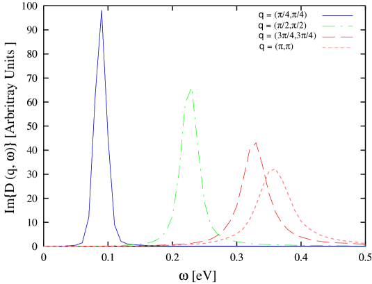
FIG. 5.: Numerical results for the imaginary part of $D(q,\omega)$ of a $2D$ double exchange ferromagnet with $S=3/2$ and doping of $0.18$ holes per site, with energy in units of the hopping integral $t$. The plots show the increasing damping of spin waves along the zone diagonal. Sharp structure in the data is an artifact of finite numerical resolution and has been partially removed by convolution with a Gaussian of width $0.01t$.

2 Damping of spin waves

While spin waves are exact eigenstates of the Heisenberg Hamiltonian (5), in the DEFM only the $q=0$ (Goldstone) mode is an eigenstate. All other spin wave modes in the DEFM have a finite lifetime, even at zero temperature. Physically, the possibility for a spin wave to decay at $T=0$ is again related to the presence of Fermions. A spin wave with energy $\omega_{sw}(q)$ can give energy to a particle–hole pair, and decay into a lower energy spin wave — the process described by the diagram Fig. 2b. As a consequence $\Sigma^{(2)}(q,\Omega)$ contains an imaginary part which describes the damping of a spin wave.

To calculate damping effects it is necessary to keep the bosonic energies $\Omega$, $\omega_{q}^{{}^{\prime}}$ together with the fermionic $\epsilon_{k}$ in the denominator of $\Sigma^{(2)}(q,\Omega)$. This means that the calculations are formally less controlled, as we include terms one order smaller in $1/S$. To work rigorously at this order it would be necessary to extend the (inverse) transformation Eq.(31–33) to ${\mathcal{O}}(1/S^{3})$ — a very involved task. However the physical origin of the damping is clear, and we verified that the imaginary part of the self–energy to ${\mathcal{0}}(1/S^{3})$ is fully captured by just keeping $\Omega$ in denominators of two–loop self–energy diagrams. We then obtain

$$\Sigma^{\prime\prime}_{T=0}(q,\Omega) = \Theta(\Omega)\frac{\pi}{(4S)^{2}}\frac{1}{N^{2}}\sum_{kq^{\prime}}\left(\epsilon_{k+q^{\prime}}+\epsilon_{k}-2\epsilon_{k+q}\right)^{2}n_{F}(k+q^{\prime})[1-n_{F}(k)]\delta\left((\Omega-\omega_{q-q^{\prime}})-(\epsilon_{k+q^{\prime}}-\epsilon_{k})\right)$$ (57)

where we have grouped together terms of ${\mathcal{O}}(0)$ and terms of ${\mathcal{O}}(1/S)$ within the argument of the delta function.

Without $\Sigma^{\prime\prime}(q,\Omega)$, the imaginary part of the bosonic propagator $D(q,\Omega)$ is just a delta function dispersing with the spin wave energy $\omega_{sw}(q)$, i. e.

$$D^{\prime\prime}(q,\Omega) = -\pi\delta(\Omega-\omega_{sw}(q))$$ (58)

However because of the non–zero $\Sigma^{\prime\prime}(q,\Omega)$, the simple delta function peak (58) is replaced by a broader dispersing feature with is approximately Lorentzian in shape with the maximum at $\omega_{sw}(q)$.

We can obtain an estimate of the width of $D^{\prime\prime}(q,\Omega)$ by calculating the damping of spin waves on the mass shell

$$\Gamma_{q} = \frac{\pi}{4S^{2}}\frac{1}{N^{2}}\sum_{kq^{\prime}}\left(\epsilon_{k}-\epsilon_{k+q}\right)^{2}n_{F}(k+q^{\prime})[1-n_{F}(k)]\delta\left((\omega_{sw}(q)-\omega_{sw}(q-q^{\prime}))-(\epsilon_{k+q^{\prime}}-\epsilon_{k})\right).$$ (59)

where we have used the delta function on energy to eliminate terms of subleading order in $1/S$ from the vertex. The damping of spin waves must vanish for $q\to 0$, in order for the Goldstone theorum to be satisfied. For $q\ll p_{F}$ we find that $\Gamma_{q}$ vanishes as $\omega_{sw}(q)~{}q^{d+1}\sim q^{d+3}$. A factor $\omega_{sw}(q)$ comes from the 2D integration over $d|k-k_{F}|$ and $d|q^{\prime}|$, another factor $q^{2}$ comes from the vertex, and the remaining factor $q^{d-1}$ comes from the fact that $|q^{\prime}|\leq q$ and hence $d^{d}q^{\prime}\sim q^{d-1}d|q^{\prime}|$. In 2D, this yields $\Gamma_{q}\propto q^{5}$ and in 3D, $\Gamma_{q}\propto q^{6}$. This fully agrees with earlier estimates [21, 16]. This strong dependence on $q$ survives up to $q\sim p_{F}$. At larger $q$, and $p_{F}\ll 1$, the damping of spin waves saturates at a constant value $\Gamma_{q}\propto(t/S^{3})$. At $p_{F}\sim 1$, $\Gamma_{q}$ at $q\geq p_{F}$ is in general a rather complicated function of momentum.

In Fig. 5 we plot the imaginary part of $D(q,\Omega)$ obtained by numerically evaluating (57) for a set of momenta on the zone diagonal for a DEFM on a 2D square lattice, for $S=3/2$ and electron density $x=0.82$. From the plot, we see that zone corner modes are clearly broadened relative to those in the zone center. Evaluating $\Gamma_{q}$ throughout the BZ for a range of dopings in 2D we obtain a functional form of damping similar to that recently reported in [16]. However our estimate on the upper bound for values of damping is about $25\%$ smaller than that given in [16].

The results for the 3D cubic case are similar, and best summarized by plotting the $\Gamma_{q}$ along all major symmetry directions. In Fig. 6 we plot the damping for a cubic system with electron doping $x=0.7$ and spin $S=3/2$, in units of the electron bandwidth $2zt=1.0$. The damping of spin waves is small at low $q$, but strongly momentum dependent. Damping is large for $q$ approaching the zone edge, and has a maximum value of about $10\%$ of the spin wave dispersion at the zone corner. Stationary points of the damping (maxima, minima and points of inflection) occur at symmetry points of the the BZ or where $q$ crosses the Fermi surface.

The large absolute value of the damping at large $q$ in the DEFM and its strong momentum dependence is consistent with the experimental behavior seen in Neutron scattering experiments on the Manganites, where damping is large, highly momentum dependent, and can rise to $\sim 10\%$ of spin wave dispersion at the zone corner [25].

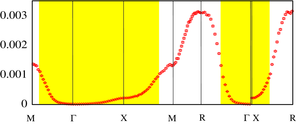
FIG. 6.: Damping of the spin wave on the mass shell as a function of momentum throughout the BZ for a cubic DEFM with electron doping $x=0.7$ and spin $S=3/2$, in units of the electron bandwidth $2zt=1.0$. The volume enclosed by the Fermi surface is denoted by shading.

B Thermal corrections at $T>0$

We now discuss the form of the correction to the spin wave dispersion at finite $T$. Continuing the spirit of comparison with the low $T$ expansion for a Heisenberg FM, we assume that $T\leq J_{1}S\ll t$. In a nearest–neighbor Heisenberg FM the thermal renormalization of the spin wave dispersion to first order in $1/S$ is

$$\Sigma^{(2)}_{T}(q) = -\frac{1}{4S}~{}\omega_{sw}(q)B\left(\frac{T}{J_{1}S}\right)$$ (60)

where [17]

$$B\left(\frac{T}{J_{1}S}\right)=\frac{1}{N}\sum_{l}n_{B}(l)(1-\gamma_{l})$$ (61)

At the lowest temperatures,

$$B\left(\frac{T}{J_{1}S}\right)\approx\frac{\zeta(5/2)}{32\pi^{3/2}}~{}\left(\frac{T}{J_{1}S}\right)^{5/2}$$ (62)

We see that the dispersion preserves its $T=0$ form, and that thermal fluctuations only reduce the overall scale of dispersion by an amount which at low $T$ is proportional to $T^{5/2}$. For the DEFM we find below that at small $x$, the form of $\Sigma^{(2)}_{T}(q)$ is totally different from that in HFM. For finite $x$, we find that $\Sigma^{(2)}_{T}(q)$ can be crudely approximated by the same functional formulas (62), but the overall factor has completely different doping dependence from the effective exchange coupling $J_{1}$.

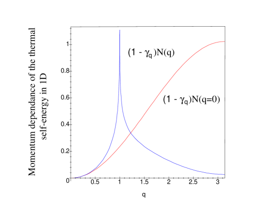
FIG. 7.: The momentum dependence of the thermal correction to spin-wave dispersion in a DEFM in 1D for $p_{F}=0.4$, following Eq. (67).

We now proceed with the analysis of Eq. (51). In general, at finite $T$ there are three typical momenta in the problem, the spin wave momentum $q$, the Fermi momentum $p_{F}$, and a thermal length scale $l_{typ}\sim(T/J_{1}S)^{1/2}$ (in units where the lattice constant $a=1$). Let us consider first the case when $T$ is very low and $l_{typ}\sim(T/J_{1}S)^{1/2}$ are smaller than $p_{F}$. This case mimics the behavior at intermediate electron densities. Expanding in (51) in $l$ we obtain after a simple algebra:

$$\Sigma^{(2)}_{T}(q)=\frac{t}{4S^{2}}\sum_{l}n_{B}(l)l^{2}\sum_{p}n_{F}(p)\gamma_{p}\Psi(p,q)$$ (63)

where

$$\Psi(p,q)=1+\gamma_{q}-\frac{4}{z^{2}}\sum_{i}\frac{\sin^{2}(p_{i}+q_{i})+\sin^{2}(p_{i})}{\gamma_{p}(\gamma_{p}-\gamma_{p+q})}+\frac{\sin^{2}(p_{i}-q_{i})+\sin^{2}(p_{i})}{\gamma_{p}(\gamma_{p}-\gamma_{p-q})}$$ (64)

where $i$ takes the values $x,y$ and $z$. If $\Psi(p,q)$ was just proportional to $1-\gamma_{q}$, the thermal self-energy would have the same functional form as in HFM. We see, however, that $\Psi(p,q)$ is more complex and depends on both variables.

The form of $\Psi(p,q)$ is particularly simple in 1D. Here we obtain from Eq. (64)

$$\Psi(p,q) = (1+\cos q)-\frac{\sin^{2}(p+q)+\sin^{2}(p)}{\cos p(\cos p-\cos(p+q))}-\frac{\sin^{2}(p-q)+\sin^{2}(p)}{\cos p(\cos p-\cos(p-q))}$$ (66)

$$=-(1-\cos q)\frac{1+2\sin^{2}p+\cos q}{1-\cos q-2\sin^{2}p}$$

We see that at small $q$ and finite $p$, $\Psi(p,q)$ scales as $q^{2}$ as it indeed should. Substituting the result for $\Psi(p,q)$ into (63) we find after integrating over $p$

$$\Sigma^{(2)}_{T}(q)=-\frac{t}{4S^{2}}\left(\sum_{l}n_{B}(l)l^{2}\right)~{}(1-\cos q)~{}N(q)$$ (67)

where

$$N(q)=\frac{\sin p_{F}}{\pi}\left(-1+\frac{1}{2\sin p_{F}\sin q/2}\log\frac{\sin p_{F}+\sin q/2}{|\sin p_{F}-\sin q/2|}\right)$$ (68)

At $q\rightarrow 0$,

$$N(q)\rightarrow\frac{1}{\pi}~{}\left(\frac{1}{\sin p_{F}}-\sin p_{F}\right).$$ (69)

At the zone boundary, $q=\pi$,

$$N(\pi)=\frac{\sin p_{F}}{\pi}\left(-1+\frac{1}{2\sin p_{F}}\log{\frac{1+\sin p_{F}}{1-\sin p_{F}}}\right).$$ (70)

At small $p_{F}$, $N(\pi)=(1/3\pi)\sin^{3}p_{F}+...$. We see that $N(q)>0$, and hence $\Sigma^{(2)}_{T}(q)$ is negative, i. e. thermal fluctuations reduce the spin wave energy. This agrees with the spin wave result for the HFM.

In Fig. 7 we plot the form of thermal corrections to spin wave dispersion for a DEFM in 1D with $p_{F}=0.4$, together with a correction proportional to $1-\gamma_{q}$ having the same prefactor at small $q$. We clearly see two effects — the suppression of temperature corrections at large $q$ relative to small $q$, and a logarithmic singularity coming from the perfect nesting of the Fermi surface in 1D.

The $q^{2}$ behavior at the smallest $q$ exists in all dimensions as we have explicitly verified. The explicit forms are, however, rather complex and we refrain from presenting them. It is essential that for all $D$, the prefactor scales as $1/p^{2}$ for $q\ll p\ll 1$. In 3D, the $q^{2}/p^{2}$ form of $\Psi(p,q)$ yields for $q,l\ll p_{F}\leq 1$,

$$\Sigma^{(2)}_{T}(q)=-\frac{tq^{2}p_{F}}{144\pi^{2}S^{2}}\frac{1}{N}\sum_{l}n_{B}(l)l^{2}\propto q^{2}p_{F}T^{5/2}$$ (71)

In 2D, we obtained

$$\Sigma^{(2)}_{T}(q)=-\frac{tq^{2}}{48\pi S^{2}}\frac{1}{N}\sum_{l}n_{B}(l)l^{2}\propto q^{2}T^{2}$$ (72)

Since the overall scale of spin wave dispersion in the DEFM at low doping is proportional to $x$, (which scales as $p_{F}^{2}$ in 2D and $p_{F}^{3}$ in 3D), we see that the overall scale of thermal corrections in the DEFM is enhanced by a factor $1/p_{F}^{2}$ relative to a Heisenberg model with the effective FM coupling $J_{1}$.

Numerical results for the spin wave dispersion in a cubic system with an electron doping of $x=0.7$, including thermal corrections, are shown in Fig. 4. Thermal corrections are generally small compared with the quantum corrections at $T=0$, the two effects becoming comparable only for $T\sim 6J_{1}S$.

It is helpful to divide thermal self energy corrections in the DEFM by the thermal corrections for a Heisenberg model with the same spin stiffness $J_{1}S$, i. e. to consider

$$\alpha(q,x,T) = \frac{4S}{B(T/J_{1}S)}~{}\frac{\Sigma^{(2)}_{T}(q)}{\omega_{sw}(q)}$$ (73)

We plotted this ratio against reduced temperature $T/J_{1}S$ for several $q$ and and a range of dopings $0.1<x<0.9$ in Fig. 8. We see that for a wide range of dopings and reduced temperatures the data for different $q$ collapse onto a single “universal” surface. This means that $\alpha$ remains roughly constant as a function of $T/J_{1}S$, and also depends only weakly on on $q$, which implies that for the experimentally relevant intermediate dopings, the thermal self-energy in a DEFM roughly mimics that in a HFM. Still, however, the overall amplitudes of the corrections are very different for the reasons given above. We found that the ratio of the two is approximately constant at $\alpha\approx 5$ for $0.25<x<0.75$, falling away to about $\alpha=2$–$3$ for $x=0.1$ ($x=0.9$). These numbers should be compared to enhancement of corrections by a factor $2$–$3$ relative to a nearest neighbour HFM observed in La_0.85Pb_0.15MnO₃ [22], for which $x=0.85$. The authors of [22] interpreted the enhancement of temperature corrections in La_0.85Pb_0.15MnO₃ in terms of effective non–nearest neighbour couplings — we note that these are dynamically generated by the form of interaction between spin waves in the DEFM — see Fig. 3(b). At the smallest dopings $\alpha$ acquires a strong dependence on both $q$ and $T/J_{1}S$, as discussed below. We also found that for $D=2$ and $D=1$, the deviations from $\alpha\approx const$ are more prominent for the same intermediate $x$. In particular, in 1D a simple experimentation with trigonometry yields $N(\pi)<N(0)$. This implies that compared to the HFM, the strength of thermal fluctuations in DEFM is reduced near $q=\pi$.

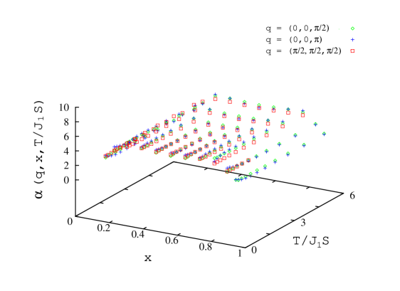
FIG. 8.: Ratio of thermal corrections to spin wave dispersion in a DEFM to the thermal corrections of a classically equivalent Heisenberg FM $\alpha(q,x,T)=\Sigma^{DEFM}_{T}(q)/\Sigma^{HFM}_{T}(q)$ for momenta $q=(0,0,\pi/2)$, $q=(0,0,\pi)$ and $q=(\pi/2,\pi/2,\pi/2)$ as a function of doping $x$ and reduced temperature $T/J_{1}S$. Plot shows that data for a wide range of dopings, momenta and reduced temperatures approximately collapse onto a “universal” surface.

We now consider analytically what happens if we lift the restrictions that both $q$ and $l_{typ}\sim T/J_{1}S$ are smaller than $p_{F}$. As we still focus on low $T\leq J_{1}S$, $p_{F}$ should also be small which in turn implies that electron density $x\ll 1$. We verified that the results similar to the ones below also hold for small hole density $1-x\ll 1$.

Let us first consider what happens when $q$ exceeds $p_{F}$. In this limit, we can approximate $\Psi(p,q)$ by $\Psi(0,q)$. Substituting the result into the expression for the self-energy, we obtain, in any D

$$\Sigma^{(2)}_{T}(q)=-\frac{t~{}x}{4S^{2}}\frac{1}{N}\sum_{l}n_{B}(l)l^{2}P(q)$$ (74)

where

$$P(q)=\left[\frac{2}{z}\frac{1-\gamma_{2q}}{1-\gamma_{q}}-(1+\gamma_{q})\right]$$ (75)

In 1D, (74) reduces to

$$\Sigma^{(2)}_{T}(q)=-\frac{t~{}x}{4S^{2}}\frac{1}{N}\sum_{l}n_{B}(l)l^{2}(1+\cos q)$$ (76)

This result coincides with Eq. (67) as for $p_{F}\ll 1$ and $q\gg p_{F}$, $N(q)$ from (68) reduces to $N(q)=x(1+\cos q)/(1-cosq)$ where $x=p_{F}/\pi$.

In 3D, Eqn (74) yields $\Sigma^{(2)}_{T}(q)\propto p^{3}_{F}T^{5/2}$. In 2D, we have $\Sigma^{(2)}_{T}(q)\propto p^{2}_{F}T^{2}$. Comparing these results with Eq. (71) and (72), we see that the at $q\gg p_{F}$, the self-energy is reduced by $p^{2}_{F}/q^{2}$, relative to corrections at the zone center. This is precisely the result we anticipated on general grounds as when $q$ exceeds $p_{F}$, the effective boson–boson vertex is reduced due to the reduction of the charge susceptibility which mediates boson–boson interaction. Note that this reduction eliminates the quadratic dependence on $q$, i. e. the thermal self-energy becomes flat at $q\gg p_{F}$.

Curiously enough, in 3D, at these low dopings, $P(q)$ is negative for all $q$ along zone diagonal ($P(q)=-(1/3)(1-\cos q)$), i. e. the thermal self-energy changes sign compared to Eq. (71). In 2D, $P(q)$ vanishes along zone diagonal, and in 1D, $P(q)=1+\cos q$ is positive shown above (see Eq. (76).

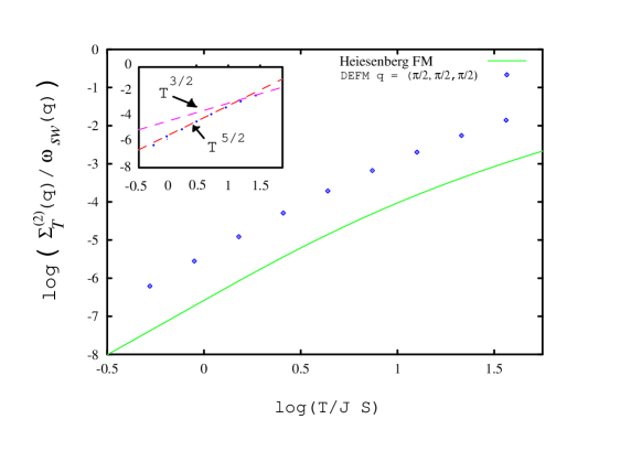
FIG. 9.: Thermal corrections to spin wave dispersion in a cubic DEFM with $x=0.67$ for $q=(\pi/2,\pi/2,\pi/2)$ (points) compared with those for a classically equivalent Heisenberg FM (solid line). While the functional form of the corrections is similar, their magnitudes are very different. The inset shows the crossover from $T^{5/2}$ behavior at low $T$ to $T^{3/2}$ behavior at $T\geq J_{1}S$.

The reduction of the bosonic self–energy due to the reduction of the charge susceptibility at large momenta can also be detected by analyzing the form of $\Sigma^{(2)}_{T}$ when $q$ is smaller than $p_{F}$, but $l_{typ}$ exceeds $p_{F}$. This case is even more instructive than the large $q$ and small $l_{typ}$ limit, as $\Sigma^{(2)}_{T}$ can be obtained analytically for arbitrary ratio of $l_{typ}$ and $p_{F}$. Indeed, expanding in all three momenta in (51) we obtained in 3D

$$\Sigma^{(2)}_{T}(q)=-\frac{tq^{2}p_{F}}{144\pi^{2}S^{2}}\frac{1}{N}\sum_{l}n_{B}(l)l^{2}\Phi_{3D}\left(\frac{l}{2p_{F}}\right)$$ (77)

The scaling function $\Phi_{3D}(y)$ is given by

$$\Phi_{3D}(y)=\frac{3}{y^{2}}\left[\int_{z_{min}}^{1}dz\sqrt{1-y^{2}(1-z^{2})}(1+2y^{2}z^{2})-1\right]$$ (78)

For $y<1$, $z_{min}=0$, for $y>1$, $z_{min}=\sqrt{(y^{2}-1)/y^{2}}$. Evaluating the integral analytically in the limiting cases, we find $\Phi_{3D}(y\rightarrow 0)=1,~{}\Phi_{3D}(y=1)=0$, $\Phi_{3D}(y\gg 1)\approx-1/y^{2}$. The $y=0$ limit reproduces Eq. (71). For large $y$, i. e. for $q\ll p_{F}\ll(T/J_{1}S)^{1/2}$, we have $\Sigma^{(2)}_{T}(q)=Cq^{2}p^{3}_{F}(T/J_{1}S)^{3/2}$ where $C>0$. The scaling function $\Phi_{3D}(y)$ is shown in Fig. (11). The sign change of $\Phi_{3D}(y)$ between small and large $y$ collaborates our earlier observation that in 3D, the self-energy at the smallest $T$ and at $T/J_{1}S\geq p_{F}$ have different signs. When $q$ exceeds $p_{F}$ and become comparable to $(T/J_{1}S)^{1/2}$, Eq. (77) becomes invalid, and $\Sigma^{(2)}_{T}(q)$ smoothly interpolates into $\Sigma^{(2)}_{T}(q)\propto p^{3}_{F}T^{5/2}$, as in Eq. (74).

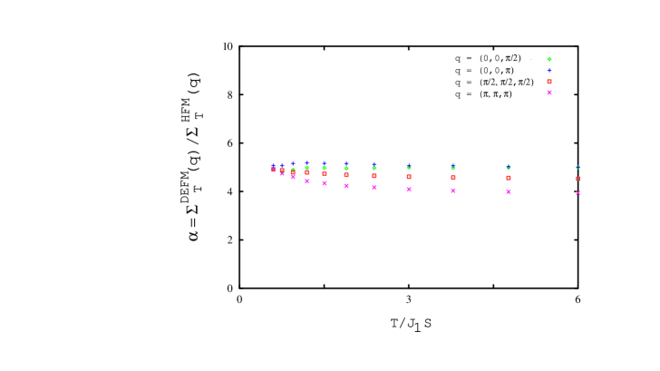
FIG. 10.: Thermal corrections to spin wave dispersion in a DEFM with $x=0.67$ normalized to those in an equivalent HFM for $q=(0,0,\pi/2)$, $q=(0,0,\pi)$,$q=(\pi/2,\pi/2,\pi/2)$ and $q=(\pi,\pi,\pi)$.

A very similar behavior holds in 2D case. Here we obtained

$$\Sigma^{(2)}_{T}(q)=-\frac{tq^{2}}{48\pi S^{2}}\frac{1}{N}\sum_{l}n_{B}(l)l^{2}\Phi_{2D}\left(\frac{l}{2p_{F}}\right)$$ (79)

where

$$\Phi_{2D}(y) = 1,~{}~{}y<1$$ (80)

$$\Phi_{2D}(y) = -\frac{3}{2y^{2}}+\frac{1}{\pi y^{3}}\int_{0}^{\phi_{max}}\frac{d\phi}{\cos\phi}\sqrt{1-(y\sin{\phi})^{2}}(1+2y^{2}+4(y\cos\phi)^{2}),~{}~{}y>1$$ (81)

where $\sin{\phi_{max}}=1/y$. In the limit $y\gg 1$, we found analytically $\Phi_{2D}(y)=a/y^{4}$ with $a>0$.

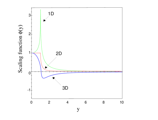
FIG. 11.: Scaling function governing thermal corrections to spin wave dispersion in the DEFM in 1D — Eq. (83), 2D — Eq. (80) and 3D — Eq. (78).

Again, when $q$ exceeds $p_{F}$ and becomes comparable to : $(T/J^{*}S)^{1/2}$, Eq. (79) becomes invalid, and $\Sigma^{(2)}_{T}(q)$ smoothly interpolates into $\Sigma^{(2)}_{T}(q)\propto p^{3}_{F}T^{5/2}$ as in Eq.(74).

Finally, in 1D,

$$\Sigma^{(2)}_{T}(q)=-\frac{tq^{2}}{8\pi S^{2}p_{F}}\frac{1}{N}\sum_{l}n_{B}(l)l^{2}\Phi_{1D}\left(\frac{l}{2p_{F}}\right)$$ (82)

where

$$\Phi_{1D}(y)=\frac{1}{2y}\log{\frac{1+y}{|1-y|}}.$$ (83)

In the two limits, $\Phi_{1D}(0)=1$, and $\Phi_{1D}(y\gg 1)=1/y^{2}$. As before, when $q$ exceeds $p_{F}$ and becomes comparable to $(T/J^{*}S)^{1/2}$, Eq. (82) smoothly interpolates into Eq. (76).

We see that in any D, the Heisenberg form of the correction to the spin wave dispersion is reproduced only at small $(T/J_{1}S)^{1/2}\ll p_{F}$, when the scaling function $\Phi(y)$ can be approximated by a constant. At larger temperatures $y_{typ}\sim(T/J_{1}Sp^{2}_{F})^{1/2}$ become large, and the variation of $\Phi(y)$ cannot be neglected. The only difference between different $D$ is that $\Phi_{3D}(y)$ changes sign at $y=O(1)$ and becomes negative at large $y$, while $\Phi_{2D}$ and $\Phi_{1D}$ remain positive for all $y$.

Unfortunately, the new physics we just described is confined to very small $x$in D=3. This is simply because in 3D $p_{F}=(6\pi^{2}x)^{1/3}$, and to make $p_{F}$ small, one needs a very small x. For such small $x$, our numerical analysis is not very accurate, but we were able to confirm that $\Sigma^{(2)}_{T}(q)$ changes sign as $T$ increases. We also clearly detected the downturn renormalization of $|\Sigma^{(2)}_{T}(q)|$ with increasing $T$ at $x$ (or $1-x$) $\sim 0.1$.

IV Order from disorder in the double exchange model

We now apply the results of the previous section to study the order from disorder phenomenon in the double exchange model. We recall that if double exchange ferromagnetism $J_{1}$ is put into competition with direct antiferromagnetic superexchange $J_{2}$ between core spins, then classically, ferromagnetic state becomes unstable at $J_{1}<J_{2}$, but the intermediate configuration is not specified — the only requirement on classical spins is that neighboring spins are misaligned by an angle $\Theta$:

$$\cos\Theta=J_{1}/J_{2}.$$ (84)

This condition allows an infinite set of intermediate states. The two limits of this set are canted and spiral spin configurations, as discussed in the introduction.

We first demonstrate that at a classical level, the spin wave excitation spectrum of either canted or spiral state indeed contains a zero-energy branch of excitations. Consider for definiteness a canted phase. The bosonic Hamiltonian for a two sublattice canted structure described by the full ${\mathcal{H}}_{0}+{\mathcal{H}}_{1}+{\mathcal{H}}_{2}$ at vanishing $t/J_{H}$ and $J_{2}/J_{H}$ can be obtained directly within our expansion scheme. Working to ${\mathcal{O}}(1/S)$ and introducing two quantization axes misaligned by $\theta/2$, we obtain

$${\mathcal{H}}_{\theta} = {\mathcal{H}}^{(0)}_{\theta}+{\mathcal{H}}^{(1)}_{\theta}+{\mathcal{H}}^{(2)}_{\theta}+\ldots$$ (85)

where

$${\mathcal{H}}^{(0)}_{\theta} = \sum_{\langle ij\rangle}\left\{-t\cos\frac{\theta}{2}\left[f^{\dagger}_{Ai}f_{Bj}+\mbox{\it h.\ c.\ }\right]+J_{2}S^{2}\cos\theta\right\}$$ (86)

$${\mathcal{H}}^{(1)}_{\theta} = \sum_{\langle ij\rangle}\left\{\frac{t}{\sqrt{2S}}\sin\frac{\theta}{2}\left[f^{\dagger}_{Ai}f_{Bj}\left(\tilde{b}_{j}-\tilde{a}^{\dagger}_{i}\right)+\mbox{\it h.\ c.\ }\right]\right.$$ (88)

$$-J_{2}S\sqrt{\frac{S}{2}}\left.\sin\theta\left[\left(\tilde{b}_{j}-\tilde{a}^{\dagger}_{i}\right)+\mbox{\it h.\ c.\ }\right]\right\}$$

$${\mathcal{H}}^{(2)}_{\theta} = \sum_{\langle ij\rangle}\left\{\frac{t}{4S}\cos\frac{\theta}{2}\left[f^{\dagger}_{Ai}f_{Bj}\left(\tilde{a}^{\dagger}_{i}\tilde{a}_{i}+\tilde{b}^{\dagger}_{j}\tilde{b}_{j}-2\tilde{a}^{\dagger}_{i}\tilde{b}_{j}\right)+\mbox{\it h.\ c.\ }\right]\right.$$ (90)

$$+J_{2}S\left.\left[\cos\theta\left(\tilde{a}^{\dagger}_{i}\tilde{a}+\tilde{b}^{\dagger}_{j}\tilde{b}_{j}\right)-\cos^{2}\frac{\theta}{2}\left(\tilde{a}^{\dagger}_{i}\tilde{b}_{j}+\tilde{b}^{\dagger}_{j}\tilde{a}_{i}\right)+\sin^{2}\frac{\theta}{2}\left(\tilde{a}_{i}\tilde{b}_{j}+\tilde{b}^{\dagger}_{j}\tilde{a}^{\dagger}_{i}\right)\right]\right\}$$

where $f_{A}$ denotes a local “up spin” electron on sublattice $A$, $\tilde{b}$ a Holstein-Primakoff boson on sublattice $B$, etc., and the sum over $\langle ij\rangle$ is restricted to pairs of neighbouring sites with site $i$ on the $A$ sublattice and site $j$ on the $B$ sublattice. We note that the effective Hamiltonian for the antiferromagnetic Néel state is obtained by setting $\theta=\pi$ above.

To zeroth order in $1/S$ the ground state energy of this configuration is

$$E_{0} = 2Nz\left[J_{2}S^{2}\cos\theta-\overline{t}\cos\frac{\theta}{2}\right]$$ (91)

Minimizing this with respect to $\theta$ gives the de Gennes result (Eq. 84) for the canting angle.

The spin wave dispersion to leading order in $1/S$ is obtained in the same way as for a ferromagnet, by evaluating the leading corrections to an (initially dispersionless) bosonic propagator. This spin wave “spectrum” is doubly degenerate, and the lattice momentum $\vec{q}$ is restricted to the reduced Brillouin appropriate to the two sublattice spin configuration. The evaluation of the self-energy to order $1/S$ is technically a bit more involved than for a ferromagnet as in addition to the one-loop self-energy from ${\mathcal{H}}^{(2)}_{\theta}$ we also need to compute the second-order contribution from ${\mathcal{H}}^{(1)}_{\theta}$. The last term vanishes at zero momentum after one substitutes the canting angle, as it indeed should, but it does contribute at second order. We found that the two contributions exactly cancel each other, i. e. to order $1/S$,

$$\omega_{sw}(\vec{q}) \equiv 0$$ (92)

The vanishing of the leading order spin wave dispersion is clearly linked to the degeneracy of the classical groundstate, and, as we already mentioned in the introduction, has a simple physical interpretation — at the classical level we may take any spin on the $B$ sublattice and rotate it about the direction of magnetization of the $A$ sublattice without altering the angle between it and the neighbouring spins. As $\theta$ does not change, this perturbation does not cost any energy, and by extension the spin wave dispersion at ${\mathcal{O}}(1/S)$ is zero [5, 6].

We now proceed to the computations beyond the leading order in $1/S$. Our key goal is to understand which configuration of the classically degenerate set is selected by either quantum or thermal fluctuations. There are two ways to attack this problem. First, we may continue with the analysis of the canted phase and perform computations to next order in $1/S$. This is possible but requires a lot of efforts as at each order there is a competition between the contributions from from the term quartic and bosons and the term linear in bosons. A second route which we choose is to analyze the momentum of the instability of the ferromagnetic configuration. To ${\mathcal{O}}(1/S)$, the excitation spectrum of a ferromagnet in the presence of the antiferromagnetic exchange is given by Eq. (7) which vanishes identically for $J_{1}=J_{2}$, in agreement with the infinite degeneracy of the classical groundstate for $J_{1}<J_{2}$. We already know, however, that the excitation spectrum of the DE model is different from that of a ferromagnet and, depending on the density of electrons, is softened either at the zone boundary or at $q=0$.

A way to understand what this implies is to analyze what form of the spin wave dispersion one generally expects at a point where a ferromagnet becomes unstable towards either canted or spiral phases, if there were no degeneracy. The simplest way to eliminate a degeneracy is to formally add an exchange interaction between second neighbors

$$H_{3} = J_{3}\sum_{\langle ij\rangle^{\prime}}\vec{S}_{i}\vec{S}_{j}$$ (93)

This extra interaction modifies the dispersion Eq. (7) to give

$$\omega_{sw}(q) = zS(J_{1}-J_{2})(1-\gamma_{q})-zSJ_{3}(1-\gamma_{2q})$$ (94)

For positive $J_{3}$ (antiferromagnetic next–nearest neighbour exchange), the $J_{3}$ term favors maximum misalignment of the next–nearest neighbour spins. This condition is best satisfied by the spiral state. For negative $J_{3}$, the extra coupling favors parallel orientation of next–nearest neighbour spins. This is a property of the canted phase. Analyzing the dispersion in the presence of $J_{3}$ we immediately see that for positive $J_{3}$, the spectrum first becomes unstable at $q=0$, at $J_{1}=J_{2}+4J_{3}$, while for negative $J_{3}$, the excitation spectrum first softens at $J_{1}=J_{2}$ at $q=(\pi,\pi,\pi)$. Performing the classical spin wave analysis for the full DE Hamiltonian with extra $J_{2}$ and $J_{3}$ terms slightly below the instability we find that for positive $J_{3}$, the spin wave spectrum has three zero modes: at $q=0$ and an incommensurate momenta ${\vec{q}}=\pm(q_{0},q_{0},q_{0})$ where $q_{0}=\theta$. This is exactly what we expect in a spiral state. For negative $J_{3}$, the soft modes remain at $q=0$ and at $(\pi,\pi,\pi)$. This is what we expect in a two-sublattice canted phase.

The above analysis shows that the type of the ground state configuration below the instability can be obtained by just analyzing the spin wave spectrum at the instability point of the ferromagnetic phase. Using the results from the previous section we find that at $T=0$, the instability occurs when

$$\tilde{\omega}_{sw}(q) = zS(J_{1}-J_{2})[1-\gamma(q)]+\Delta\Sigma^{(2)}(q,0)=0$$ (95)

where, as shown, $J_{1}=\overline{t}/2S^{2}$ with $\overline{t}=tN^{-1}\sum_{k}n_{k}\gamma_{k}$, and the relevant self–energy correction is presented in Eq. (50). As discussed in Section III, this can be split into two of two pieces. One scales as $1-\gamma(q)$ and just renormalize $J_{1}$. The second piece $\Delta\Sigma^{(2)}(\vec{q})$ accounts for the renormalization of the form of the dispersion. It reads

$$\Delta\Sigma^{(2)}(\vec{q}) = 4\frac{zt}{(4S)^{2}}\frac{1}{N^{2}}\sum_{12}\frac{\gamma_{1}^{2}-\gamma_{1+q}^{2}}{\gamma_{1}-\gamma_{2}}n_{1}(1-n_{2})$$ (96)

The first instability of the DEFM will occur for some value of $J_{2}$ sufficient to cancel the bare spin dispersion and this quantum correction. The value of critical $J_{2}$ depends on the form of $\Delta\Sigma^{(2)}$ as a function of $q$ and doping $x$. We therefore consider the ratio

$$\lambda_{q}^{x}=\frac{\Delta\Sigma^{(2)}(q)}{1-\gamma(q)}$$ (97)

as a function of doping. The wavevector $q=q^{*}$ for which $\lambda_{q}^{x}$ has its minimum value defines the momentum of the instability.

Near $q=0$, we obtain using (54) and (55)

$$\lambda_{q\approx 0}^{x}=\frac{t}{2S^{2}}~{}\frac{I(x)q^{2}}{q^{2}/z}=\frac{zt}{2S^{2}}I(x)$$ (98)

while at the zone corner

$$\lambda_{q\approx\pi}^{x}=\frac{t}{2S^{2}}~{}\frac{I(x)q^{2}}{2-(\pi-q)^{2}/z}\to 0$$ (99)

Whether the first instability occurs in the zone center or the zone corner therefore depends on the sign of $I(x)$. As we discussed in Sec III), $I(x)$ is positive for $x<0.31$ in both 2D and 3D, and for small density of holes $1-x<0.07$ in $2D$ and $1-x<0.06$ in $3D$. For these dopings, the intermediate configuration is then a canted phase. For intermediate densities $0.31(7)<x<0.92(7)$ in $2D$, and $0.31(7)<x<0.94(2)$ in $3D$, $I(x)$ is negative, i. e. quantum effects cause a relative softening of spin wave modes at $q=0$, and the intermediate configuration is a spiral phase. These results are in good agreement with earlier numerical studies studies [20].

At finite temperature, the range of dopings where the canted phase is selected increases with $T$ as for realistic $x$, classical fluctuations primarily soften the dispersion near $q=0$ and hence favor the spiral state, at least at small $T$. At higher $T$, and in $D=3$, thermal fluctuations may in principle, cause a re–entrant transition into a spiral phase as when $T$ becomes larger than $J_{H}Sp^{2}_{F}$, the sign of $\Sigma^{(2)}_{T}(q)$ changes, and thermal fluctuations now favor the canted phase. In practice, however, we found that this sign change occurs at unrealistically large $T$ for which our low $T$ analysis is inapplicable.

We conclude this section with few words of caution. First, in our analysis we assumed that there are no nontrivial transitions inside the intermediate phase, i. e. the configuration which becomes the ground state immediately after ferromagnetic instability yields to another configuration at some distance away from the instability. Such a possibility exists in general, but to the best of our knowledge, there is no known example of such behavior. Second, we neglected phase separation [23]. To study this possibility in our approach, one has to analyze the sign of the longitudinal susceptibility in, e.g. the canted phase. If it is negative, then the system is unstable towards phase separation [24]. These calculations are currently under way.

V Conclusions

We have performed a novel large $S$ expansion for the Kondo model on a magnetically ordered lattice, and presented a simple, physically transparent and controlled calculation scheme for evaluating corrections to magnetic and electronic properties of the model to ${\mathcal{O}}(1/S^{2})$. Calculations are particularly straightforward in the limit where the onsite (ferromagnetic) Kondo coupling $J_{H}$ greatly exceeds the electron bandwidth $zt$ (the double exchange model). In this limit we have used our expansion scheme to study quantum and thermal corrections to the spin wave spectrum of the double exchange ferromagnet. We argue that a double exchange ferromagnet is equivalent to a Heisenberg model with effective coupling $J_{1}\propto t/S^{2}$ only at a quasi–classical level — both quantum and thermal corrections to the spin wave spectrum of a double exchange ferromagnet differ from any effective Heisenberg model because its spin excitations interact only indirectly, through the exchange of charge fluctuations. We demonstrated that the effective interaction between spin waves is mediated by Pauli susceptibility of electrons which has a much larger amplitude than $J_{1}$ and also has its own non–analytic momentum and frequency dependence. We argued that at $T=0$, the nonanalyticity in the frequency dependence of the effective vertex gives rise to a finite self-energy correction which changes the momentum dependence of the spin wave dispersion compared to that in a Heisenberg ferromagnet. The form of the full dispersion which we found is similar to that found in numerical studies of the DE model [18]. For a small density of electrons, or small density of holes, the corrections to dispersion lead to a “softening” of modes at the zone boundary relative to those the zone center. For intermediate densities, quantum effects cause a relative softening of spin wave modes at $q=0$. These results are in good agreement with earlier numerical studies  [20].

The softening of zone boundary spin waves has been observed in neutron scattering experiments on the CMR Manganites [25] at $x\sim 0.7$. It has been suggested that this softening may be due to deviations from Heisenberg behavior in the DEFM [18, 25], the influence of optical phonons [26], or due to orbital degrees of freedom [27]. Our analysis argues against the first possibility as for $x\sim 0.7$, our zero temperature theory predicts a relative hardening rather than softening of the dispersion at $(\pi,\pi,\pi)$. We note however that the leading corrections to spin wave dispersion at finite $t/J_{H}$ do lead to a softening of zone boundary modes [28].

We also found that the process by which spin waves decay into lower energy spin excitations dressed with particle–hole pairs leads to a finite spin wave lifetime at $T=0$. The spin wave lifetime is very long at low $q$, scaling as $q^{-4}$ in 3D for $p_{F}>q\to 0$, but increases rapidly with increasing $q$. The large absolute value of the damping at large $q$ in the DEFM and its strong momentum dependence is consistent with the experimental behavior in the Manganites [25].

We then analyzed in detail the form of the temperature corrections to the spin wavespin wave dispersion. We argued that for experimentally relevant densities, the corrections roughly have the same functional form as in a Heisenberg ferromagnet, but the overall scale is much larger. At low density (small $p_{F}$), for which an analytic treatment is possible, thermal corrections in DEFM are enhanced relative to those in a HFM with the same effective exchange coupling $J_{1}$ by a factor proportional to $1/p^{2}_{F}$. At very small $p_{F}$, we also found that not only the amplitude but also the functional form of the thermal self-energy in DEFM is qualitatively different from that in a HFM. In 3D, the thermal self-energy in DEFM at low doping even changes sign relative to that in a HFM. The enhancement of temperature the overall scale corrections relative to a HFM has been observed experimentally in La${}_{0}.85$Sr${}_{0}.15$MnO₃ [22], and we believe that our finite temperature results will be useful for the interpretation of the neutron data on Manganites.

We also considered the effect of a direct superexchange antiferromagnetic interaction between core spins. We find that the competition between ferromagnetic double exchange and an antiferromagnetic superexchange provides a new example of an “order from disorder” phenomenon — when the two interactions are of comparable strength, an intermediate spin configuration (either a canted or a spiral state) is selected only by quantum and/or thermal fluctuations. We discussed which configurations are selected at various dopings.

The issue left for further study is the possibility of a phase separation in the intermediate regime into ferromagnetic and antiferromagnetic regions [4, 29], and also possible stripe formation at low hole doping. The analysis of these issues is clearly called for.

Acknowledgments.

It is our pleasure to acknowledge helpful conversation with S. W. Cheong, D. Golosov, R. Joynt, M. Kagan, T. A. Kaplan, G. Khaliullin, S. D. Mahanti, A. Millis, E. Müller-Hartmann, M. Norman, O. Tchernyshyov, N. B. Perkins, N. M. Plakida and M. Rzchowski. This work was supported under NSF grant DMR–9632527 and the visitors program of MPI–PKS (N. S.), and by NSF grant DMR-9979749 (A. V. C.).

REFERENCES

- [1] C. Zener, Phys. Rev. 82, 403 (1951).
- [2] P. W. Anderson and H. Hasegawa Phys. Rev. 100, 675 (1955).
- [3] P. Majumdar and P. Littlewood, Phys. Rev. Lett. 81, 1314 (1998).
- [4] J. Riera, K. Hallberg and E. Dagotto, Lett. 79, 713 (1997).
- [5] P.–G. de Gennes, Phys. Rev. 118, 141 (1960).
- [6] D. Golosov, Phys. Rev. B 58, 8617 (1998).
- [7] A. B. Harris, C. Kallin and A. J. Berlinsky, Phys. Rev. B 45, 2899 (1992); S. Sachdev, Phys. Rev. B 45, 12377 (1992); A. V. Chubukov, Phys. Rev. Lett. 69, 832 (1992).
- [8] Nic Shannon and Andrey Chubukov, J. Phys. Condens. Matt, 14 L235 (2002).
- [9] Nic Shannon, J. Phys. Condens. Matt, 13 6731 (2001).
- [10] This is indeed true for the computations of the transverse spin correlator between different sites. For a Kondo problem at a given site, higher–order terms in the Holstein–Primakoff expansion for a composite spin are indeed relevant as they preserve the correct spin algebra, and are incorporated into our transformation in Sec. II.
- [11] K. Kubo and N. Ohata, J. Phys. Soc. Jpn. 33, 21 (1972).
-
[12]
E. L. Nagaev
Phys. Rev. B 58, 827 (1998);
“Physics of Magnetic Semiconductors”, Moscow, Mir Publ (1979). - [13] N. Furukawa, J. Phys. Soc. Jpn. 63, 3214 (1994).
- [14] A. J. Millis, P. B. Littlewood and B. I. Schraimann Phys. Rev. Lett. 74, 5144 (1995).
- [15] N. B. Perkins and N.M. Plakida, Theor. Math. Phys., 120 (1999) 1182.
- [16] D. Golosov, Phys. Rev. Lett. 84, 3974 (2000).
- [17] see e.g., Akhiezer et al “Spin waves”, Wiley, NY (1968).
- [18] T. A. Kaplan and S. D. Mahanti, J. Phys. Condens. Matt. 9 L291 (1997).
- [19] J. Zang et al, J. Phys. Condens. Matt. 9, L157 (1997) and references therein.
- [20] P. Wurth and E. Müller-Hartmann, Europhys. J. B 5, 403 (1998); D. Golosov, J. Appl. Phys. 87, 5804 (2000).
- [21] V. Yu Irkhin and M. I. Katsnel’son JETP 88, 522 (1985).
- [22] L. Vasiliu–Doloc et. al. Phys. Rev. B 58, 14913 (1998).
- [23] A. Moreo, S. Yunoki and E. Dagotto, Science 283, 2034 (1999).
- [24] B.I. Shraiman and E. Siggia, Phys. Rev. B 46, 8305 (1992); A. Chubukov and K. Musaelian, Phys. Rev. B 51 12605 (1995).
- [25] H. Y. Hwang et. al. , Phys. Rev. Lett. 80, 1316 (1998), Tapan Chatterji, private communication.
- [26] N. Furukawa, J. Phys. Soc. Jpn. 68, 2522 (1999).
- [27] G. Khaliullin and R. Kilian, Phys. Rev. B 61, 3494 (2000).
- [28] F. Mancini, N. B. Perkins and N. M. Plakida Phys. Lett. A 284, 286 (2001); Nic Shannon, in preparation.
- [29] M. Yu. Kagan, D. I. Khomskii and M. V. Mostovoy Eur. Phys. J. B 12 212 (1999).