Tsallis thermostatistics for finite systems: a Hamiltonian approach

Abstract

We show that finite systems whose Hamiltonians obey a generalized homogeneity relation rigorously follow the nonextensive thermostatistics of Tsallis. In the thermodynamical limit, however, our results indicate that the Boltzmann-Gibbs statistics is always recovered, regardless of the type of potential among interacting particles. This approach provides, moreover, a one-to-one correspondence between the generalized entropy and the Hamiltonian structure of a wide class of systems, revealing a possible origin for the intrinsic nonlinear features present in the Tsallis formalism that lead naturally to power-law behavior. Finally, we confirm these exact results through extensive numerical simulations of the Fermi-Pasta-Ulam chain of anharmonic oscillators.

I Introduction

Few quantities in physics play such a singular role in their theories as the entropy in the Boltzmann-Gibbs (BG) formulation of statistical mechanics: it provides, in an elegant and simple way, the fundamental link between the microscopic structure of a system and its macroscopic behavior. Almost two decades ago, Tsallis tsallis-first proposed the following entropy expression as a nonextensive generalization of the Boltzmann-Gibbs (BG) formalism for statistical mechanics,

$$S_{q}=k\frac{1-\int{\text{d}}{\bf r}[f({\bf r})]^{q}}{q-1},$$ (1)

where $k$ is a constant, $q$ a parameter and $f({\bf r})$ a probability distribution over the phase space variables ${\bf r}$. Instead of the usual BG exponential, upon maximization with a fixed average energy constraint, the above entropy gives a power-law distribution,

$$f({\bf r})\propto\left[1-(q-1)\beta E({\bf r})\right]^{\frac{1}{q-1}},$$ (2)

where $\beta$ is a temperature-like parameter and $E$ is the energy of the system. In the limit $q\rightarrow 1$, the above expressions reduce to the familiar BG forms of entropy, $S\!\!=\!\!-k\int{\text{d}}{\bf r}f({\bf r})\ln\!f({\bf r})$, and exponential distribution $f({\bf r})\propto\exp(-\beta E)$. The consequences of this generalization are manifold and far-reaching (for a recent review see e.g. tsallis-review ), but its most notorious one is certainly the fact that $S_{q}$, along with other thermodynamical quantities, are nonextensive for $q\neq 1$.

Whether such formalism can be verified experimentally or elucidated from any previously established theoretical framework are obvious questions that arise naturally. The answer to the first one seems to be affirmative, as there are currently numerous references to systems that are better described within the generalized approach of Tsallis than with the traditional BG formalism tsallis-review ; tsallis-list , the underlying argument being usually based on a best fit to either numerical or experimental data by choosing an appropriate value for the parameter $q$. This is, by far, the most frequent approach towards Tsallis’ distribution and is surely not conclusive. Its justification from first principles, although already addressed at different levels in previous studies plastinos ; rajagopal ; wilk , is nevertheless controversial and still represents an open research issue. For example, it has been recently suggested that systems in contact with finite heat baths should follow the thermostatistics of Tsallis plastinos . This derivation, however, relies on a particular ansatz for the density of states of the bath and lacks a more direct connection with the entropy, as pointed out in Ref. ramshaw . Also, it has been shown in Ref. vives that the Tsallis statistics, together with the biased averaging scheme, can be mapped into the conventional Boltzmann-Gibbs statistics by a redefinition of variables that results from the scaling properties of the Tsallis entropy.

In a recent study murilo , a derivation of the generalized canonical distribution is presented from first principles statistical mechanics. It is shown that the particular features of a macroscopic subunit of the canonical system, namely, the heat bath, determines the nonextensive signature of its thermostatistics. More precisely, it is exactly demonstrated that if one specifies the heat bath to satisfy the relation

$$\frac{{\text{d}}}{{\text{d}}E}\left(\frac{1}{\beta(E)}\right)=q-1,$$ (3)

where $\beta\propto 1/(qkT)$ is a temperature-like parameter and $T$ is the thermodynamic temperature, the form of the distribution Eq. (2) is recovered murilo . Equation (3) is essentially equivalent to Eq. (2). However, it reveals a direct connection between the finite aspect of the many-particle system and the generalized $q$-statistics foot . It is analogous to state that, if the condition of an infinite heat bath capacity is violated, the resulting canonical distribution can no longer be of the exponential type and therefore should not follow the traditional BG thermostatistics. Inspired by these results, we propose here a theoretical approach for the thermostatistics of Tsallis that is entirely based on standard methods of statistical mechanics. Subsequently, we will not only recover the previous observation that an adequate physical setting for the Tsallis formalism should be found in the physics of finite systems, but also derive a novel and exact correspondence between the Hamiltonian structure of a system and its closed-form $q$-distribution, supporting our findings through a specific numerical experiment.

II Theoretical framework

We start by considering, in a shell of constant energy, a system whose Hamiltonian can be written as a sum of two parts, viz.

$$H({\bf r})=H_{1}({\bf r}_{1})+H_{2}({\bf r}_{2},{\bf r}_{3},\ldots),$$ (4)

where ${\bf r}=({\bf r}_{1},{\bf r}_{2},{\bf r}_{3},\ldots)=(r_{1},\ldots,r_{2N})$, with ${\bf r}_{1}=(r_{1},\ldots,r_{n_{1}})$, ${\bf r}_{2}=(r_{n_{1}+1},\ldots,r_{n_{1}+n_{2}})$, ${\bf r}_{3}=(r_{n_{1}+n_{2}+1},\ldots,r_{n_{1}+n_{2}+n_{3}})$ and so on. The fact that Tsallis distribution is a power-law instead of exponential strongly suggests us to look for scale-invariant forms of Hamiltonians alemany . Furthermore, since scale-invariant Hamiltonians constitute a particular case of homogeneous functions landau , our approach here is to show that, if $H_{2}$ satisfies a generalized homogeneity relation of the type

$$\lambda H_{2}({\bf r}_{2},{\bf r}_{3},\ldots)=H_{2}(\lambda^{1/{a_{2}}}{\bf r}_{2},\lambda^{1/{a_{3}}}{\bf r}_{3},\ldots),$$ (5)

where $\lambda,a_{2},a_{3},\ldots$ are non-null real constants, then the correct statistics for $H_{1}({\bf r}_{1})$ is the one proposed by Tsallis. The foregoing derivation is based on a simple scaling argument, but we shall draw parallels to Ref. murilo whenever appropriate.

The structure function (density of states) for $H_{2}$ at the energy level $E$ is given by

$$\Omega_{2}(E)=\int\delta(H_{2}({\bf r}_{2},{\bf r}_{3},\ldots)-E){\text{d}}V_{2},$$ (6)

where ${\text{d}}V_{2}={\text{d}}^{n_{2}}{\bf r}_{2}{\text{d}}^{n_{3}}{\bf r}_{3}\ldots$ is the volume element in the subspace spanned by $({\bf r}_{2},{\bf r}_{3},\dots)$. For systems satisfying equation (5), this function can be evaluated taking $\lambda>0$ and computing

$$\Omega_{2}(\lambda E_{0}) = \int\delta(H_{2}({\bf r}_{2},{\bf r}_{3},\ldots)-\lambda E_{0}){\text{d}}V_{2}$$ (7)

$$= \frac{1}{\lambda}\int\delta(\lambda^{-1}H_{2}({\bf r}_{2},{\bf r}_{3},\ldots)-E_{0}){\text{d}}V_{2}$$

$$= \frac{1}{\lambda}\int\delta(H_{2}(\lambda^{-\frac{1}{a_{2}}}{\bf r}_{2},\lambda^{-\frac{1}{a_{3}}}{\bf r}_{3},\ldots)-E_{0}){\text{d}}V_{2}$$

$$= \frac{1}{\lambda}\int\delta(H_{2}({\bf r}^{\prime}_{2},{\bf r}^{\prime}_{3},\ldots)-E_{0})\lambda^{\frac{n_{2}}{a_{2}}+\frac{n_{3}}{a_{3}}+\ldots}{\text{d}}V^{\prime}_{2}$$

$$= \lambda^{1/(q-1)}\Omega_{2}(E_{0}),$$

where we define

$$\frac{1}{q-1}\equiv\sum_{i=2,3,\ldots}\!\!\!\frac{n_{i}}{a_{i}}\,-1,$$ (8)

and utilize the notation ${\bf r}^{\prime}_{2}=\lambda^{-1/a_{2}}{\bf r}_{2}$, ${\bf r}^{\prime}_{3}=\lambda^{-1/a_{3}}{\bf r}_{3}$, etc., and ${\text{d}}V^{\prime}_{2}={\text{d}}^{n_{2}}{\bf r}^{\prime}_{2}{\text{d}}^{n_{3}}{\bf r}^{\prime}_{3}\ldots$ Hence, if $\Omega_{2}$ is defined at a value $E_{0}$, it is also defined at every $E=\lambda E_{0}$, with $\lambda>0$. We can then write

$$\Omega_{2}(E)=\left(\frac{E}{E_{0}}\right)^{\frac{1}{q-1}}\Omega_{2}(E_{0}),$$ (9)

and express the canonical distribution law over the phase space of $H_{1}$ as

$$f({\bf r}_{1}) = \frac{\Omega_{2}(H-H_{1}({\bf r}_{1}))}{\Omega(H)}$$ (10)

$$= \frac{\Omega_{2}(H)}{\Omega(H)}\left(1-\frac{H_{1}({\bf r}_{1})}{H}\right)^{\frac{1}{q-1}},$$

where $H$ is the total energy of the joint system composed by $H_{1}$ and $H_{2}$, and $\Omega(H)$ is its structure function,

$$\Omega(H)=\int\delta(H_{1}({\bf r}_{1})+H_{2}({\bf r}_{2},{\bf r}_{3},\ldots)-H)dV_{1}dV_{2},$$ (11)

where $dV_{1}$ and $dV_{2}$ are the infinitesimal volume elements of the phase spaces of $H_{1}$ and $H_{2}$, respectively. Comparing Eq. (10) with the distribution in the form of Eq. (2), we get the following relation between $q$, $\beta$ and $H$:

$$\beta=\frac{1}{(q-1)H}.$$ (12)

Notice that one could reach exactly the same result using the methodology proposed in Ref. murilo , i.e. by evaluating $\beta(E)=\Omega_{2}^{\prime}(E)/\Omega_{2}(E)$ at $E=H$, calculating $q-1$ through Eq. (3) and inserting these quantities back in Eq. (2).

As already mentioned, previous studies have shown that the distribution of Tsallis Eq. (2) is compatible with some anomalous “canonical” configurations where the heat bath is finite plastinos or composes a peculiar type of extended phase-space dynamics andrade . In our approach, the observation of Tsallis distribution simply reflects the finite size of a thermal environment with the property (5), the thermodynamical limit corresponding to $q\rightarrow 1$ in Eq. (8). We emphasize that, although similar conclusions could be drawn from Refs. plastinos ; andrade , the theoretical framework introduced here permits us to put forward a rigorous realization of the $q$-thermostatistics: it stems from the weak coupling of a system to a “heat bath” whose Hamiltonian is a homogeneous function of its coordinates, the value of $q$ being completely determined by its degree of homogeneity, Eq. (8). This provides also a direct correspondence between the parameter $q$ and the Hamiltonian structure through geometrical elements of its phase space, viz. the surfaces of constant energy $H_{2}=E$.

As a specific application of the above results, we investigate the form of the momenta distribution law for a classical $N$-body problem in $d$-dimensions. The Hamiltonian of such a system can be written as

$$H({\bf p},{\bf q}) = \frac{1}{2}\sum_{i=1}^{N}{\bf p}_{i}^{2}+V({\bf q}_{1},\ldots,{\bf q}_{N})$$ (13)

$$= H_{1}({\bf p}_{1},\ldots,{\bf p}_{N})+H_{2}({\bf q}_{1},\ldots,{\bf q}_{N}),$$

where we define $H_{1}\equiv\frac{1}{2}\sum_{i=1}^{N}{\bf p}_{i}^{2}$, ${\bf p}_{i}=(p_{i1},\ldots,p_{id})$ is the linear momentum vector of an arbitrary particle $i$ (hence the number of degrees of freedom of the system $1$ is $n_{1}=Nd$), and $H_{2}$ (the “bath”) is due to a homogeneous potential $V({\bf q})$ of degree $\alpha$, i.e., $\lambda V({\bf q})=V(\lambda^{1/\alpha}{\bf q})$ with ${\bf q}=({\bf q}_{1},\ldots,{\bf q}_{N})$. At this point, we emphasize that the distinction between “system” and “bath” is merely formal and does not necessarily involve a physical boundary. It relies solely on the fact that we can decompose the total Hamiltonian in two parts khinchin . By making the correspondences ${\bf r}_{1}=({\bf p}_{1},\ldots,{\bf p}_{N})$, ${\bf r}_{2}=({\bf q}_{1},\ldots,{\bf q}_{N})$, $n_{1}=Nd$, $n_{2}=Nd$, $a_{1}=2$ and $a_{2}=\alpha$, the homogeneity relation (5) is satisfied. From Eq. (10) it then follows that

$$f({\bf p}_{1},\ldots,{\bf p}_{N})\propto\left[H-\frac{1}{2}\sum_{i=1}^{N}{\bf p}_{i}^{2}\right]^{\frac{1}{q-1}},$$ (14)

where the nonextensivity measure $q$ is given by

$$\frac{1}{q-1}=\frac{Nd}{\alpha}-1\,\,\,\,\,\Rightarrow\,\,\,\,\,q=\frac{Nd}{Nd-\alpha}.$$ (15)

It is often argued that the range of the forces should play a fundamental role in deciding between the BG or Tsallis formalisms to describe the thermostatistics of an $N$-body system tsallis-review . For example, the scaling properties of the one-dimensional Ising model with long-range interaction has been investigated analytically vollmayr and numerically salazar-toral in the context of Tsallis thermostatistics, whereas in Ref. vollmayr2 a rigorous approach was adopted to study the nonextensivity of a more general class of long-range systems in the thermodynamic limit (see below). Recall that, for a $d$-dimensional system, an interaction is said to be long-ranged if $-d\leq\alpha\leq 0$. Within this regime, the thermostatistics of Tsallis is expected to apply, while for $\alpha<-d$ the system should follow the standard BG behavior tsallis-review . This conjecture is not confirmed by the results of the problem at hand. Indeed, Eq. (14) is consistent with the generalized $q$-distribution Eq. (2) no matter what the value of $\alpha$ is, as long as it is non-null and $N$ is finite. In the limit $N\to\infty$, however, we always get $q\to 1$, with the value of $\alpha$ determining the shape of the curve $q=q(N)$. If $\alpha>0$, $q$ approaches the value $1$ from above, while for $\alpha<0$ the value of $q$ is always less than $1$. Therefore, for (ergodic) classical systems with $N$ particles interacting through a homogeneous potential, the equilibrium distribution of momenta always goes to the Boltzmann distribution, $f({\bf r}_{1})\propto\exp[-\beta H_{1}({\bf r}_{1})]$, when $N\to\infty$. This observation should be confronted with the recent results of Vollmayr-Lee and Luijten vollmayr2 , who investigated the nonextensivity of long-range (therein “nonintegrable”) systems with algebraically decaying interactions through a rigorous Kac-potential technique. Contrary to the trend established by the practitioners of Tsallis’ formalism, those authors argue that it is possible to obtain the nonextensive scaling relations of Tsallis without resorting to an a priori $q$-statistics, the Boltzmann-Gibbs prescription ($q=1$) being sufficient for describing long-range systems of the type above. Even though our findings embody partially the same message (we are not yet concerned about scaling relations), there are some caveats that prevent their results from being straightforwardly applicable to our problem: neither a system-size regulator for the energy nor a cutoff function is present in our treatment. This is immediately in contrast with their observation that the “bulk” thermodynamics strongly depends on the functional form of the regulator. Moreover, by not addressing the distribution function explicitly at finite system sizes, that work has very little in common with the most interesting part of our study, which might in fact explain some observations of the $q$-distribution. Notwithstanding these differences, we believe that an investigation of the scaling properties of the system studied here would elucidate from a different perspective the connection of Tsallis thermostatistics with nonextensivity and is certainly a very welcome endeavor.

It is important to stress here that the essential feature determining the canonical distribution is the geometry of the phase space region that is effectively visited by the system. In a previous work by Latora et. al. latora , the dynamics of a classical system of $N$ spins with infinitely long-range interaction is investigated through numerical simulations, and the results indicate that if the thermodynamic limit ($N\to\infty$) is taken before the infinite-time limit ($t\to\infty$), the system does not relax to the Boltzmann-Gibbs equilibrium. Instead, it displays anomalous behavior characterized by stable non-Gaussian velocity distributions and dynamical correlation in phase space. This might be due to the appearance of metastable state regions that have a fractal nature with low dimension. In our theoretical approach, however, it is assumed that the infinite-time limit is taken before the thermodynamic limit. As a consequence, metastable or quasi-stationary states like the ones observed by Latora et al. latora with a particular long-range Hamiltonian system cannot be predicted within the framework of our methodology. Whether this type of dynamical behavior can be generally and adequately described in term of the nonextensive thermostatistics of Tsallis still represents an open question of great scientific interest.

III Numerical experiments

In order to corroborate our method, we investigate through numerical simulation the statistical properties of a linear chain of anharmonic oscillators. Besides the kinetic term, the Hamiltonian includes both on-site and nearest-neighbors quartic potentials, i.e.

$$H=\sum_{i=1}^{N}\frac{p_{i}^{2}}{2}+\sum_{i=1}^{N}\frac{q_{i}^{4}}{4}+\sum_{i=1}^{N}\frac{\left(q_{i+1}-q_{i}\right)^{4}}{4}.$$ (16)

The choice of this system is inspired by the so-called Fermi-Pasta-Ulam (FPU) problem, originally devised to test whether statistical mechanics is capable or not to describe dynamical systems with a small number of particles fpu . From Eq. (16), we obtain the equations of motion and integrate them numerically together with the following set of initial conditions:

$$q_{i}(0) = 0,$$

$$p_{i}(0) = \sum_{k=1}^{4}\cos\left(\frac{2\pi ik}{N}+\psi_{k}\right),~{}~{}~{}i=1,\ldots,N$$ (17)

where $\psi_{k}$ is a random number within $[0,2\pi)$. Undoubtedly, a rigorous analysis concerning the ergodicity of this dynamical system would be advisable before adopting the FPU chain as a plausible case study. This represents a formidable task, even for such a simple problem fpu-ford . For our practical purposes, it suffices, however, to test if the system displays equipartition among its linear momentum degrees of freedom, since this is one of the main signatures of ergodic systems. Indeed, one can show from the so-called Birkhoff-Khinchin ergodic theorem that, for (almost) all trajectories berdichevsky ,

$$\lim_{t\rightarrow\infty}\left\langle p_{i}\frac{\partial H}{\partial p_{i}}\right\rangle(t)=\frac{\Gamma(E)}{\Omega(E)}\equiv\Theta,~{}~{}~{}i=1,\ldots,N$$ (18)

where $\Gamma(E)=\int_{H({\bf r})<E}{\text{d}}V$ is the volume of the phase space with $H<E$, $\langle A\rangle(t)=(1/t)\int_{0}^{t}{\text{d}}\tau A(\tau)$ denotes the the usual time average of an observable $A$, and $\Theta$ stands for the absolute temperature of the whole system, $\Theta=4E/(3N)$ (cf. bannur ). We then follow the time evolution of the quantities

$$Q_{i}(t)\equiv\frac{1}{\Theta}\left\langle p_{i}\frac{\partial H}{\partial p_{i}}\right\rangle(t),~{}~{}~{}i=1,\ldots,N$$ (19)

to check if they approach unity as $t$ increases. From the results of our simulations with different values of $N$ and several sets of initial conditions, we observe in all cases the asymptotic behavior, $Q_{i}(t)\to 1$ as $t\to\infty$. This procedure also indicates a good estimate for the relaxation time of the system, $\tau\approx 10^{5}$, so we shall consider our statistical data only for $t>10^{5}$, with a typical observation time in the range $10^{7}-10^{8}$, after thermalization.

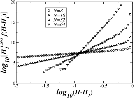
Figure 1: Logarithmic plot of the rescaled distribution $H_{1}^{1-N/2}f(H-H_{1})$ as a function of the transformed variable $H-H_{1}$ for $N=8$ (circles), $16$ (triangles up), $32$ (squares), and $64$ (triangles down) anharmonic oscillators. The solid straight lines are the best fit to the simulation data of the expected power-law behavior Eq. (14). The slopes are 1.0068 (1.0), 3.07 (3.0), 7.21 (7.0), and 15.27 (15.0) for $N=8$, $16$, $32$, and $64$, respectively, and the numbers in parentheses indicate the expected values obtained from Eq. (15). The departure from the power-law behavior at the extremes of the curves is due to finite-time sampling.

In Fig. 1 we show the logarithmic plot of the distribution $f({\bf p}_{1},{\bf p}_{2},\ldots)$ against the transformed variable $H-H_{1}$ for systems with $N=8$, $16$, $32$, and $64$ oscillators. Based on the above result, we assume ergodicity and compute the distribution of momenta from the fluctuations in time of $H_{1}$ through the relation

$$f(H_{1})\propto H_{1}^{(N/2)-1}f({\bf p}_{1},{\bf p}_{2},\ldots),$$ (20)

where the $H_{1}^{(N/2)-1}$ factor accounts for the degeneracy of the momenta consistent with the magnitude of $H_{1}$ (cf. khinchin ). Indeed, we observe in all cases that the fluctuations in $H_{1}$ follow very closely the prescribed power-law behavior Eq. (14), with exponents given by Eq. (15). These results, therefore, provide clear evidence for the validity of our dynamical approach to the generalized thermostatistics.

IV Conclusion

In conclusion, we have shown that the generalized formalism of Tsallis can be applied to homogeneous Hamiltonian systems to engender an adequate theoretical framework for the statistical mechanics of finite systems. Of course, we do not expect that our approach can explain the whole spectrum of problems in which Tsallis statistics can be applied. However, our exact results clearly indicate that, as far as homogeneous Hamiltonian systems are concerned, the range of the interacting potential should play no role in the equilibrium statistical properties of a system in the thermodynamic limit inhomog . Under these conditions, the conventional BG thermostatistics remains valid and general, i.e., for the specific class of homogeneous Hamiltonians investigated here, the thermodynamic limit ($N\to\infty$) leads always to BG distributions.

- (1) C. Tsallis, J. Stat. Phys. 52, 479 (1988).
- (2) C. Tsallis, “Nonextensive statistical mechanics and thermodynamics: Historical background and present status,” in Nonextensive Statistical Mechanics and its Applications, S. Abe and Y. Okamoto (Eds.) (Springer-Verlag, Berlin, 2001); also in Braz. J. Phys. 29, 1 (1999).
- (3) See http://tsallis.cat.cbpf.br/biblio.htm for an updated bibliography.
- (4) A. R. Plastino and A. Plastino, Phys. Lett. A 193, 140 (1994).
- (5) S. Abe and A. K. Rajagopal, Phys. Lett. A 272, 341 (2000); J. Phys. A 33, 8733 (2000).
- (6) G. Wilk and Z. Wlodarczyk, Phys. Rev. Lett. 84, 2770 (2000).
- (7) J. D. Ramshaw, Phys. Lett. A 198, 122 (1995).
- (8) E. Vives and A. Planes, Phys. Rev. Lett. 88, 020601 (2002).
- (9) M. P. Almeida, Physica A 300, 424 (2001).
- (10) Observing that , where is the structure function of the heat bath, and is its derivative, and integrating Eq. (3) with the initial condition we get that , where is a constant. This implies that the structure function is a finite power of for , and therefore the phase space is finite dimensional.
- (11) It is worth mentioning that a related connection between scale-invariant thermodynamics and Tsallis statistics was also proposed by P. A. Alemany, Phys. Lett. A, 235 452 (1997), although the approach adopted by the author is not based on the more fundamental ergodic arguments presented here.
- (12) L. D. Landau and E. M. Lifshitz, Mechanics, 3rd. Ed. (Reed Educ. and Prof. Pub., 1981). In this reference, “scale invariance” is under the name of “mechanical similarity”.
- (13) J. S. Andrade Jr., M. P. Almeida, A. A. Moreira and G. A. Farias, Phys. Rev. E 65, 036121 (2002).
- (14) A. I. Khinchin, Mathematical Foundations of Statistical Mechanics (Dover, New York, 1949).
- (15) B. P. Vollmayr-Lee and E. Luijten, Phys. Rev. Lett. 85, 470 (2000).
- (16) R. Salazar and R. Toral, Phys. Rev. Lett. 83, 4233 (1999).
- (17) B. P. Vollmayr-Lee and E. Luijten, Phys. Rev. E 63, 031108 (2001).
- (18) V. Latora, A. Rapisarda and C. Tsallis, Phys. Rev. E 64, 056134 (2001).
- (19) E. Fermi, J. Pasta, S. Ulam and M. Tsingou, Studies of nonlinear problems I. Los Alamos preprint LA-1940 (7 November 1955); Reprinted in E. Fermi, Collected Papers, Vol. II (Univ. of Chicago Press, Chicago, 1965) p. 978.
- (20) J. Ford, Phys. Rep. 213, 271 (1992).
- (21) V. L. Berdichevsky, Thermodynamics of Chaos and Order (Addison Wesley, 1997).
- (22) V. M. Bannur, P. K. Kaw and J. C. Parikh, Phys. Rev. E 55, 2525 (1997).
- (23) For recent investigations on the inhomogeneous case, see e.g. C. Tsallis, Physica A 302, 187 (2001), and V. Latora, A. Rapisarda, and C. Tsallis, Phys. Rev. E 64, 056134 (2001).