Ab initio quasiharmonic equations of state
for dynamically-stabilized soft-mode materials

Abstract

We introduce a method for treating soft modes within the analytical framework of the quasiharmonic equation of state. The corresponding double-well energy-displacement relation is fitted to a functional form that is harmonic in both the low- and high-energy limits. Using density-functional calculations and statistical physics, we apply the quasiharmonic methodology to solid periclase (MgO). We predict the existence of a B1–B2 phase transition at high pressures and temperatures.

61.50.Ks, 64.70.Kb, 71.20.-b

I Introduction

The quasiharmonic approximation [1] provides a means of extracting finite-temperature properties of materials from static calculations. It assumes the vibrational properties can be understood in terms of excitations of non-interacting harmonic normal modes: phonons. Lattice dynamics [2] can be used to calculate phonon energies by evaluating the eigenvalues of the dynamical matrix, which involves second derivatives of the crystal energy with respect to atomic displacements.

The frequencies of these modes depend on the crystal’s density. Hence they have a temperature-dependence that arises simply because of thermal expansion in the material.

Recent developments in ab initio energy calculations have enabled full phonon dispersion curves to be obtained, leading to a resurgence of interest in the quasiharmonic approach. Difficulties arise, however, when the dynamical matrix has negative eigenvalues, indicating that the crystallographic structure is not a local minimum of energy. Such crystals may be dynamically stabilized: because of their large entropy, they may represent a minimum of free energy at high temperature. Within the conventional assumption of harmonic phonons, the quasiharmonic framework leads to divergent free energies in these cases. Such systems have been treated numerically from first principles using Monte Carlo methods with effective Hamiltonians [3] or molecular dynamics simulations of a reduced set of modes [4]. Here, we relax the quasiharmonic assumption of harmonic modes while retaining the approximation of non-interacting phonons and show how the intrinsic anharmonicity of such modes can be included in analytic free energy calculations.

The mineral periclase (MgO) is of some geological significance as one of the supposed constituents of the Earth’s lower mantle. It is generally believed that along the geotherm—the conditions of pressure and temperature actually occurring in the mantle—periclase remains in a single phase. Under other conditions, however, previous calculations have suggested that periclase has two phases in its solid state: a sodium chloride-like face-centered cubic phase (B1) and a cesium chloride-like simple cubic phase (B2) that is favored at extremely high pressures [5].

Imaginary phonon frequencies are found in the B2 phase of periclase and have attracted enormous attention in the other principal constituent of the lower mantle, magnesium silicate perovskite (MgSiO₃) [6, 7, 8, 9, 10].

Equilibrium structures, thermodynamic properties and compositions depend on the free energy. Here we present a calculation of the free energy of periclase as a function of density and temperature. We use the pseudopotential-plane wave approach to evaluate total energies and the method of finite displacements to evaluate pressure-dependent force constants [11], including effective charges and dielectric constants [12] for the longitudinal optic modes. Based on calculated phonon frequencies and the quasiharmonic approximation, we present a first-principles calculation of the phase diagram and thermodynamic equation of state of solid periclase: the relationship between pressure, density and temperature.

II The quasiharmonic method

A Ab initio calculation of specific Helmholtz free energies

The first stage of the calculation is to obtain the specific (with respect to mass) Helmholtz free energy of each phase as a function of density and temperature. We write the free energy as the sum of the frozen-ion interaction energy and the free energy due to lattice vibrations.

1 The frozen-ion energy

The frozen-ion energy—the interaction energy of the crystal with the ions fixed in their equilibrium positions—is, by definition, temperature-independent. Hence the free energy is simply equal to the internal energy. In order to determine the dependence on density, total energy densiyty functional calculations are carried out for each phase at a range of different lattice parameters.

2 The lattice thermal Helmholtz free energy

We calculate the lattice thermal Helmholtz free energy of each phase as a function of density and temperature within the framework of the harmonic approximation [13].

For a range of lattice parameters, we evaluate the matrix of force constants for a supercell (several unit cells) of the phase under consideration, subject to periodic boundary conditions. We evaluate the forces on the ions in a crystal when one ion is displaced slightly from its equilibrium position: from such calculations the matrix of force constants may be constructed[11].

We denote the matrix of force constants by $\phi$, where $\phi_{l,n,\alpha;m,p,\beta}$ is the component of force in direction $\alpha$ on ion $n$ in unit cell $l$ when ion $p$ in unit cell $m$ is displaced infinitesimally in direction $\beta$, divided by the magnitude of the displacement.

Pairs of density-functional calculations are carried out with an ion displaced from equilibrium along one of the Cartesian axes by a small amount in first a positive and then a negative sense. By averaging the resulting Hellmann-Feynman forces on the ions from the first simulation with the negative of the forces from the second, first-order anharmonic contributions to the force constants are eliminated.

The set of rotations under which the crystal structure is invariant are identified and the rotation matrices, together with the mappings between the ions under the symmetry operations, are evaluated. For a given pair of ions $(l,n)$ and $(m,p)$, the matrix of force constants $\phi_{l,n,\alpha;m,p,\beta}$ transforms as a second-rank tensor. However, for a symmetry operation, the transformed matrix must be the same as the (unrotated) matrix of force constants between the pair of ions which are mapped to $(l,n)$ and $(m,p)$. Hence, new elements of the matrix of force constants can be obtained by application of these point symmetries. Translational symmetries can be identified and exploited in a similar fashion.

The matrix of force constants should be symmetric [13] and Newton’s third law must be satisfied: if an ion is displaced slightly then the restoring force on that ion must be equal and opposite to the total force on all of the other ions. Hence we must have:

$$\phi_{l,n,\alpha;m,p,\beta} = \phi_{m,p,\beta;l,n,\alpha}$$ (1)

$$\phi_{l,n,\alpha;l,n,\beta} = -\sum_{(m,p)\neq(l,n)}\phi_{l,n,\alpha;m,p,\beta}.$$ (2)

The force constants are obtained from separate numerical calculations; hence small violations of these requirements may occur. These two conditions are therefore alternately imposed on the matrix of force constants until further application leaves the matrix unchanged [11].

The next stage of the calculation involves the construction of dynamical matrices [13] for various wavevectors in the first Brillouin zone. Diagonalization of the dynamical matrix for a given wavevector gives the spectrum of corresponding eigenfrequencies. Strictly, these are only exact when the wavelengths are commensurate with the dimensions of the supercell [11]. However, provided that the resulting dispersion curves are smooth, it may be assumed that the interpolation errors are negligible.

Cochran and Cowley [14] have shown that the elements of the dynamical matrix for an ionic crystal can be written as the sum of a term that behaves analytically as the wavevector tends to zero and a term that is non-analytic at the zone center. The latter term vanishes as the boundary of the Brillouin zone is approached. This term arises because longitudinal optic (LO) phonons cause an electric polarization field to be set up within the crystal as the oppositely-charged ions are displaced in opposite directions. The resulting long-range interactions cannot be calculated within the framework we have described so far because of the limited size of the simulation supercell. At the zone center itself, the LO phonon sets up a uniform electric polarization that is incompatible with the periodic boundary conditions on the supercell.

Cochran and Cowley’s expression for the dynamical matrix is:

$$\tilde{\phi}_{n,\alpha;p,\beta}({\bf k})= \tilde{\phi}^{N}_{n,\alpha;p,\beta}({\bf k})+\frac{4\pi e^{2}}{\Omega|{\bf k}|^{2}\sqrt{M_{n}M_{p}}}$$ (3)

$$\times \left(\sum_{\gamma=1}^{3}k_{\gamma}Z_{n,\gamma,\alpha}({\bf k})\right)^{\ast}\epsilon_{0}^{-1}({\bf k})$$ (4)

$$\times \left(\sum_{\gamma=1}^{3}k_{\gamma}Z_{p,\gamma,\beta}({\bf k})\right),$$ (5)

where ${\bf k}$ is the wavevector, $e$ is the electronic charge, $\Omega$ is the volume of the unit cell, $M_{n}$ is the mass of ion $n$, $Z_{n,\alpha,\beta}({\bf k})$ is the Born effective charge tensor for ion $n$ and $\epsilon_{0}({\bf k})$ is the electronic (frequency dependent) dielectric function. The first term on the right-hand side is the component of the dynamical matrix that is analytic as ${\bf k}\to 0$, while the second term is the non-analytic part due to macroscopic polarization effects. We use our matrix of force constants evaluated using the Hellmann-Feynman theorem in a cubic supercell to evaluate the analytic part as:

$$\tilde{\phi}^{N}_{n,\alpha;p,\beta}({\bf k})=\frac{1}{\sqrt{M_{n}M_{p}}}\sum_{m}\phi_{0,n,\alpha;m,p,\beta}e^{-i{\bf k}\cdot({\bf R}_{0}-{\bf R}_{m})},$$ (6)

where ${\bf R}_{m}$ is the position vector of unit cell $m$.

Following Parlinski et al[12] we assume that the second term on the right-hand side of Equation 5 falls off from its value at the Brillouin zone center with a Gaussian profile. For wavevectors in the first Brillouin zone this term is:

$$\frac{4\pi e^{2}}{\Omega|{\bf k}|^{2}\sqrt{M_{n}M_{p}}\epsilon_{0}({\bf 0})}\left(\sum_{\gamma=1}^{3}k_{\gamma}Z_{n,\gamma,\alpha}({\bf 0})\right)^{\ast}$$ (7)

$$\times \left(\sum_{\gamma=1}^{3}k_{\gamma}Z_{p,\gamma,\beta}({\bf 0})\right)\times e^{-\left(\frac{|{\bf k}|}{\rho_{0}\kappa^{1/2}}\right)^{2}},$$ (8)

where $\kappa^{1/2}$ is the distance from the center to the boundary of the Brillouin zone along the $k_{x}$-, $k_{y}$- and $k_{z}$-directions and $\rho_{0}$ is a parameter determining the rate at which the term falls off as the edge of the Brillouin zone is approached. Following Parlinski, we set $\rho_{0}\equiv 1.2$.

The frequency density-of-states function is evaluated using the method of Swift [15] in which the Brillouin zone is sampled using Monte Carlo methods. For a single harmonic mode of frequency $\omega$, the Helmholtz free energy is given by:

$$F_{1}(\omega)=k_{B}T\log\left(e^{\beta\hbar\omega/2}-e^{-\beta\hbar\omega/2}\right),$$ (9)

where $\hbar$ is the Dirac constant, $k_{B}$ is Boltzmann’s constant, $T$ is the temperature and $\beta=1/k_{B}T$. Hence, by numerically integrating the product of the specific density-of-states with the mean free energy of a normal mode, the specific lattice thermal free energy can be calculated for a range of temperatures. The dependence on density is found by interpolating between the results at different lattice parameters.

B Polymorphism

C The Gibbs free energy

We have calculated the Helmholtz free energy $f(v,T)$ as a function of temperature $T$ and specific volume $v$ (the reciprocal of the density). However, the appropriate thermodynamic potential for constructing the $(p,T)$-phase diagram and evaluating the polymorphic equation of state is the specific Gibbs free energy $g(p,T)$, where $p$ is the pressure. The Gibbs free energy function for each phase can be evaluated using the Legendre transformation:

$$g(p,T)=f+pv=f-\left(\frac{\partial f}{\partial v}\right)_{T}v.$$ (10)

D The phase diagram

Under conditions of fixed pressure and temperature, the system consists entirely of the available phase with the lowest Gibbs free energy. Thus the phase diagram in $(p,T)$-space can be evaluated.

E Combining phases

For each pressure and temperature, we may evaluate the polymorphic Gibbs free energy $g_{\rm poly}(p,T)$ as the lowest of the Gibbs free energies for each phase. Given this, we may carry out a Legendre transformation to the polymorphic Helmholtz free energy:

$$f_{\rm poly}(v,T)=g_{\rm poly}-pv=g_{\rm poly}-p\left(\frac{\partial g_{\rm poly}}{\partial p}\right)_{T}.$$ (11)

Differentiating this, we obtain the pressure as a function of specific volume and temperature: the desired polymorphic equation of state.

III Extension of the quasiharmonic method to unstable phonons

A Analytic model of soft-mode phonons

In minerals such as perovskites [7] it is possible to describe the transition from a high-temperature phase to a low-temperature phase of lesser symmetry as the “freezing in” of a finite amplitude of an unstable phonon of the high-symmetry phase, plus a finite strain on the unit cell. We consider the application of quasiharmonic ideas to these materials.

The simple harmonic model gives a negative energy and divergent free energy arising from the unstable modes. In reality, the soft-mode phonon is best described by a potential double-well with a local maximum at the mean structure, corresponding to the high-symmetry phase.

Let $x_{i}$ be a coordinate describing the structural feature involved in the phase transition at a particular wavevector. The corresponding normal mode can be modeled by considering the dynamics of the set of $\{x_{i}\}$ moving in fixed local potential double-wells [16]. In the harmonic limit, normal modes are uncoupled. However, because we are considering finite displacements there will in general be coupling between our double-well oscillators, this being most pronounced around the phase transition and at high temperatures. Coupling can be approximately treated by renormalization [16].

Much work has been concentrated on the Landau model in which the double-well is a free energy in the form of a quartic polynomial $V(x)=Ax^{4}-B(T)x^{2}$, where $B(T)$ changes sign with temperature through coupling to other modes.

Such a polynomial expansion of the total energy is also possible, perhaps incorporating still higher-order terms [3]. However, analytic terms beyond second order imply phonon coupling. This is inconsistent with the harmonic approximation used to describe non-soft modes: even at high phonon number the normal modes are assumed to be harmonic and therefore independent of each other.

We propose instead to describe the entire soft-phonon branch via a double-well of form:

$$V(x)=\frac{1}{2}m\omega_{0}^{2}x^{2}+\epsilon(e^{-x^{2}/2\sigma^{2}}-1).$$ (12)

where $\epsilon$, $\omega_{0}$ and $\sigma$ are wavevector dependent. Provided that $\epsilon>m\omega_{0}^{2}\sigma^{2}$, there are minima at:

$$x=x_{\pm}\equiv\pm\sqrt{2\sigma^{2}\log(\epsilon/m\omega_{0}^{2}\sigma^{2})},$$ (13)

separated by a barrier of height:

$$\Delta V \equiv V(0)-V(x_{\pm})$$ (14)

$$= \epsilon-m\omega_{0}^{2}\sigma^{2}\left(1+\log\left(\epsilon/m\omega_{0}^{2}\sigma^{2}\right)\right).$$ (15)

This form of potential has the advantage of being approximately quadratic in both the low-energy and high-energy limits. Specifically, for the low-energy case at $x=x_{\pm}$, we have:

$$\frac{d^{2}V}{dx^{2}}=2m\omega_{0}^{2}\log\left(\epsilon/m\omega_{0}^{2}\sigma^{2}\right),$$ (16)

which is equivalent to an harmonic oscillator of frequency:

$$\omega_{0}^{\prime}=\sqrt{2\omega_{0}^{2}\log(\epsilon/m\omega_{0}^{2}\sigma^{2})}.$$ (17)

On the other hand, for the high-energy case, the potential approximates that of an harmonic oscillator of frequency $\omega_{0}$.

Soft modes do not usually show abnormal dependence on temperature—except in the vicinity of the phase transition. Therefore we expect our model to be more widely applicable than models where soft modes are treated as quartic and other modes as harmonic.

The (imaginary) harmonic frequency $\omega_{c}$ about the (unstable) center of the well is given by:

$$\omega_{c}^{2}=\omega_{0}^{2}-\frac{\epsilon}{m\sigma^{2}}.$$ (18)

B Isolated double-well oscillators

We now consider the problem of motion in an isolated potential double-well.

1 Classical solution

To evaluate the mechanical energy, we assume the mode is in thermal contact with a heat bath at the appropriate temperature. The mean energy is given by:

$$\langle E\rangle = \frac{\int_{-\infty}^{\infty}\int_{-\infty}^{\infty}H(p,x)e^{-\beta H(p,x)}\,dp\,dx}{\int_{-\infty}^{\infty}\int_{-\infty}^{\infty}e^{-\beta H(p,x)}\,dp\,dx}$$ (19)

$$= \frac{k_{B}T}{2}+\frac{\int_{0}^{\infty}V(\sigma z)e^{-\beta V(\sigma z)}\,dz}{\int_{0}^{\infty}e^{-\beta V(\sigma z)}\,dz},$$ (20)

where $H(p,x)=p^{2}/2m+V(x)$ is the Hamiltonian of the isolated mode as a function of $x$ and $p$, the canonical momentum conjugate to $x$. $\beta=1/k_{B}T$ where $k_{B}$ is Boltzmann’s constant and $T$ is the temperature.

For a given energy $E$, the frequency of our isolated mode can be evaluated using the action-angle method. The action variable is:

$$j\equiv\frac{1}{2\pi}\oint p\,dx.$$ (21)

If the mode has energy $E\geq\epsilon$, so that there is sufficient energy to cross the barrier each libration, we find that:

$$j=\frac{2\sigma}{\pi}\int_{0}^{x_{M}(E)/\sigma}\sqrt{2mE-m^{2}\omega_{0}^{2}\sigma^{2}z^{2}-2m\epsilon e^{-z^{2}/2}}\,dz,$$ (22)

where $x_{M}$ is the positive solution of $V(x)=E$. On the other hand, if $E<\epsilon$, so that the motion is confined to one side of the double-well, we find that:

$$j=\frac{\sigma}{\pi}\int_{x_{m}(E)/\sigma}^{x_{M}(E)/\sigma}\sqrt{2mE-m^{2}\omega_{0}^{2}\sigma^{2}z^{2}-2m\epsilon e^{-z^{2}/2}}\,dz,$$ (23)

where $x_{M}$ is the greater of the two positive solutions and $x_{m}$ is the lesser.

In either case, the corresponding frequency $\omega$ may be evaluated using Equation 24:

$$\frac{1}{\omega}=\frac{\partial j}{\partial E}.$$ (24)

Taken together, the results of Equations 20, 22, 23 and 24 allow us to calculate numerically the frequency of an isolated oscillator moving with the mean thermal energy as a function of temperature. Example results are shown in Figure 1. Typical “soft-mode” behavior is observed, with the frequency dropping to zero in a cusp at the transition temperature. This simple approach was used in early studies of MgSiO₃ [17].

2 Quantum solution

The energy eigenfunctions of a particle moving in a symmetric potential must be either symmetric or antisymmetric. Furthermore, by considering building up the Gaussian barrier adiabatically, it is clear that the symmetry of the eigenfunctions must be the same as for those of the harmonic oscillator.

The definite symmetry of the wavefunctions leads to a “paradox” for wells of finite separation. If we know the energy of the oscillator then it is in an energy eigenstate and the wavefunction is either symmetric or antisymmetric. Hence the probability distribution is symmetric about the center of the double-well and we cannot meaningfully say which side the oscillator is confined in, even if its energy is much less than the barrier height. Thus it is not conceptually clear that equating the mean thermal energy with the barrier height gives the correct transition temperature. We discuss this further in Section III D.

The Hamiltonian operator for a particle moving in the quadratic potential without the additional Gaussian potential is:

$$\hat{H}^{0}=-\frac{\hbar^{2}}{2m}\frac{\partial^{2}}{\partial x^{2}}+\frac{1}{2}m\omega_{0}^{2}x^{2}.$$ (25)

The well-known energy eigenvalues and eigenfunctions for the time-independent Schrödinger equation $\hat{H}^{0}\phi_{n}=E^{0}_{n}\phi_{n}$ are:

$$E^{0}_{n}=(n+1/2)\hbar\omega_{0}$$ (26)

and

$$\phi_{n}=\frac{2^{-n/2}}{\sqrt{n!}}\left(\frac{m\omega_{0}}{\hbar\pi}\right)^{1/4}e^{-m\omega_{0}x^{2}/2\hbar}H_{n}\left(\sqrt{\frac{m\omega_{0}}{\hbar}}x\right)$$ (27)

for $n\in\mathcal{N}_{0}$, where $H_{n}(x)$ is the $n$th Hermite polynomial.

The Hamiltonian operator for a particle moving in the double-well is $\hat{H}=\hat{H}^{0}+V_{1}$ where $V_{1}=\epsilon(e^{-x^{2}/2\sigma^{2}}-1)$ is the extra Gaussian term. Let the eigenfunctions and eigenenergies of the full Hamiltonian be $\psi_{n}$ and $E_{n}$.

The eigenfunctions of the simple harmonic oscillator (SHO) are chosen as the basis of wavefunction space. This choice makes the computation particularly simple, as will be seen below.

The matrix elements of the Hamiltonian with respect to our chosen basis are:

$$\langle\phi_{i}|\hat{H}\phi_{j}\rangle = \langle\phi_{i}|\hat{H}^{0}\phi_{j}\rangle+\langle\phi_{i}|V_{1}\phi_{j}\rangle$$ (28)

$$= (i+1/2)\hbar\omega_{0}\delta_{i,j}$$ (30)

$$+\frac{\epsilon}{2^{(i+j)/2}\sqrt{i!j!\pi}}\int_{-\infty}^{\infty}e^{-Kz^{2}}H_{i}(z)H_{j}(z)\,dz,$$

where $K\equiv\hbar/2m\omega_{0}\sigma^{2}+1$. Note that the matrix is real and symmetric.

The Hermite polynomials satisfy $H_{i}(-x)=(-1)^{i}H_{i}(x)$, so that $\langle\phi_{i}|V_{1}\phi_{j}\rangle=0$ if $i+j$ is odd. If $i+j$ is even then the integrand is an even function. Hence, in this case:

$$\langle\phi_{i}|V_{1}\phi_{j}\rangle=\frac{2\epsilon}{2^{(i+j)/2}\sqrt{i!j!\pi}}\int_{0}^{\infty}e^{-Kz^{2}}H_{i}(z)H_{j}(z)\,dz.$$ (32)

The eigenvalues of the matrix of the Hamiltonian are the allowed energy levels. For energies that are large compared with the barrier height the particle will spend most of its time away from the center of the well; hence we expect that the system will behave as a SHO in this limit. Indeed, it is clear from Equation 32 that the elements of the matrix $\langle\phi_{i}|V_{1}\phi_{j}\rangle$ fall off rapidly as $i$ and $j$ increase. Hence, for large $i$ or $j$, the eigenvalues of the Hamiltonian tend to to those of the SHO. Thus we only need to diagonalize the upper left-hand corner (say, the $(n_{c}+1)\times(n_{c}+1)$ submatrix) in order to obtain the first $n_{c}+1$ energy levels $E_{0}$ to $E_{n_{c}}$. Beyond $n_{c}$ the eigenvalues may be taken to be those of the SHO. The comparative ease with which the Hamiltonian matrix can be diagonalized is one of the advantages of the quadratic-plus-gaussian double-well over the quartic double-well potential, although there is no analytic form equivalent to equation 9

Assuming that $n_{c}$ is sufficiently large, the canonical partition function can be written as:

$$Z = \sum_{n=0}^{n_{c}}e^{-\beta E_{n}}+\sum_{n=n_{c}+1}^{\infty}e^{-\beta(n+1/2)\hbar\omega_{0}}$$ (33)

$$= \sum_{n=0}^{n_{c}}e^{-\beta E_{n}}+\frac{e^{-\beta\hbar\omega_{0}(n_{c}+1)}}{e^{\beta\hbar\omega_{0}/2}-e^{-\beta\hbar\omega_{0}/2}}.$$ (34)

The free energy of the double-well oscillator can then be evaluated as:

$$F_{1}=-k_{B}T\log\left(Z\right).$$ (35)

C Practical implementation in the quasiharmonic method

Having proposed that each soft mode at a given wavevector be described by a double-well of the form given in Equation 12, we now describe how the parameters $\epsilon$, $\sigma$ and $\omega_{0}$ can be determined. Note that if the $\{x_{i}\}$ are mass-reduced phonon coefficients then we may, without loss of generality, set $m=1$.

Consider the phonon dispersion curve of a crystal structure in which imaginary frequencies are present. Those branches that remain real throughout the whole of the Brillouin zone are treated as harmonic and, for each mode at each wavevector, Equation 9 may be used to find the corresponding free energy. For those branches that are imaginary in some region of the Brillouin zone, however, we propose the following treatment:

1. At each symmetry point of the Brillouin zone the eigenvector corresponding to the relevant mode should be evaluated and the displacement pattern frozen into the crystal. Ab initio techniques can then be used to find the corresponding low-symmetry structure, if desired. Using three total energy calculations with different amplitudes of the soft phonon frozen into the structure, we may evaluate the parameters $\epsilon$, $\sigma$ and $\omega_{0}$ of the double-well. Note that it is possible to fit equation 12 to every branch even if the mode is not imaginary since that Equation 12 does not necessarily describe a double-well. In practice the harmonic approximation is used for all-real branches, it is equivalent to setting $\epsilon=0$.

2. For each branch we use our results for the double-well parameters at the symmetry points to construct interpolating polynomials over the whole of the Brillouin zone for the $\epsilon$ and $\sigma$ parameters.

3. For any wavevector in the Brillouin zone, we may find the spectrum of corresponding (possibly imaginary) frequencies. Provided we know to which branch these modes belong, we have sufficient information to determine the parameters of the appropriate double-well for each mode. $\epsilon$ and $\sigma$ are found by interpolating to our wavevector and the unstable frequency gives $\omega_{c}$ (see Equation 18), from which we may find $\omega_{0}^{2}=\omega_{c}^{2}+\epsilon/m\sigma^{2}$.

4. Hence, for any given wavevector, the free energy of each mode, whether harmonic or soft, can be evaluated. These free energies can be summed to give the free energy contribution from all modes at the given wavevector.

5. The free energy can then be integrated over all wavevectors in the Brillouin zone to give the total lattice thermal free energy. By using a grid-based scheme to integrate over an irreducible wedge of the zone and by making use of the continuity of the gradient of each branch, it is possible to keep track of which branch is which—necessary if the appropriate values of $\epsilon$ and $\sigma$ are to be interpolated in the pressence of imaginary branch crossings. The problem of interpolation over an irreducible wedge of the Brillouin zone has been studied extensively in the context of electronic eigenvalues: see, for example, Reference [18].

The high-symmetry dynamically stabilized phase and the low-symmetry “frozen-phonon” phase can now be treated as being distinct. Hence the methodology of Section II B can be applied to find the phase diagram.

D Interpretation of the soft mode transition

Consider an isolated symmetric double-well oscillator. For the probability density to be asymmetric—necessary if we are to meaningfully say that the particle is in one well or the other—we must have a mixture of symmetric and antisymmetric energy eigenstates. Therefore we cannot simultaneously know the energy of our particle and which well it is in unless we break the symmetry (e.g. by allowing the crystal to distort under phonon-strain coupling).

If the oscillating particle’s wavefunction is a superposition of different energy eigenfunctions then the expansion coefficients will evolve in time (provided the system remains both undisturbed and unobserved) according to the Schrödinger equation. Hence the quantum mechanical expectation value of the particle’s position, $\langle x\rangle$ changes in time.

The time-dependent wavefunction can be written as:

$$\Psi(x,t)=\sum_{n=0}^{\infty}c_{n}e^{-iE_{n}t/\hbar}\psi_{n}(x).$$ (36)

Hence the expectation of $x$ can be written as:

$$\langle x\rangle = \sum_{n=0}^{\infty}\sum_{m=0}^{\infty}c_{n}^{\ast}c_{m}e^{i(E_{n}-E_{m})t/\hbar}\langle\psi_{n}|x\psi_{m}\rangle$$ (37)

$$= 2\sum_{n\,{\rm even}}\sum_{m\,{\rm odd}}\left|c_{n}\right|\left|c_{m}\right|$$ (39)

$$\hskip 51.21504pt\times\cos(\omega_{nm}t+\eta_{nm})\langle\psi_{n}|x\psi_{m}\rangle$$

where $\omega_{nm}=|E_{n}-E_{m}|/\hbar$ and $\eta_{nm}=(\arg(c_{m})-\arg(c_{n})){\rm sgn}(\omega_{nm})$. Note that we use the fact that $\langle\psi_{n}|x\psi_{m}\rangle=0$ if $\psi_{n}$ and $\psi_{m}$ are either both odd or both even since $x$ itself is odd. We also use the fact that $\langle\psi_{n}|x\psi_{m}\rangle=\langle\psi_{m}|x\psi_{n}\rangle$.

We assume that the energy levels are initially populated according to Boltzmann statistics; thus $|c_{n}|^{2}=Z^{-1}e^{-\beta E_{n}}$, where $\beta=1/k_{B}T$ and $Z=\sum_{n=0}^{\infty}e^{-\beta E_{n}}$ is the canonical partition function.

So we have:

$$\langle x\rangle=\sum_{n\,{\rm even}}\sum_{m\,{\rm odd}}\Gamma_{nm}\cos(\omega_{nm}t+\eta_{nm}),$$ (40)

where $\Gamma_{nm}=2Z^{-1}e^{-\beta(E_{n}+E_{m})/2}\langle\psi_{n}|x\psi_{m}\rangle$ is the amplitude of the sinusoidal component in the expansion of $\langle x\rangle$ with frequency $\omega_{nm}$.

For the harmonic oscillator potential, the frequencies of the oscillations in $\langle x\rangle$ are of the form $\omega_{nm}=|E_{n}-E_{m}|/\hbar=|n-m|\omega_{0}$. Thus the lowest oscillation frequency is $\omega_{0}$. For the symmetric double-well, however, we end up with a set of pairs of energy levels that are very close to each other (becoming degenerate in the limit that the barrier height goes to infinity). These give rise to oscillation frequencies very much lower than $\omega_{0}$.

As the temperature is increased, higher frequency components have larger $\Gamma$ coefficients. We suggest that the soft mode phase transition be judged to occur when the frequency with the highest coefficient exceeds the frequency of the experimental probe. When this has happened, the predominant sinusoidal component of $\langle x\rangle$ has a frequency higher than can be measured by the experimental probe, and so it appears to the experimenter that $\langle x\rangle=0$. Below this temperature, measurements of $\langle x\rangle$ will tend to find it in one well or the other. This definition is different from the polymorphic one (Section II B) because of the contribution to the free energy from the symmetry-breaking distortion of the lattice that inevitably accompanies the transition. In particular, the quasiharmonic transition is first-order while this measurement dependent “soft mode” one is second-order [16].

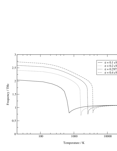
FIG. 1.: Classical frequency of a double-well oscillator in thermal contact with a heat bath plotted against temperature for various barrier heights $\epsilon$. The other double-well parameters are: $m=1$, $\omega_{0}=0.0691$ eV^1/2 Å^-1 amu^-1/2 and $\sigma=1.866$ amu^1/2Å. The frequency falls to zero in a cusp at the phase transition. At $\epsilon=0.2972$ eV, the double-well parameters are appropriate for the double-well describing the orthorhombic–tetragonal transition in MgSiO₃ at zero pressure [7]. Thus this model predicts a soft mode transition temperature of 2609 K, if the coupling of the soft phonon to strain is neglected.

Thus the first-order transition is determined by comparing:

1. The free energy of the soft-mode phase, calculated as above, expanded about an unstable frozen-ion structure without strain-phonon coupling.

   with

2. The free energy of the low symmetry phase, calculated by expanding about the minimum of total energy.

Typically, the former will have higher entropy (sampling from both wells) while the latter has lower energy.

E Absorption of low-frequency photons

Figure 2 shows the energy difference between neighboring energy levels $(E_{n}-E_{n-1})/\hbar$ plotted against the mean of the two energies $(E_{n}+E_{n-1})/2$ for the quantum double-well oscillator. Absorption of photons at frequency $(E_{n}-E_{n-1})/\hbar$ is symmetry-allowed.

For energies in excess of the barrier height the frequency $(E_{n}-E_{n-1})/\hbar$ is virtually identical to the classical frequency for energy $(E_{n}+E_{n-1})/2$, obtained using the method of Section III B 1. In the very high-energy limit the frequency behaves as that of the quadratic potential well without the Gaussian barrier.

For energies less than the barrier height the energy levels tend to degenerate pairs of levels. The frequencies given by the difference between the energy levels of neighboring pairs again correspond to the classical frequencies. However, the pairs of almost-degenerate eigenstates imply the existence of very low-frequency absorption peaks. (These are the very low frequencies that alternate with the classical frequencies below the transition energy in Figure 2.) It should be noted that these frequencies are not associated with the normal modes of the low-symmetry phase and do not, therefore, contribute to the quasiharmonic thermal energy. They are a feature of the quantum double-well oscillator without classical analog.

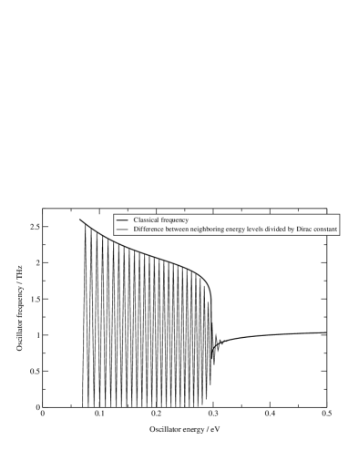
FIG. 2.: Thick line: Frequency of classical isolated double-well oscillator against energy. The double-well parameters are as for Figure 1 with $\epsilon=0.2972$ eV. Fine line: Energy differences $(E_{i}-E_{i-1})/\hbar$ against energy $(E_{i}+E_{i-1})/2\hbar$ for quantum oscillator.

IV Application of quasiharmonic methods to periclase

A Computational details

1 The cold-curve

For each lattice parameter the total energy is evaluated using the CASTEP software package [19], which utilizes density-functional theory in the generalized gradient approximation (GGA) [20]. The ionic cores are accounted for using ultrasoft pseudopotentials [21] in Kleinman-Bylander form [22]. The wavefunctions of the valence electrons are expanded in a plane wave basis set up to an energy cutoff of 540 eV.

For the B1 phase, the simulation cell consists of a single cubic unit cell. The Brillouin zone is sampled at 20 special points generated from an $8\times 8\times 8$ mesh using the Monkhorst-Pack scheme [23]. For the B2 phase, the simulation cell is a single cubic primitive cell. The Brillouin zone is sampled at 35 special points from a $9\times 9\times 9$ mesh. In each case the point symmetries of the crystal are enforced [24].

The equilibrium lattice parameter of the B1 phase at zero external pressure (which corresponds to the minimum of the cold-curve) calculated using CASTEP is $a=4.259$ Å, which may be compared with an experimentally determined parameter $a=4.2115(1)$ Å [28]. The difference between the theoretical and experimental values is about 1%.

2 Determination of the matrix of force constants

The supercells simulated to determine the matrices of force constants for the B1 phase consist of $2\times 2\times 2$ cubic unit cells (64 atoms). Thus the interactions between a given ion and its third-closest shell of neighbors are included in our calculations. For the B2 phase, the cells used consist of $2\times 2\times 2$ cubic primitive unit cells (16 atoms). In these supercells the crystal symmetry is such that only two ionic displacements are required to complete the entire matrix of force constants. The plane-wave cutoff energy is 540 eV and the Brillouin zone is sampled at 6 special points from a $4\times 4\times 4$ mesh. In each simulation the ion displaced from equilibrium is moved by $0.4\%$ of the lattice parameter.

As demonstrated by Parlinski [12] it is possible to calculate the Born effective charge tensors from first principles using simulations of elongated supercells. Note that because of the symmetry of the B1 and B2 phases, the Born effective charge tensors are isotropic (so $Z_{n,\alpha,\beta}=Z_{n}\delta_{\alpha,\beta}$). Furthermore, the sum of the Born effective charges over the ions in a unit cell must be zero [14] (so $Z_{\rm Mg}=-Z_{\rm O}$). Hence there is effectively only one undetermined parameter in the non-analytic term: $Z_{\rm Mg}({\bf 0})/\sqrt{\epsilon_{0}({\bf 0})}$.

We choose $Z_{\rm Mg}({\bf 0})/\sqrt{\epsilon_{0}({\bf 0})}=4.4$ to give the LO branch in the dispersion curve of Figure 3. Our values for the effective charge tensors of the B1 phase are such that the calculated LO branch for lattice parameter 4.2 Å are in reasonable agreement the experimental results of Peckham [25]. We neglect the variation of the effective charge tensors with lattice parameter.

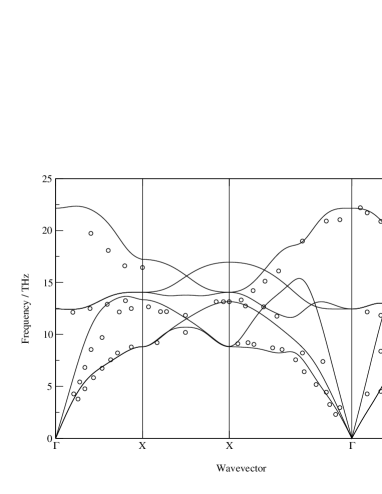
FIG. 3.: Dispersion curves for B1 MgO at lattice parameter 4.2 Å. The symmetry points in the dispersion curve are (from left to right): $\Gamma$ [000], X [001], X [011], $\Gamma$ [000] and L $[\frac{1}{2}\frac{1}{2}\frac{1}{2}]$. Note the LO–TO splitting (At $\Gamma$, LO frequency is 22.0 THz whereas TO frequency is 12.4 THz) arising from the non-analytic term of Equation 8. Also shown are Peckham’s experimental results for B1 MgO at lattice parameter 4.212 Å. Note that the reciprocal lattice vectors referred to in the results for the B1 phase are those of the cubic unit cell rather than the true reciprocal lattice vectors.

B Approximations and errors

1 Errors in ab initio total energy calculations

Total energy differences between structures calculated using density-functional theory in the generalized gradient approximation are thought to be reliable to within a few percent [22].

The cutoff energy of the plane-wave basis at 540 eV is sufficient for convergence of the total energies of the crystals to within 10 $\mu$eV per ion, several orders of magnitude less than the likely error due to the use of the GGA. The Hellmann-Feynman forces are converged to within 1 meV Å^-1, at least two orders of magnitude less than the dominant forces arising when an ion is displaced.

2 The harmonic approximation

We investigate the range of validity of the harmonic approximation. This is done for the B1 phase with lattice parameter $a=4.2$ Å.

We evaluate the force constant of the restoring force on a magnesium ion as it is displaced in the $x$-direction. The results are shown in Figure 4. It can be seen that the force constant starts to increase when the ionic displacement reaches $a_{\rm max}\approx 0.084$ Å, about 2% of the lattice parameter, at which point the potential energy is about 0.4 eV. Other displacements are similar; hence it is reasonable to assume that the forces remain linear (and the quasiharmonic assumption is valid) for temperatures up to several thousand Kelvin.

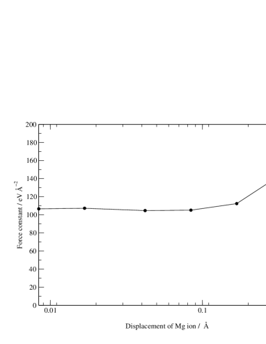
FIG. 4.: Graph of restoring force divided by the finite displacement of a Mg ion in the [100]-direction against that displacement. Results are appropriate for a $2\times 1\times 1$ supercell of B1 phase at lattice parameter 4.2 Å. The force constant is independent of the magnitude of the displacement until the displacement is at least 0.084 Å. Thereafter the restoring force increases faster than linearly with the displacement; the harmonic approximation has broken down.

3 Other sources of error

Another potential source of error is the limited size of the simulation supercells. However, the results shown in Table I for the B1 phase make it clear that interactions beyond the third-closest shell of neighbors may be safely neglected [26].

Contributions to the free energy from the thermal excitation of the valence electrons, from coupled electron-phonon excitations and from the equilibrium population of defects are thought to be negligible in comparison with the frozen-ion and lattice thermal energies [15].

Poor convergence of the Hellmann-Feynman forces can result in the violation of Newton’s third law for the matrix of force constants. Typically this results in the acoustic branches of the dispersion curve failing to pass through zero at the center of the Brillouin zone [11]. As discussed in Section II A 2, Newton’s third law is imposed on the matrix of force constants. However, even without this, the calculated acoustic branches pass very close to zero at the zone center.

The method by which long-range polarization effects are accounted for is also approximate. The effects of this are discussed below.

C Ab initio phonons

1 The B1 phase

Inelastic neutron scattering experiments were carried out by Peckham [25] and used to generate dispersion curves for the B1 phase [27]. We compare our theoretical dispersion curve with these results in Figure 3. (Note that our dispersion curve was generated for lattice parameter 4.2 Å, whereas Peckham’s results were obtained under ambient conditions where the lattice parameter is 4.212 Å.) Our theoretical results are in reasonable agreement with experiment. (The lattice parameter of $4.2$ Å corresponds to a pressure of about 7 GPa at zero temperature.)

The specific frequency density-of-states function is shown in Figure 5. Without the addition of the non-analytic term to the dynamical matrix, the longitudinal optic branch is degenerate with the transverse optic branch at the $\Gamma$-point, and this is also shown. Although only the LO branch is altered substantially, it can be seen that the inclusion of the non-analytic term has a significant effect on the density of states.

We compare sound velocities calculated from our dispersion curves with the experimental results of Reichmann et al [28] obtained using ultrasonic interferometry. Reichmann obtains a P-wave sound speed of 9119 ms^-1 in the $[100]$-direction whereas our longitudinal-acoustic mode has $\left(d\omega_{\rm LA}/dk_{[100]}\right)_{{\bf k}=0}=11367$ ms^-1.

On the other hand, in the $[111]$-direction, the experimental P-wave velocity is 10125 ms^-1 which may be compared with our theoretical value of 10818 ms^-1.

Thus Reichmann’s experimental results show a higher degree of anisotropy than do our theoretical results. The discrepancy would appear to be (at least partly) caused by the imposition of symmetry and Newton’s third law on the matrix of force constants [11]: if this procedure is not carried out then we find that $\left(d\omega_{\rm LA}/dk_{[100]}\right)_{{\bf k}=0}=10770$ ms^-1 and $\left(d\omega_{\rm LA}/dk_{[111]}\right)_{{\bf k}=0}=12651$ ms^-1. Although Reichmann’s P-wave velocities are still somewhat less than these theoretical velocities, both are now in agreement that the velocity in the $[100]$-direction is less than the velocity in the $[111]$-direction.

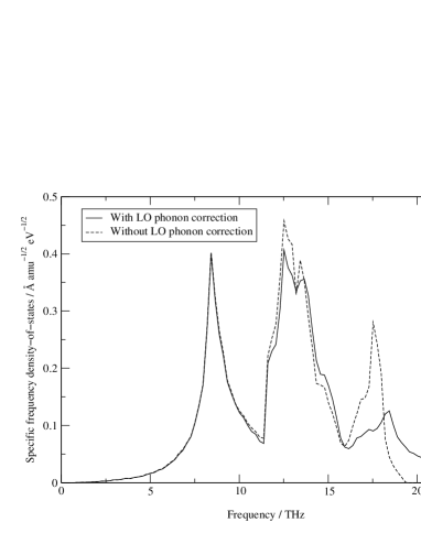
FIG. 5.: Specific frequency density-of-states for B1 phase at lattice parameter 4.2 Å with and without the inclusion of the non-analytic term in the dynamical matrix.

2 The B2 phase

Typical dispersion curves for the B2 phase at lattice parameters 2.0 Å and 2.7 Å are shown in Figures 6 and 7. At zero temperature these lattice parameters correspond to pressures of $653$ GPa and $-6$ GPa respectively.

Note the presence of unstable modes at low pressures in the dispersion curve of the B2 phase (Figure 7). We find that the B2 phase is structurally unstable for pressures below about 82 GPa. In our calculations for the phase boundary in periclase we do not require our novel method for dealing with soft modes because the imaginary frequencies are only found in the B2 phase at pressures for which the B1 phase is clearly favored.

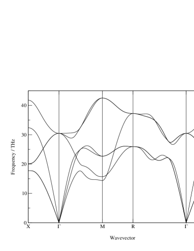
FIG. 6.: Dispersion curves for B2 MgO at a lattice parameter 2.0 Å. The symmetry points in the dispersion curve are (from left to right): X $[\frac{1}{2}00]$, $\Gamma$ [000], M $[\frac{1}{2}\frac{1}{2}0]$, R $[\frac{1}{2}\frac{1}{2}\frac{1}{2}]$, $\Gamma$ [000] and X $[\frac{1}{2}00]$.

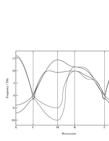
FIG. 7.: Dispersion curves for B2 MgO at a lattice constant of 2.7 Å. The symmetry points are as for Figure 6. Note the branches of imaginary phonon frequencies, indicating that the structure is mechanically unstable at this volume.

D Ab initio equation of state

We plot the pressure against specific volume for a range of temperatures in Figure 8. This is the desired thermodynamic equation of state for periclase. Also shown is a third-order Birch-Murnaghan equation of state generated from the isothermal bulk modulus and its first derivative with respect to volume, which were obtained by means of ultrasonic sound velocity measurement [29].

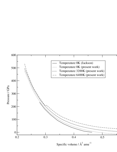
FIG. 8.: Equation of state of periclase: pressure against specific volume at various temperatures. The position of the phase transition is clearly visible as a kink in the curves. A Birch-Murnaghan equation of state generated from Jackson’s experimental results is also shown.

As a test of the validity of our results, the isothermal bulk modulus at zero temperature and external pressure (where periclase is entirely in the B1 phase) can be compared with experimental results. We calculate the bulk modulus to be $-v\left(\partial p/\partial v\right)_{T,v}=155$ GPa, whereas an experimentally determined value is $160.3\pm 0.3$ GPa [29]. The theoretical and experimental results differ by about 3%.

We may also compare the pressure derivative of the bulk modulus at zero pressure and temperature with experimental results. The bulk modulus is found to be almost, but not quite, a linear function of pressure. Fitting a straight line to the data from $-8.3$ GPa to $21.12$ GPa we find that the the gradient is $4.11$, in excellent agreement with the experimentally determined value of $4.2\pm 0.2$ [29]. It is found that the pressure derivative of the bulk modulus decreases slightly as the pressure is increased.

E Ab initio phase diagram

The theoretical phase diagram of solid periclase is shown in Figure 9. At pressures and temperatures below and to the left of the phase boundary shown in the diagram, periclase exists in the B1 phase; above and to the right of the boundary it exists in the B2 phase. Duffy [30] has shown experimentally that, at room temperature, the B1 phase is stable to pressures of at least $227$ GPa. This lies well within the B1 region of our theoretical phase diagram. It can also be noted that the B2 phase is not favored at the pressures at which it is structurally unstable.

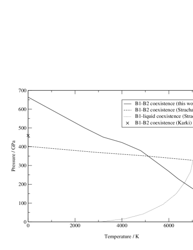
FIG. 9.: Theoretical phase diagram of periclase. The B1 phase region is below and to the left of the B1–B2 coexistence line. Also shown are other theoretical results[5, 31], including a theoretical B1–liquid phase boundary.

Also shown in Figure 9 is the theoretical phase diagram obtained by Strachan et al [31] using molecular dynamics simulation. Although qualitatively similar, the calculated position and orientation of the B1–B2 phase boundary is very different. Karki [5] obtained a B1–B2 transition pressure of 460 GPa at 0 K, which also differs substantially from that of Strachan. Figure 10 shows the Gibbs free energy plotted against pressure for the two phases at two different temperatures. The difficulty in ascertaining the transition pressures at which the curves cross is apparent. This consideration will affect all theoretical calculations of the phase diagram of periclase.

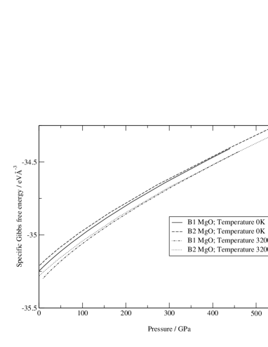
FIG. 10.: Gibbs free energy plotted against pressure for the B1 and B2 phases of periclase at two different temperatures. The transition pressure at each temperature corresponds to the point where the curves cross. The similarity of the curves for each phase means that small errors in the energies lead to large uncertainties in the transition pressures.

We confirm the difficulty in locating the transition by attempting to reproduce Karki’s zero-temperature results in which zero-point lattice vibrational energy is neglected. We simply calculate the enthalpy against pressure for the two phases using CASTEP. The results are shown in Figure 11. We find a transition pressure of  GPa, different from that of Karki (460 GPa). The possibility of a metallization transition lowering the energy of the B2 phase was investigated but found not to occur at relevant pressures.

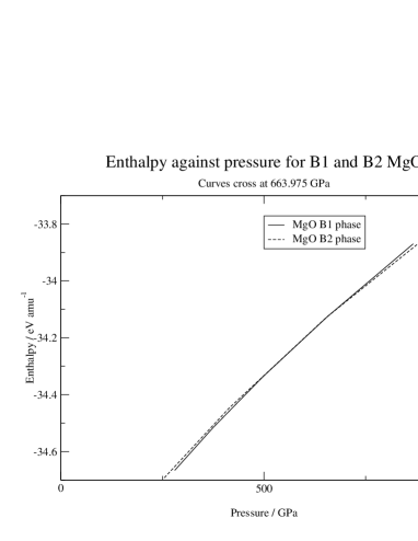
FIG. 11.: Enthalpy $h=e+pv$ plotted against pressure for the B1 and B2 phases of MgO at temperature 0 K (note that zero-point energy is not included in the results shown in this graph). The curves cross (and so the phase transition is predicted to occur) at 664 GPa. These results are obtained directly from the results of CASTEP. Note that, again, the two curves are extremely close when they cross; thus the position of the theoretical transition point is sensitive to the simulation parameters.

We consider the fractional error in unit cell volume for the B2 phase to which the difference between the specific enthalpies of the B1 and B2 phases at 451 GPa corresponds. For given unit cell enthalpy for the B2 phase, we find the fractional volume difference as:

$$\left|\frac{\Delta V}{V}\right|=2\left|\frac{h_{B2}-h_{B1}}{h_{B2}+h_{B1}}\right|,$$ (41)

where $h_{B1}=-34.4043$ eVÅ^-3 and $h_{B2}=-34.3978$ eVÅ^-3 are the specific enthalpies of the two phases at 451 GPa. Thus a discrepancy of $\Delta V/V\times 10^{-4}\approx 0.02$% in the volume of either phase would correspond to a 200GPa change in the transition pressure. This illustrates the sensitivity of the transition point to the details of how the total energy calculations are carried out.

We use the generalized gradient approximation and ultrasoft pseudopotentials[20, 21], whereas Karki used the local density approximation and $Q_{c}$ tuned pseudopotentials [32, 33]. The difference between calculated volume using these two methods is typically of the order of 5%; hence this is likely to be responsible for the difference between our results and Karki’s.

The Clausius-Clapeyron equation for the coexistence line between two phases in $(p,T)$-space is:

$$\frac{dp}{dT}=\frac{\Delta s}{\Delta v},$$ (42)

where $p(T)$ is the coexistence line and $\Delta s$ and $\Delta v$ are the specific entropy and volume differences between the two phases across the line. At zero temperature the entropy of the two phases should be zero by the third law of thermodynamics which is valid within our method (though not, e.g. in classical MD[31]); therefore, provided the phases have different densities, the coexistence line should satisfy $dp/dT=0$ at $T=0$. Figure 9.) does not appear to satisfy this requirement.

The explanation for this apparent discrepancy lies with the fact that the densities of the two phases are very similar (and converging) at their predicted zero-temperature transition point: the specific volumes of the B1 and B2 phases are 0.202 ųamu^-1 and 0.198 ųamu^-1 respectively.

V Conclusions

We have described an extension to the quasiharmonic method that allows the free energy contribution from “soft” phonons in dynamically stabilized crystals to be evaluated. Our approach is based on a form of potential double-well different to that used in previous work on soft phonons: a parabola-plus-Gaussian form that has the advantage of being harmonic in both the low- and high-temperature limits.

We argue that the first-order nature of the phase transitions found using our extended quasiharmonic method arises because of the coupling of the relevant phonon to strain in the crystal. Without this coupling, the transition would be second-order. We have suggested a criterion for judging when a second-order soft-mode phase transition has occurred, taking into account the quantum mechanical nature of the problem.

At energies less than the height of the central barrier in our symmetric potential double-well, the allowed energy levels consist of near-degenerate pairs. Hence we suggest there must exist extremely low-frequency photon absorption peaks for soft-mode materials in their low-temperature phase, corresponding to photon-induced transitions between such pairs.

We have evaluated the equation of state and the phase boundary for the B1–B2 transition in periclase using ab initio calculations in the quasiharmonic approximation. We predict that this transition will occur, but that it is well outside the ranges encountered inside the Earth. Locating the B1–B2 phase boundary with precision is difficult, however, because the Gibbs free energy curves of the two phases are very similar when they cross.

VI Acknowledgments

We would like to thank D. C. Swift and M. C. Warren for helpful discussion. This work was carried out as part of the UKCP-MSI collaboration, supported by EPRSC GR/N02337. Copies of the codes used for the free energy calculations are available from the authors on request.

Position of Mg atom	Magnitude of [001]-component
	of force / eVÅ-1
(0,0,0)	0.13424
(0.5,0.5,0.0625)	0.03356
(0,0,0.125)	0.00981
(0.5,0.5,0.1875)	0.00006

TABLE I.: Magnitude of the component of force in the [001]-direction when the Mg ion at (0,0,0) is displaced in the [001]-direction by 0.05% of the length of a $1/\sqrt{2}\times 1/\sqrt{2}\times 8$ supercell. Coordinates are given as fractions of the supercell dimensions. (These results are for B1 MgO at lattice parameter 4.2 Å.)

REFERENCES

- [1] D. C. Wallace, Thermodynamics of crystals, John Wiley and Sons, New York (1972).
- [2] M. Born and K. Huang, Dynamical theory of crystal lattices, Oxford Univ. Press, London and New York (1956).
- [3] W. Zhong, D. Vanderbilt and K. M. Rabe, Phys. Rev. B 52, 6301 (1995).
- [4] M. C. Warren, G. J. Ackland, B. B. Karki and S. J. Clark, Mineralogical Magazine 62, 585 (1998).
- [5] B. B. Karki, G. J. Ackland and J. Crain, J. Phys.: Condens. Matter 9, 8579 (1997).
- [6] M. C. Warren and G. J. Ackland, Phys. Chem. Min. 23 (1996).
- [7] M. C. Warren, PhD thesis, The University of Edinburgh (1997).
- [8] G. Fiquet, A. Dewaele, D. Andrault, M. Kunz and T. Le Bihan, Geophys. Res. Lett. 27 , 21 (2000).
- [9] K. Parlinski and Y. Kawazoe, Eur. Phys. J. B 16, 49 (2000).
- [10] A. R. Oganov, J. P. Brodholt and G. D. Price, Phys. Earth Planet Interiors 122, 277 (2000).
- [11] G. J. Ackland, M. C. Warren and S. J. Clark, J. Phys.: Condens. Matter 9, 7861 (1997).
- [12] K. Parlinski, J. Łażewski and Y. Kawazoe, J. Phys. Chem. Solids 61, 87 (2000).
- [13] N. W. Ashcroft and N. D. Mermin, Solid state physics, Saunders College Publishing (1976).
- [14] W. Cochran and R. A. Cowley, J. Phys. Chem. Solids 23, 447 (1962).
- [15] D. C. Swift and G. J. Ackland, Phys. Rev. B in press (2001); D. C. Swift, PhD thesis, The University of Edinburgh (2000).
- [16] A. D. Bruce, Adv. Phys. 29, 117 (1980).
- [17] L. Stixrude, and R. E. Cohen, Nature 364, 613 (1993).
- [18] P. E. Blöchl, O. Jepsen and O. K. Andersen, Phys. Rev. B 49, 16223 (1994).
- [19] CASTEP 3.9 academic version, licensed under the UKCP-MSI Agreement www.cse.clrc.ac.uk/Activity/UKCP (1999).
- [20] J. P. Perdew, J. A. Chevary, S. H. Vosko, K. A. Jackson, M. R. Pederson, D. J. Singh and C. Fiolhais, Phys. Rev. B 46, 6671 (1992).
- [21] D. Vanderbilt, Phys. Rev. B 41, 7892 (1990).
- [22] M. C. Payne, M. P. Teter, D. C. Allan, T. A. Arias and J. D. Joannopoulos, Rev. Mod. Phys. 64, 1045 (1992).
- [23] H. J. Monkhorst and J. D. Pack, Phys. Rev. B 16, 2981 (1977).
- [24] K. Kunc, R. J. Needs, O. J. Nielsen and R. M. Martin, Symmetry and Special Points Program K290 (unpublished).
- [25] G. Peckham, Proc. Phys. Soc. 90, 654 (1967).
- [26] Apart from the non-analytic dipole term, which is calculated separately.
- [27] M. J. L. Sangster, G. Peckham and D. H. Saunderson, J. Phys. C 3, 1026 (1970).
- [28] H. J. Reichmann, S. D. Jacobsen, S. J. Mackwell and C. A. McCammon, Geophys. Res. Lett. 27, 799 (2000).
- [29] I. Jackson and H. Niesler, in High Pressure Research in Geophysics, 93 (1982).
- [30] T. S. Duffy, R. J. Hemley and H.-K. Mao, Phys. Rev. Lett. 74, 1371 (1995).
- [31] A. Strachan, T. Çağin and W. A. Goddard, Phys. Rev. B 60, 15 084 (1999).
- [32] J.P Perdew and A Zunger Phys. Rev. B 23 5048 (1981).
- [33] J.S. Lin, A. Qteish, M.C. Payne and V. Heine Phys. Rev. B 47 4174 (1993); M.H. Lee Advanced pseudopotentials for large scale electronic structure calculations, PhD Thesis, University of Cambridge, UK, (1995).