Random Geometric Graphs

Abstract

We analyse graphs in which each vertex is assigned random coordinates in a geometric space of arbitrary dimensionality and only edges between adjacent points are present. The critical connectivity is found numerically by examining the size of the largest cluster. We derive an analytical expression for the cluster coefficient which shows that the graphs are distinctly different from standard random graphs, even for infinite dimensionality. Insights relevant for graph bi-partitioning are included. PACS: 05.10.Ln, 64.60.Ak, 89.75.Da
KEY WORDS: Networks, percolation, phase transitions, random graphs, scaling, graph bi-partitioning.

1 Introduction

The interest in complex networks has exploded over the last five years [1, 2] where data on very large networks like the WWW [3, 4, 5], collaborations in the scientific community [6], transportation [7], movie actor collaborations [8] etc. have become accessible.

Random graphs are often used to model complex networks [9]. Ever since Erdös and Rényi’s groundbraking work more than forty years ago [10], intense theoretical research on random graphs has been taking place  [4, 11, 12, 13]. In contrast to random graphs the interactions between the sites in a lattice are usually between nearest neighbours, reflecting a myopic world. Lattices are therefore often said to be at the other end of the spectrum of network models [14, 15].

Properties of real networks like robustness [16, 17], growth [11, 18, 19, 20], and topology have attracted much attention, primarily from physicists. It has been consistently shown that many of the networks possess small world characteristics [8, 21, 22]. Like random graphs, small world networks are characterized by short average distances between any two sites, and by a high degree of localness, much like in lattices. However, individually, random graphs and lattice models in their pure forms are poor models of many real world networks. One could argue that high-dimensional lattices have the necessary high clustering and low average path length, though this has not been explored much [23]. In the current paper we provide results on high-dimensional systems.

A random geometric graph (RGG) is a random graph with a metric. It is constructed by assigning each vertex random coordinates in a $d$-dimensional box of volume 1, i.e. each coordinate is drawn from a uniform distribution on the unit interval. RGGs have been used sporadically in real networks modeling [24] and extensively in continuum percolation [25, 26, 27, 28, 29], but almost exclusively in two and three dimensions. Although RGGs are the continuum version of lattices, they deserve some attention of their own, since percolating continuum systems display behaviour that lattices are incapable of [30]. In addition, the connectivity in RGGs can be increased in a more natural way than by adding new bonds randomly in lattices.

Recently, continuum percolation has been used in the study of the stretched exponential decay of the correlation function in random walks on fractals and the conjectured relation to relaxation in complex systems [31]. However, continuous systems in general and RGGs in particular are relevant whenever we need a multi-dimensional system with a metric, as for example when modeling the spread of diseases [32].

In this paper we study RGGs in arbitrary dimensions. In low dimensions the systems are dominated by local interactions. For higher dimensions RGGs are usually believed to approach standard random graphs, which we show is true only in some respects. We focus on ‘phase transitions’ [13, 33, 34] at the percolation threshold by looking at the size of the largest cluster, and we determine how the value of the critical parameter in RGGs approaches that of random graphs as the dimension increases. We also extract the distribution of cluster sizes in the critical region. Furthermore, an expression for the cluster coefficient, a quantity that has attracted much interest in network theory recently, is derived. Results relevant for graph bi-partitioning are established. Finally, we discuss how to implement random geometric graphs efficiently.

The layout of this paper is as follows. In Section 2 and 3 we describe random graphs and random geometric graphs, respectively. In Section 4 we present our results, and Section 5 contains the details regarding the implementation. Finally, in Section 6 we sum up.

2 Random Graphs

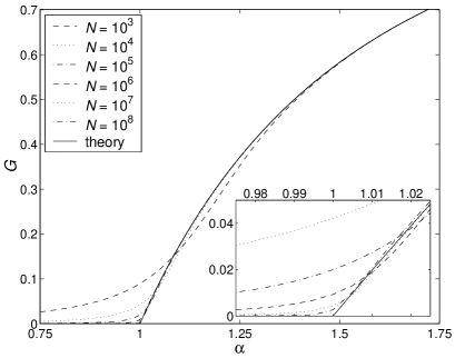
Figure 1: The size of the largest cluster in random graphs as a function of the connectivity. Note that for $N>10^{6}$ the Monte Carlo data is almost indistinguishable from the theoretical result in Eq. (3). Error bars are not shown since they are in all cases less than the width of the lines. Inset: A closer look at the percolation threshold $\alpha_{c}=1$.

Random graphs consist of $N$ vertices (points/sites) and $K$ edges (lines) where each possible edge is present with probability $p$, i.e. $K=pN(N-1)/2$. To keep the discussion independent of the system size $N$, graphs are often characterized by the connectivity (degree) $\alpha=2K/N=pN$, i.e. the average number of connections per vertex, instead of $K$ or $p$. As the connectivity increases clusters of vertices appear, where a cluster consists of all vertices linked together by edges, directly or indirectly.

The size of the largest cluster in the macroscopic limit $N\rightarrow\infty$ can be calculated analytically [10, 12]. It is $NG(\alpha)$, where

$$G(\alpha)=1-\frac{1}{\alpha}\sum_{n=1}^{\infty}\frac{n^{n-1}}{n!}(\alpha e^{-\alpha})^{n}.$$ (1)

By the use of [12]

$$y=\sum_{n=1}^{\infty}\frac{n^{n-1}}{n!}x^{n}\ \ \Leftrightarrow\ \ x=ye^{y}$$ (2)

we can invert Eq. (1), getting

$$\alpha(G)=-\frac{1}{G}\log(1-G).$$ (3)

from which it is trivial to show that $\alpha_{c}=1$. With Eq. (3) it is an easy task to plot the fraction of vertices in the largest cluster—the giant component—as done in Fig. 1, where we see the prototype of a phase transition in combinatorial problems.

In random graphs the probability distribution of edges $p_{k}$ is binomial

$$p_{k}=\left(\!\!\begin{array}[]{c}N\\ k\end{array}\!\!\right)p^{k}(1-p)^{N-k}\simeq\frac{\alpha^{k}e^{-\alpha}}{k!},$$ (4)

where the approximation resulting in the Poisson distribution is valid for large systems sizes $N$, which is exactly the limit in which we are interested. The critical connectivity $\alpha_{c}$ for graphs with arbitrary random degree distribution $p_{k}$ has recently been derived by other techniques than those originally leading to Eq. (1) [4, 36, 37]. Unfortunately, we cannot use these results in connection with random geometric graphs, as will become clear in the next section.

3 Random Geometric Graphs

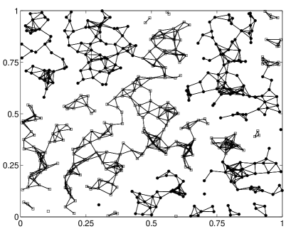
Figure 2: A $2D$ random geometric graph with $N=500$ and $\alpha=5$. The graph is bi-partitioned—see Section 4. There are no edges across the boundaries, i.e. the boundary conditions are open, not continuous.

A $d$-dimensional random geometric graph (RGG) is a graph where each of the $N$ vertices is assigned random coordinates in the box $[0,1]^{d}$, and only points ‘close’ to each other are connected by an edge. The degree distribution of a RGG with average connectivity $\alpha$ is therefore given by Eq. (4) as well. However, a RGG is a special kind of random graph with properties not captured by the theoretical tools mentioned above. For one thing, the probability that three vertices are cyclically connected is different in random graphs and RGGs, regardless of the degree distribution of the random graph.

RGGs are sometimes named spatial graphs [8]. Fig. 2 illustrates a RGG in $2D$. As in lattices, different boundary conditions can be applied. We will see that toroidal (continuous) boundary conditions make a vital difference compared to having open boundary conditions.

The volume of a $d$-dimensional (hyper)sphere with radius $r$ is

$$V_{sphere}=\frac{{\pi}^{d/2}r^{d}}{\Gamma(\frac{d+2}{2})},$$ (5)

where $\Gamma(x)$ is the gamma function. This volume is needed in order to find the edges in RGGs.

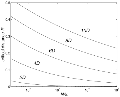
Figure 3: The critical distance in random geometric graphs in various dimensions. Points within this distance of each other are connected by an edge. The critical distance is equivalent to the radius $R$ of the excluded volume associated with each point.

To ‘visualise’ a RGG in general, one can think of a box filled with small spheres with radius $r$ and volume $V$ given by Eq. (5), where points are connected by an edge only if the distance between their centers is $<2r$, i.e. if the spheres overlap. Since the total volume of our box is 1, the probability that two arbitrarily chosen vertices are connected is equal to the volume of a sphere with radius $R=2r$. In continuum percolation theory this volume is denoted the excluded volume $V_{ex}$, where $V_{ex}=2^{d}V$ in a RGG. The excluded volume is the basic quantity of interest because it is directly related to the connectivity

$$\alpha=Np=NV_{ex},$$ (6)

from which it is clear why the connectivity is frequently called the total excluded volume of the system. Eqs. (5) and (6) give us

$$R=\frac{1}{\sqrt{\pi}}\left[\frac{\alpha}{N}\Gamma\left(\frac{d+2}{2}\right)\right]^{\frac{1}{d}}.$$ (7)

Fig. 3 shows the radius $R$ of the excluded volume as a function of $N/\alpha=1/p=1/V_{ex}$. $R$ decreases monotonically: for a given connectivity $\alpha$ the spheres have to become smaller when more vertices are added to the graph.

Eq. (7) provides us with the required relation between $\alpha$ and $R$ when creating a RGG. The distance between every pair of vertices must be calculated, and an edge is added if the distance is less than $R$. Thus, it seems unavoidable to have a runtime of $O(N^{2})$ making it unfeasible to investigate as large systems as with random graphs—see Fig. 1—where the number of calculations for a given $\alpha$ needed to create all the edges is $O(N)$. To overcome this obstacle we have designed a data structure which is described in Section 5, with a runtime of $O(N^{\beta})$ where $\beta\simeq 1.3$. This allows us to study RGGs with up to $N=4^{11}>4\cdot 10^{6}$ vertices, which is more than an order of magnitude larger than usually accomplished [38].

4 Results

In our simulations of RGGs we define $\alpha_{c}$ to be the lowest connectivity at which the fraction of vertices in the largest cluster is $>0$ in the macroscopic limit. We make the bold claim that the systems we are able to analyse consist of enough points to make the critical connectivity almost as sharply defined as in Fig. 1. However, our main purpose is not to derive high precision percolation thresholds. Instead, we are more interested in the critical connectivity as a function of the dimension of the RGGs.

In this paper we express our threshold values in terms of $\alpha$. Other popular choices are the fractional volume $s$ occupied by the spheres [30] or the density $N$ of spheres. The relation between these parameters at the percolation threshold is

$$\alpha_{c}=N_{c}V_{ex}=-2^{d}\ln(1-s_{c})$$ (8)

(see e.g. [25] for a derivation). Usually, in continuum percolation the volume $V$ of each sphere is fixed while $N$ is the independent variable in a system of size $[0,L]^{d}$. The approach of measuring $N_{c}$ or $s_{c}$ for various values of $L$ has been used in both two [39] and three [38] dimensions, i.e. for discs and spheres, where the critical values are determined by the use of finite size scaling. This procedure resembles site percolation in lattices. From the previous sections it is clear that we take a route closer to bond percolation in lattices by fixing $L=1$ while tuning $\alpha$ for different values of $N$. In Section 5 we describe how this has been carried out in practice.

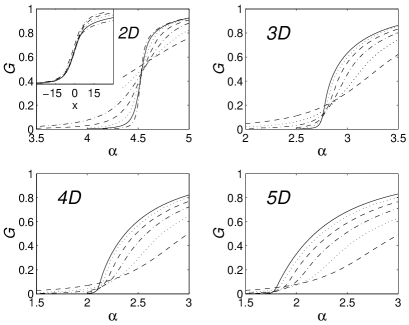
Figure 4: The average fraction of vertices in the largest cluster for various system sizes $N$ (see the legend in Fig. 5) in random geometric graphs with no edges across the boundaries. The inset in $2D$ illustrates a finite size scaling—see the text. In higher dimensions the general shape of the curves as $N$ increases is nontrivial. Compare with Fig. 5. Error bars are $<10^{-3}$ for all curves and therefore omitted.

The Size of the Largest Cluster

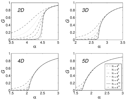
Figure 5: Like Fig. 4 but with continuous boundary conditions. We see that the point at which the largest cluster becomes macroscopic is sharply defined and can immediately be determined by the eye with high precision (Table 1). The overall behaviour of the graphs for higher dimensions is much closer to Fig. 1 than Fig. 4 is. As $d$ increases the $\alpha$-interval where there is a significant difference between curves with different $N$ get smaller and smaller. Error bars are $<10^{-3}$ for all curves and therefore omitted.

Let $G_{d}(\alpha)$ denote the fraction of vertices in the largest cluster in $d$ dimensions. Since a RGG in the limit of infinite dimension is often assumed equivalent to a random graph, we expect that Eq. (3) provides us with an expression for $G_{\infty}(\alpha)$. But what does $G_{d}(\alpha)$ look like for finite $d$? And what is the behaviour of $\alpha_{c}(d)$? How does it approach $\alpha_{c}(\infty)$ as $d$ increases? These are the questions addressed in this and the following section.

Figs. 4 and 5 illustrate the average size of the largest cluster in RGGs in 2, 3, 4, and 5 dimensions with and without toroidal boundary conditions. The curves correspond to $N=4^{k}$ vertices with $k=5,6,...,11$, where the larger systems display the sharpest transitions. The legend in Fig. 5 applies to all diagrams in Figs. 4 and 5. In these 8 diagrams each curve is based on 300 data points. In other words, $G_{d}(\alpha)$ is calculated in intervals of $\Delta\alpha=0.005$ resulting in the smooth lines in the figures. For every data set we have averaged over enough runs for error bars to be completely negligible.

Since continuous boundary conditions mean addition of extra edges, the size of the largest component $G(\alpha)$ obviously grows faster in Fig. 5 than in Fig. 4, especially in the smaller systems. These relatively few extra edges make a decisive difference, connecting vertices not already in the same cluster. Since toroidal systems are models of bulk systems, $G$ is much less $N$-dependent in that case. However ‘unphysical’ RGGs with open boundaries may seem, they are the most popular RGG version in the literature. Consequently, we consider them alongside the continuous case.

From Figs. 4 and 5 we see that the continuous boundary conditions make the transition where $G>0$ more abrupt, but that an estimation of $\alpha_{c}$ does not depend much on the boundary conditions if only we base our judgment on large enough systems. This is confirmed in the inset of Fig. 4, where $\alpha_{c}=4.53$ is obtained by finite size scaling, i.e. plotting $G(x)$ where $x=N^{1/\nu}(\alpha-\alpha_{c})$. However, it is clearly easier to make precise estimates of the critical connectivity with than without continuous boundary conditions. We note in passing that the exponent $\nu=3$ is equal to the value of $\nu$ found in random graphs [13].

The Critical Connectivity

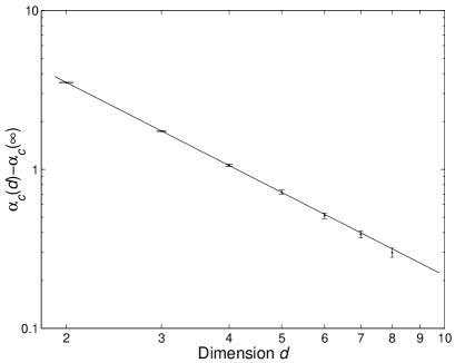
Figure 6: Scaling of the critical connectivity as a function of the dimension of the random geometric graphs reveals a power-law relation, Eq. (9). For $d\leq 5$ the data points are estimated by close inspection of Fig. 5. For $d>5$, $\alpha_{c}$ is based on runs with $N=4^{10}$ points. Error bars are included. See Table 1.

With numerically obtained knowledge of $G(\alpha)$, it is possible to extract $\alpha_{c}$. The procedure is simple. By inspection of Fig. 5 we can estimate $\alpha_{c}$ for $d\leq 5$. To obtain further data points we have run our algorithm on RGGs with $N=4^{10}$ for systems of larger dimensions as well. Though this results in increased runtime per graph, the results get more homogeneous and fewer runs are needed in order to get a decent estimate of $G_{d}(\alpha)$. Our findings presented in Table 1 and Fig. 6 strongly suggest that

$$\alpha_{c}(d)=\alpha_{c}(\infty)+Ad^{-\gamma},$$ (9)

where $\alpha_{c}(\infty)=1$, $\gamma=1.74(2)$ and $A=11.78(5)$. As expected, Eq. (9) predicts that $\alpha_{c}(\infty)$ is equal to $\alpha_{c}$ in random graphs, confirming that RGGs and random graphs become more and more similar as $d$ increases. However, when we derive the cluster coefficient, we will see that this is not true in all respects.

Finally, we note that our findings are in accordance with the most precise estimates that we know of: $\alpha_{c}=4.51223(5)$ [29] and $\alpha_{c}=2.734(6)$ [38] in $2D$ and $3D$, respectively, obtained by the use of finite size scaling. For $d>3$ we have not been able to find any estimates of $\alpha_{c}$ to compare with [40].

The Distribution of Cluster Sizes

$d$	2	3	4	5	6	7	8
$\alpha_{c}$	4.52	2.74	2.06	1.72	1.51	1.39	1.30
$\pm$	0.01	0.01	0.02	0.02	0.02	0.02	0.02

Table 1: The critical connectivity $\alpha_{c}$ in random geometric graphs of dimension $d$ with continuous boundary conditions. The data are plotted in Fig. 6. The estimated errors in $\alpha_{c}$ in the last row are rather conservative.

Having examined the size of the largest cluster and the critical connectivity, we now look at the distribution of cluster sizes in RGGs.

Figure 7: The distribution of cluster sizes in $3D$ random geometric graphs with $N=1000$ vertices in the vicinity of the critical connectivity $\alpha_{c}=2.74$. The inset shows that for $\alpha\simeq\alpha_{c}$ the cluster sizes are given by a power-law. For each value of $\alpha$ the data points are based on $10^{6}$ graphs.

The inset illustrates the scale free power-law distribution at $\alpha=2.6$. Right below $\alpha_{c}$, clusters of all sizes can be encountered. The small hump at large cluster sizes is always present because the clusters cannot contain more than all of the vertices. The clusters pile up when their size approaches this boundary, in this case a cluster size of $1000$, just below the inevitable cut-off.

Our simulations show that for $\alpha$ significantly below $\alpha_{c}$ the distribution is approximately exponential. As the connectivity increases the distribution becomes power-law-like. As $\alpha$ is further increased the distribution is separated in two parts; there are no clusters of medium size, only the largest macroscopic cluster and a few small ones around it. We have observed this overall behaviour in all our tests of the distribution of cluster sizes in various dimensions.

Fig. 7 shows our data in $3D$. For $\alpha=2.1$ ($\cdot$) the data points lie on an almost straight line indicating an exponential distribution. Increasing the connectivity to $\alpha=2.4$ ($\triangle$) results in a broader distribution that is no longer exponential. Right at the critical connectivity ($\circ$) the distribution flattens out. Clusters of all sizes are observed. Right above $\alpha_{c}$ ($\diamond$) two separate regions begin to materialise. Already at $\alpha=3.3$ ($\star$) the largest cluster makes it highly unlikely that a cluster of medium size can be present as well. The distribution is cut in two.

The Cluster Coefficient

In network theory the cluster coefficient $C$ is an often calculated quantity [1, 21, 23], which is defined in the following way. Let the vertices $i$ and $j$ be connected directly to a common vertex $k$. $C$ is then the probability that vertex $i$ and vertex $j$ are directly connected as well. From this we see that the cluster coefficient is a measure of the ‘cliquishness’ of the graph. In this section we derive $C=C_{d}$ analytically in arbitrary dimensions $d$, showing that $C_{d}$ decreases in an exponential fashion.

To determine $C_{d}$ we make use of the concept of the excluded volume $V_{ex}$. If we again use the vertices $i$, $j$, and $k$, then $i$ and $j$ must both be within the excluded volume of $k$. Put differently, the probability that $i$ and $j$ are connected is equal to the probability that two randomly chosen points in a sphere of volume $V_{ex}$ and radius $R$ is less than a distance $R$ apart. In other words, given the coordinates of vertex $i$ the probability that there is an edge between $i$ and $j$ is equal to the fraction of the excluded volume of vertex $i$ that lies inside the excluded volume of $k$. By averaging over all points in $V_{ex}$ we get the cluster coefficient $C_{d}$.

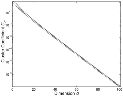
Figure 8: The cluster coefficient $C$ in random geometric graphs. The full line is the asymptotic solution, Eq. (13), valid for large $d$ only.

The task of calculating $C_{d}$ is considerably simplified by the spherical symmetry of the problem. The fractional volume ‘overlap’ $\rho_{d}$ of two spheres only depends on the distance $r$ between the centers and not on any angular parts, i.e. $\rho_{d}=\rho_{d}(r)$. In general, the cluster coefficient can therefore be written as

$$C_{d}=\frac{1}{V_{ex}}\int_{V_{ex}}\rho_{d}(r)\textrm{d}V.$$ (10)

In Appendix A we derive that

$$C_{d}=\left\{\begin{array}[]{ll}1-H_{d}(1)&\mbox{even $d$}\\ \\ \frac{3}{2}-H_{d}(\frac{1}{2})&\mbox{odd $d$}\end{array}\right.$$ (11)

where

$$H_{d}(x)=\frac{1}{\sqrt{\pi}}\sum_{i=x}^{d/2}\frac{\Gamma(i)}{\Gamma(i+\frac{1}{2})}\left(\frac{3}{4}\right)^{i+\frac{1}{2}}.$$ (12)

When $d$ is large Eq. (11) reduces to (see Appendix A)

$$C_{d}\sim 3\sqrt{\frac{2}{\pi d}}\left(\frac{3}{4}\right)^{\frac{d+1}{2}}.$$ (13)

The cluster coefficient is plotted in Fig. 8 ($\circ$) together with the asymptotic solution in Eq. (13) (full line).

Eq. (11) shows that the cluster coefficient is a purely geometric quantity depending only on the dimension $d$; neither the connectivity $\alpha$ nor the system size $N$ are present. In random graphs $C=\alpha/N$, since there is per definition no correlation between edges. So, in contrast to what is usually believed, RGGs are not identical to random graphs when $d\rightarrow\infty$.

In higher dimensions, the cluster coefficient in RGGs becomes exceedingly small. This peculiar fact can be explained by noting that the distribution of distances between two connected vertices gets more and more peaked at the maximal distance $R$ as $d$ increases. This implies that if the vertices $i$ and $j$ are both connected to vertex $k$ in a high-dimensional space, then it is highly unlikely that $i$ and $j$ are directly connected by an edge as well. Only in low dimensions are RGGs dominated by small loops. On the contrary, the way that a standard random graph is designed implies a cluster coefficient which can only be interpreted statistically, and not geometrically. Despite the fact that $\alpha_{c}=1$ in both random graphs and RGGs of infinite dimensionality, they do not have the same topology.

Graph Bi-partitioning

Random geometric graphs are useful outside network modeling and percolation theory as well. In this section we look at RGGs in relation to graph bi-partitioning, a well known problem in combinatorial optimization.

The NP-hard problem of partitioning a graph with $N$ vertices in two subsets with $N/2$ vertices each, in such a way that the cutsize $E$, i.e. the number of edges between vertices in different subsets, is minimized, is called the graph bi-partitioning (GBP) problem. Fig. 2 illustrates a bi-partitioned RGG, where $N/2$ of the points are marked by squares, the other half being dots.

The GBP problem of RGGs with open boundary conditions has been tested by various heuristics [41, 42, 43]. In this section we use our numerical findings to establish the critical connectivity in relation to GBP. Additionally, for $\alpha>\alpha_{c}^{\scriptscriptstyle{GBP}}$ we argue that the cutsize $E$ depends on $N$ and $\alpha$ in a simple way.

In GBP the connectivity is critical when $G=1/2$. As soon as the largest cluster contains more than half of the vertices, it becomes impossible to bipartition the graph without violating any edges. For random graphs Eq. (3) immediately gives us $\alpha_{c}^{\scriptscriptstyle{GBP}}=2\ln 2\simeq 1.386$.

$d$	2	3	4	5
$\alpha_{c}^{\scriptscriptstyle{GBP}}$	4.52	2.84	2.275	1.99
$\pm$	0.02	0.01	0.005	0.005

Table 2: The critical connectivity $\alpha_{c}^{\scriptscriptstyle{GBP}}$ in random geometric graphs with toroidal boundary conditions. Only in $2D$ does $\alpha_{c}^{\scriptscriptstyle{GBP}}$ depend noticably on $N$ for $N>1000$ (see Fig. 5). Note that without continuous boundaries Fig. 4 shows that $\alpha_{c}^{\scriptscriptstyle{GBP}}$ is highly size-dependent for $d>2$. The estimated errors in $\alpha_{c}^{\scriptscriptstyle{GBP}}$ in the last row are on the safe side.

In RGGs $\alpha_{c}^{\scriptscriptstyle{GBP}}(d)$ can be extracted in the same way as $\alpha_{c}$ was in Section 4. Our numerical findings in RGGs with continuous boundary conditions are presented in Table 2. We stress that the results are valid only for large $N$, as a closer look at Fig. 5 reveals. In $2D$ the average fraction of vertices in the largest cluster is independent of $N$ only for $\alpha>\alpha_{c}^{\scriptscriptstyle{GBP}}$. This means that if one looks at GBP in $2D$ with $N=1000$, one cannot use the value of $\alpha_{c}^{\scriptscriptstyle{GBP}}$ in Table 2. In higher dimensions the interval around $\alpha_{c}$ where $G_{d}(\alpha)$ is size-dependent gets smaller and does not play a role in relation to GBP.

With open boundary conditions the picture is messy, as Fig. 4 shows. In this case $G(\alpha)$ is highly $N$-dependent, and it is not possible to speak of a critical connectivity $\alpha_{c}^{\scriptscriptstyle{GBP}}$ without specifying $N$. This is true despite the fact that $G(\alpha)$ is an averaged quantity, i.e. for small $N$ will a fraction of the graphs contain a cluster with more than $N/2$ vertices even when $\alpha<\alpha_{c}^{\scriptscriptstyle{GBP}}$. Fig. 4 clearly shows that $\alpha_{c}^{\scriptscriptstyle{GBP}}$ is a decreasing function of $N$ for $d>2$. In $2D$ however, all curves cross at almost the same (pivotal) point, and it is reasonable to speak of $\alpha_{c}^{\scriptscriptstyle{GBP}}$ without specifying $N$. As the inset in Fig. 4 shows this would lead to an estimate of $\alpha_{c}^{\scriptscriptstyle{GBP}}=4.53(1)$, close to $\alpha_{c}^{\scriptscriptstyle{GBP}}$ in RGGs with toroidal boundary conditions.

The size of the largest cluster near $\alpha_{c}$ grows so rapidly in $2D$ that $\alpha_{c}=\alpha_{c}^{\scriptscriptstyle{GBP}}$ cannot be ruled out on the basis of our numerical data. This is true with both open and continuous boundary conditions. However, as this would imply that the phase transition is of 1st order in $2D$ only, we believe that the two critical connectivities are close but not identical.

When bi-partitioning a RGG, it is obvious that the ‘area of contact’ [44] between the two subsets in the optimal configuration must be close to a minimum. In $2D$ this means that the best achievable partition must be close to simply cutting the graph in two at the coordinate values $x_{1}=1/2$ or $x_{2}=1/2$. This observation is especially relevant for large connectivities where the cutsize is, fluctuations neglected, proportional to the length of the dividing line. All this tentatively indicates how the cutsize $E$ in GBP behaves as a function of $N$ and $\alpha$ by looking at RGGs partitioned at $x_{i}=1/2$, where $1\leq i\leq d$. As we are about to argue, we expect a scaling relation like [45, 46]

$$E_{d}\propto N^{1/\nu}\alpha^{\beta}(d),$$ (14)

where the exponents $\nu$ and $\beta$ only depend on the dimension of the RGG.

The exponents in Eq. (14) can be determined in the following way. Given the radius $R$ of the excluded volume of each vertex, the cutsize must be proportional to $NR$, since only vertices with $1/2-R<x_{i}<1/2$ contribute to the cutsize (to avoid counting the violated edges twice we only look at the vertices at one side of the partitioning plane at $x_{i}=1/2$), times the average number of violated edges per vertex in this region, which is proportional to $NR^{d}$. In other words,

$$E_{d}\propto N^{2}R^{d+1}.$$ (15)

If instead of $R$ we want to express the result in terms of $\alpha(d)\propto NR^{d}$, we get

$$1/\nu=1-\frac{1}{d},\;\;\;\beta=1+\frac{1}{d}.$$ (16)

Since $E\propto N^{2}$ in Eq. (15), the relation $1/\nu+\beta=2$ holds in arbitrary dimensions.

Now, it is obvious that the scaling Ansatz is reasonable only for $\alpha>\alpha_{c}^{\scriptscriptstyle{GBP}}$. As Fig. 2 illustrates, the optimal partition at $\alpha\sim\alpha_{c}^{\scriptscriptstyle{GBP}}$ is highly complex and not at all close to a straight line. If we incorporate that $E=0$ for $\alpha<\alpha_{c}^{\scriptscriptstyle{GBP}}$ and replace Eq. (14) with

$$E_{d}\propto N^{1/\nu}(\alpha(d)-\alpha_{c}^{\scriptscriptstyle{GBP}})^{\beta},$$ (17)

we do not expect Eq. (16) to hold if we focus only on a region near the critical connectivity. By the use of extremal optimization, a heuristic that works particularly well near phase transitions in hard combinatorial problems, Boettcher and Percus [45, 46] have found $\alpha_{c}^{\scriptscriptstyle{GBP}}\simeq 4.1$, $1/\nu\simeq 0.6$ and $\beta\simeq 1.4$ in $2D$ for $4<\alpha<6$, not far off our estimates in Eq. (16) valid for large connectivities. Note that the low estimate of $\alpha_{c}^{\scriptscriptstyle{GBP}}$ is expected; the algorithm does not always find the best partition, and some graphs with $\alpha<\alpha_{c}$ does have $E>0$.

5 Implementation

The implementation is of major importance when studying random geometric graphs, since a straightforward check of all possible edges between the $N$ points will result in unfeasible runtimes $O(N^{2})$. We now outline how our program works and describe how to avoid runtimes $O(N^{2})$.

The main idea is to divide and conquer. Partition the $d$-dimensional box in smaller subboxes and determine which subbox each vertex belongs to. Given the connectivity and thereby the radius $R$ of the excluded volume, for each vertex we then only have to look for potential edges to vertices in the subboxes adjacent to the subbox where the vertex itself is located. This leads to a huge reduction in the number of comparisons. And this just gets better when $N$ increases, resulting in a decrease in $R$ as we saw in Fig. 3. By partitioning the box further as $N$ increases we avoid a linear increase in the number of comparisons per vertex, which would lead to the undesirable $O(N^{2})$ growth.

The algorithm used when looking at RGGs is simple. It works like this:

1. Generate $d$ coordinates for each vertex.

2. Partition the space in small subboxes.

3. Find the edges.

4. Calculate the relevant quantities ($G$, cluster sizes etc.) as $\alpha$ increases.

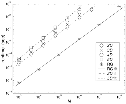
Figure 9: The runtimes (on a 400MHz SUN) of the algorithms used in Sections 2 and 4. The straight lines indicate $t\sim N^{\beta}$, where $\beta=1.2$ in $2D$, $\beta=1.33$ in $5D$ and $\beta=1.15$ in random graphs (RG).

Obviously, a trade-off in Step 2 is involved when choosing the number of small boxes.

Being the most time consuming part of the algorithm, Step 3 is the main contributor when deciding how the runtime depends on $N$. The runtimes for most of our runs are shown in Fig. 9. We see that the runtime is $O(N^{\beta})$, where $\beta\approx 1.3$, resulting in ‘feasible’ runtimes for graphs with up to $N>4\cdot 10^{6}$. Note that the runtime of the much simpler algorithm used on random graphs also grows like a power-law with $\beta=1.15$, even though the number of operations is clearly $O(N)$. In fact, the number of comparisons with potential neighbours per vertex is very nearly constant in our implementation, i.e. the total number of neighbour tests is $O(N)$ in RGGs as well. Of course, this is only possible if the number of subboxes also increases with $N$. Managing the partitioning part of the algorithm adds to the runtime. To sum up, the power-law increase in the runtime illustrated in Fig. 9 for both random graphs and RGGs is probably mainly due to cache misses. The slightly higher values of $\beta$ in the RGGs stems from the additional time used when partitioning the $d$-dimensional box into smaller boxes.

Step 4 is worth a comment. When running the algorithm we are interested in information at certain values of $\alpha$. Instead of generating a new graph for every data point needed, we first set up the graph with the minimal connectivity we want to look at. This is easily accomplished with our algorithm. Given an $\alpha$-window $[\alpha_{min},\alpha_{max}]$ in which we want to examine the graph, we find all the edges belonging to the graph when $\alpha=\alpha_{max}$, but we only add the edges corresponding to $\alpha=\alpha_{min}$. The rest of the edges, those who are to be added when $\alpha$ is gradually increased to $\alpha_{max}$, are stored in a priority queue. It is then a simple task to increase $\alpha$ as one wishes. As mentioned earlier, in Figs. 4 and 5 each curve is based upon 300 data points, i.e. $\Delta\alpha=0.005$.

The source code, written in C, is available upon request. For a more accurate and technical discussion of fast algorithms in relation to RGGs, see e.g. [47].

6 Summary

In this paper we have illustrated the usefulness of random geometric graphs in network theory and how to implement them efficiently. Several properties of random geometric graphs in the vicinity of the critical connectivity $\alpha_{c}$ have been analysed. We have determined the size of the largest cluster numerically and shown that $\alpha_{c}(d)$ approaches $\alpha_{c}(\infty)=1$ found in random graphs in a power-law fashion. We have verified that the distribution of cluster sizes is cut in two just when the connectivity becomes larger than $\alpha_{c}$. Interestingly, the derivation of the cluster coefficient shows that, even in the limit of infinite dimensionality $d$, random geometric graphs are not identical to random graphs.

Random geometric graphs share properties with both lattice models and standard random graphs. Random geometric graphs allow us to work with random graphs with a local structure. In addition, it is straightforward to add ‘long’ edges if one wishes to simulate, e.g., a small world network. With all this in mind, we hope this paper will make random geometric graphs more widely used in network theory.

Appendix A Derivation of $C_{d}$

In order to determine the cluster coefficient for arbitrary $d$, one must find the fractional overlap $\rho_{d}$. Since $\rho_{d}$ has no angular dependence, Eq. (10) reduces to

$$C_{d}=\frac{d}{R^{d}}\int_{0}^{R}\rho_{d}(r)r^{d-1}\textrm{d}r.$$ (18)

Since $\rho_{1}=1-\frac{r}{2R}$, $C_{1}=\frac{3}{4}$. From Fig. 10 we see that in $2D$ the overlapping area—the area circumscribed by the fat lines—is $2(A-B)$, where $A$ is the area of the part of the circle swept out by the angle $\theta=2\arccos(r/2R)$ between the two dashed lines originating from the center of the lowest circle, and $B$ is the area of the dashed triangle. Now, $A=\frac{1}{2}\theta R^{2}$ and $B=R^{2}\cos(\theta/2)\sin(\theta/2)=\frac{1}{2}R^{2}\sin\theta$. The area of the overlap is then $R^{2}(\theta-\sin\theta)$, so $\rho_{2}=\frac{1}{\pi}(\theta-\sin\theta)$ and $C_{2}=1\!-\!\frac{3\sqrt{3}}{4\pi}.$

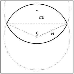
Figure 10: Determination of the cluster coefficient $C$, which in $2D$ is equal to the average fractional area overlap of the two circles. $R$ is the radius of the circles and $r$ the distance between their centers. The area of the overlap is confined within the fat arcs originating from the two circles (dotted). The dashed lines are helpful in the derivation of the overlap—see the text.

For $d\geq 3$, the use of cylindrical coordinates and the relation

$$2\pi\prod_{i=2}^{n-1}\int_{0}^{\pi}\sin^{n-i}\theta_{i}\textrm{d}\theta_{i}=\frac{n\pi^{n/2}}{\Gamma(\frac{n+2}{2})}$$ (19)

results in

$$\rho_{d}(r)=\frac{2}{\sqrt{\pi}}\frac{\Gamma(\frac{d+2}{2})}{\Gamma(\frac{d+1}{2})}\int_{0}^{\arccos(\frac{r}{2R})}\sin^{d}\theta\textrm{d}\theta.$$ (20)

By reversing the integration in $C_{d}$ we get

$$C_{d}=\frac{3}{\sqrt{\pi}}\frac{\Gamma(\frac{d+2}{2})}{\Gamma(\frac{d+1}{2})}\int_{0}^{\frac{\pi}{3}}\sin^{d}\theta\textrm{d}\theta,$$ (21)

which can be solved by integration by parts. The use of the duplicate formula for the Gamma function then finally leads to Eq. (11).

For large $d$, the ratio of the Gamma functions in Eq. (21) is given by Stirling’s approximation. By putting $x=\cos\theta-1/2$, the cluster coefficient can therefore be written as

$$C_{d}\simeq\sqrt{\frac{6d}{\pi}}\!\left(\frac{3}{4}\right)^{\frac{d}{2}}\!\!\int_{0}^{\frac{1}{2}}\!\exp\left[\frac{d\!-\!1}{2}\ln f(x)\right]\!\textrm{d}x,$$ (22)

where $f(x)=1-\frac{4x}{3}(1+x)$. Since the contributions to the integral for large $d$ are significant only when $x\simeq 0$, $\ln f$ can be expanded to 1st order and Eq. (13) is recovered.

Acknowledgements

We thank J. Neil Bearden, Stefan Boettcher and Paolo Sibani for helpful comments. We are especially indebted to Allon Percus for very valuable discussions and correspondence. This work was financially supported by Statens Naturvidenskabelige Forskningsråd.

References

- [1] Albert-László Barabási and Réka Albert. Statistical mechanics of complex networks. cond-mat/0106096v1, pages 1–54, 2001.
- [2] Steven H. Strogatz. Exploring complex networks. Nature, 410:268–276, 2001.
- [3] Bernardo A. Huberman. Growth dynamics of the World-Wide Web. Nature, 401:131, 1999.
- [4] M. E. J. Newman, S.H. Strogatz, and D.J. Watts. Random graphs with arbitrary degree distributions and their applications. Physical Review E, 64:026118, 2001.
- [5] Réka Albert and Albert-László Barabási. Emergence of scaling in random networks. Science, 286:509–512, 1999.
- [6] M. E. J. Newman. Clustering and preferential attachment in growing networks. Physical Review E, 64:025102, 2001.
- [7] L. A. N. Amaral, A. Scala, M. Barthélémy, and H. E. Stanley. Classes of small-world networks. Proc. Natl. Acad. Sci. USA, 97:11149–11152, 2000.
- [8] Duncan J. Watts and Steven H. Strogatz. Collective dynamics of ‘small-world’ networks. Nature, 393:440–442, 1998.
- [9] Stuart Kauffman. At Home in the Universe. Oxford University Press, 1995.
- [10] P. Erdös and A. Rényi. On the evolution of random graphs. Publ. Math. Inst. Hung. Acad. Sci., 5:17–61, 1960.
- [11] Duncan S. Callaway, John E. Hopcroft, Jon M. Kleinberg, M. E. J. Newman, and Steven H. Strogatz. Are randomly grown graphs really random? Physical Review E, 64:041902, 2001.
- [12] Béla Bollobás. Random Graphs. Academic Press, 1985.
- [13] Scott Kirkpatrick and Bart Selman. Critical behavior in the satisfiability of random boolean expressions. Science, 264:1297–1301, 1994.
- [14] Jon M. Kleinberg. Navigation in a small world. Nature, 406:845, 2000.
- [15] D. Stauffer and A. Ahorony. Introduction to Percolation Theory. Taylor and Francis, 1992.
- [16] Reuven Cohen, Keren Erez, Daniel ben Avraham, and Shlomo Havlin. Resilience of the Internet to Random Breakdowns. Physical Review Letters, 85:4626–4628, 2000.
- [17] Réka Albert, Hawoong Jeong, and Albert-László Barabási. Error and attack tolerance of complex networks. Nature, 406:378–382, 2000.
- [18] P. L. Krapivsky, S. Redner, and F. Leyvraz. Connectivity of Growing Random Networks. Physical Review Letters, 85:4629–4632, 2000.
- [19] Réka Albert and Albert-László Barabási. Topology of Evolving Networks: Local Events and Universality. Physical Review Letters, 85:5234–5237, 2000.
- [20] S. N. Dorogovtsev and J. F. F. Mendes. Evolution of networks with aging of sites. Physical Review E, 62:1842–1845, 2000.
- [21] D. J. Watts. Small Worlds. Princeton University Press, 1999.
- [22] M. E. J. Newman and D. J. Watts. Scaling and percolation in the small-world network model. Physical Review E, 60:7332–7342, 1999.
- [23] M. E. J. Newman. Models of the small world. Journal of Statistical Physics, 101:819–841, 2000.
- [24] Jayanth R. Banavar, Amos Maritan, and Andrea Rinaldo. Size and form in efficient transportation networks. Nature, 399:130–132, 1999.
- [25] W. Xia and M. F. Thorpe. Percolation properties of random ellipses. Physical Review A, 38(5):2650–2656, 1988.
- [26] I. Balberg. ”Universal” percolation-threshold limits in the continuum. Physical Review B, 31:4053–4055, 1985.
- [27] U. Alon, A. Drory, and I. Balberg. Systematic derivation of percolation thresholds in continuum systems. Physical Review A, 42:4634–4638, 1990.
- [28] U. Alon, I. Balberg, and A. Drory. New, heuristic, percolation criterion for continuum systems. Physical Review Letters, 66:2879–2882, 1991.
- [29] J. Quantanilla, S. Torquato, and R. M. Ziff. Efficient measurements of the percolation threshold for fully penetrable disks. Journal of Physics A: Math. Gen., 33:L399–L407, 2000.
- [30] I. Balberg. Recent developments in continuum percolation. Phil. Mag. B, 56(6):991–1003, 1987.
- [31] Philippe Jund, Rémi Jullien, and Ian Campbell. Random walks on fractals and stretched exponential relaxation. Physical Review E, 63:036131, 2001.
- [32] Romualdo Pastor-Satorras and Alessandro Vespignani. Epidemic Spreading in Scale-Free Networks. Physical Review Letters, 86:3200–3203, 2001.
- [33] Peter Cheeseman, Bob Kanefsky, and William M. Taylor. Where the Really Hard Problems Are. Proc. of IJCAI-91, pages 331–337, 1991.
- [34] Philip W. Anderson. Solving problems in finite time. Nature, 400:115–116, 1999.
- [35] K. Y. M. Wong and D. Sherringham. Graph bipartitioning and spin glasses on a random network of fixed finite valence. Journal of Physics A: Math. Gen., 20:L793–L799, 1987.
- [36] Michael Molloy and Bruce Reed. A Critical Point for Random Graphs with a Given Degree Sequence. Random Structures and Algorithms, 6:161–179, 1995.
- [37] Michael Molloy and Bruce Reed. The Size of the Giant Component of a Random Graph with a Given Degree Sequence. Combinatorics, Probability and Computing, 7:295–305, 1998.
- [38] M. D. Rintoul and S. Torquato. Precise determination of the critical threshold and exponents in a three-dimensional continuum percolation model. Journal of Physics A: Math. Gen., 30:L585–L592, 1997.
- [39] Edward T Gawlinski and H Eugene Stanley. Continuum percolation in two dimensions: Monte Carlo tests of scaling and universality for non-interacting discs. Journal of Physics A: Math. Gen., 14:L291–L299, 1981.
- [40] Salvatore Torquato. Random Heterogenouos Materials: Microstructure and Macroscopic Properties. Springer, 2002.
- [41] David S. Johnson et. al. Optimization by simulated annealing: An experimental evaluation; part 1, graph bi-partitioning. Operations Research, 37:865–892, 1989.
- [42] Peter Merz and Bernd Freisleben. Memetic algorithms and the fitness landscape of the graph bi-partitioning problem. Lecture Notes in Computer Science, 1498:765–774, 1998.
- [43] Stefan Boettcher and Allon G. Percus. Nature’s way of optimizing. Artificial Intelligence, 64:275–286, 2000.
- [44] Stefan Boettcher and Allon G. Percus. Extremal optimization for graph partitioning. Physical Review E, 64:026114, 2001.
- [45] Stefan Boettcher and Allon G. Percus. Extremal optimization: Methods derived from co-evolution. GECCO-99: Proceedings of the Genetic and Evolutionary Computation Conference, pages 825–832, 1999.
- [46] Stefan Boettcher. Extremal optimization of graph partitioning at the percolation threshold. Journal of Physics A: Math. Gen., 32:5201–5211, 1999.
- [47] Matthew T. Dickerson and David Eppstein. Algorithms for Proximity Problems in Higher Dimensions. Comp. Geom. Theory and Appl., 5:277–291, 1996.