Birth and long-time stabilization of out-of-equilibrium coherent structures

Abstract

We study an analytically tractable model with long-range interactions for which an out-of-equilibrium very long-lived coherent structure spontaneously appears. The dynamics of this model is indeed very peculiar: a bicluster forms at low energy and is stable for very long time, contrary to statistical mechanics predictions. We first explain the onset of the structure, by approximating the short time dynamics with a forced Burgers equation. The emergence of the bicluster is the signature of the shock waves present in the associated hydrodynamical equations. The striking quantitative agreement with the dynamics of the particles fully confirms this procedure. We then show that a very fast timescale can be singled out from a slower motion. This enables us to use an adiabatic approximation to derive an effective Hamiltonian that describes very well the long time dynamics. We then get an explanation of the very long time stability of the bicluster: this out-of-equilibrium state corresponds to a statistical equilibrium of an effective mean-field dynamics.
Keywords:
Statistical ensembles. Long-range interactions. Mean-field models. Classical rotators. XY model.

1 Introduction

The Hamiltonian Mean Field model (HMF) has attracted much attention in the recent years as a toy model to study the dynamics of systems with long-range interactions, and its relation to thermodynamics Antoni ; AnteneodoTsallis ; LatoraRapisardaRuffo . The HMF model describes an assembly of $N$ fully coupled rotators, whose Hamiltonian is:

$$H = \sum_{i=1}^{N}\frac{p_{i}^{2}}{2}+\frac{c}{2N}\sum_{i,j=1}^{N}\cos(\theta_{i}-\theta_{j})\quad,$$ (1)

where $\theta_{i}$ is the angle of the $i$-th planar rotator with a fixed axis. As the interaction only depends on the angles of the rotators, this model can alternatively be viewed as representing particles that move on a circle, whose positions are given by the $\theta_{i}$ and interact via an infinite-range force. If $c$ is negative, the interaction among rotators is ferromagnetic, corresponding to an attractive interaction among particles. When $c$ is positive, the interaction among rotators is antiferromagnetic and repulsive in the particle interpretation. In this article, we will focus our study on this latter case, and put $c=1$.

As first noticed in Ref. Antoni , this model has a very interesting dynamical behavior. In contrast to the statistical mechanics predictions, a bicluster forms at low energy (see Fig. 1), for a special, but wide class of initial conditions: it appears as soon as the initial velocity dispersion of the particles is small, for any initial spatial distribution. This clustering phenomenon and its unexpected dependence on initial conditions were precisely studied in Ref. drh , but remained essentially unexplained. Several details of the dynamics were numerically studied and it has been in particular emphasized that the energy temperature relation is modified: although still linear, the slope in the molecular dynamics simulations is different from the theoretical prediction. No sign in the numerics was found of the decay to the constant density profile predicted by the canonical ensemble. On the contrary, recently performed simulations FFR with a smaller number of particles have shown a long-time degradation of the bicluster, suggesting its transient non-equilibrium nature. The question of the time asymptotic stability of the bicluster, in the limit of an infinite number of particles, remains however open and will be discussed in the conclusions.

We will consider in this work two different theoretical approaches that lead to an analytical explanation of the clustering process and of the long time stability of the structure. In section 2, in order to explain the short time bicluster formation, we first propose a hydrodynamical description that links Hamiltonian (1) to a forced Burgers equation (these results were shortly presented in a previous brief note BDR ). This striking phenomenon is then described in Lagrangian coordinates, giving rise to intersections of trajectories and formation of high (or even infinite) particle densities. We then solve in section 3 this equation, using extensively the method of characteristics. Beyond the theoretical interest in such structures for Hamiltonian systems, we will show some connections of this problem with other subjects; namely, active transport in hydrodynamics, and the formation of caustics in the flow of the associated Burgers equation.

Section 4 presents the second approach, which is particularly powerful for explaining the long-time evolution of the bicluster. The dynamics involves two well separated time-scales. Using a variational approach, we will show how to construct an effective Hamiltonian where all the fast oscillations are averaged out. Not only this effective dynamics accurately represents the one of the original Hamiltonian but, in addition, the complete statistical thermodynamics can be easily derived in the microcanonical and canonical ensembles. It predicts the existence of the bicluster as an equilibrium state, with the correct density profile and the microcanonical temperature energy relation found in the numerical experiments of Ref. drh . The long lifetime of these out-of-equilibrium states can therefore be interpreted by the fact that they appear as equilibrium states of an effective Hamiltonian representing the long-time motion. Section 5 is devoted to some conclusions and perspectives of future developments.

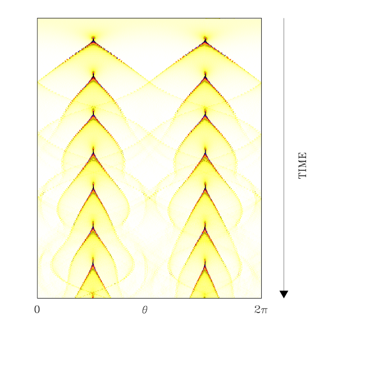
Figure 1: Bicluster formation : short-time evolution of the particle density in grey scale: the darker the grey, the higher the density. Starting from an initial condition with all the particles evenly distributed on the circle, one observes a very rapid concentration of particles, followed by the quasi periodic appearance of “chevrons”, that shrink as time increases.

2 Hydrodynamical description at zero temperature

2.1 Introduction

To describe the initial clustering process, we consider the associated Vlasov equation, which can be rigorously derived in the thermodynamic limit $N\longrightarrow\infty$ Kinlimit ; BraunHepp . Denoting by $f(\theta,p,t)$ the one particle distribution function, we have:

$$\frac{\partial f}{\partial t}+p\frac{\partial f}{\partial\theta}-\left[\frac{1}{2\pi}\int_{-\infty}^{+\infty}du\int_{0}^{2\pi}d\alpha\ f(\alpha,u,t)\sin(\theta-\alpha)\right]\frac{\partial f}{\partial p}=0$$ (2)

Let us define as follows, a density

$$\rho(\theta,t)=\int_{-\infty}^{+\infty}f(\theta,p,t)\;dp$$ (3)

and a velocity field

$$\rho(\theta,t)v(\theta,t)=\int_{-\infty}^{+\infty}pf(\theta,p,t)\;dp\quad.$$ (4)

As the numerical simulations reported in Ref. drh have shown that the bicluster appears when the velocity dispersion is small, we will consider here the zero temperature approximation, i.e. we neglect the velocity dispersion and consider the ansatz $f(\theta,p,t)=\rho(\theta,t)\delta(p-v(\theta,t))$, where $\delta$ refers to the Dirac function. The Vlasov equation (2) can consequently be simplified to

$$\frac{\partial f}{\partial t}+p\frac{\partial f}{\partial\theta}-F(\theta,t)\;\frac{\partial f}{\partial p}=0$$ (5)

where one notes

$$F(\theta,t)=\frac{1}{2\pi}\int_{0}^{2\pi}d\alpha\ \rho(\alpha,t)\sin(\theta-\alpha)\quad.$$ (6)

The sum of the time derivative of Eq. (3) and the $\theta$-derivative of Eq. (4), leads to

$$\frac{\partial\rho}{\partial t}+\frac{\partial(\rho v)}{\partial\theta} = \int_{-\infty}^{+\infty}\left(\frac{\partial f}{\partial t}+p\frac{\partial f}{\partial\theta}\right)dp$$ (7)

$$= \int_{-\infty}^{+\infty}dp\ F(\theta,t)\frac{\partial f}{\partial p}=0\quad.$$

We obtain therefore the equation which accounts for mass conservation

$$\frac{\partial\rho}{\partial t}+\frac{\partial(\rho v)}{\partial\theta}=0\quad.$$ (8)

Using the time derivative of Eq. (4) and Eq. (8), we obtain

$$\frac{\partial\left(\rho v\right)}{\partial t}=\rho\left(\frac{\partial v}{\partial t}+v\frac{\partial v}{\partial\theta}\right)-\frac{\partial(\rho v^{2})}{\partial\theta}\quad.$$ (9)

However, the time derivative of the left-hand-side gives also

$$\frac{\partial\left(\rho v\right)}{\partial t} = \int_{-\infty}^{+\infty}p\frac{\partial f}{\partial t}\;dp$$ (10)

$$= -\int_{-\infty}^{+\infty}p^{2}\frac{\partial f}{\partial\theta}\;dp+F(\theta,t)\int_{-\infty}^{+\infty}p\frac{\partial f}{\partial p}\;dp$$

$$= -v^{2}\frac{\partial\rho}{\partial\theta}-\rho\frac{\partial v}{\partial\theta}2v+F(\theta,t){\rho}(\theta,t)\quad.$$

Equations (9) and Eq. (10) lead finally to the following Euler equation without pressure term:

$$\frac{\partial v}{\partial t}+v\frac{\partial v}{\partial\theta}=\frac{1}{2\pi}\int_{0}^{2\pi}d\alpha\ \rho(\alpha,t)\sin(\theta-\alpha)$$ (11)

Equations (8) and (11) show that the dynamics of the model at low temperature can be therefore mapped onto an active scalar advection problem.

2.2 Linear analysis

Linearizing equations (8) and (11), by assuming small velocities ($v\ll 1$) and almost uniform density ($\rho=1+\rho_{1}(\theta,t)$ with $\rho_{1}\ll 1$), we are left with:

$$\frac{\partial\rho_{1}}{\partial t}+\frac{\partial v}{\partial\theta}=0$$ (12)

$$\frac{\partial v}{\partial t}=\frac{1}{2\pi}\int_{0}^{2\pi}\rho_{1}(\alpha,t)\sin(\theta-\alpha)$$ (13)

a system which is easily solved by a spatial Fourier series development. Assuming a zero initial velocity field, we get

$$\rho_{1}(\theta,t)=\sqrt{2}\ \ v_{m}\cos\theta\cos\omega t$$ (14)

$$v(\theta,t)=v_{m}\sin\theta\sin\omega t~{},$$ (15)

where the time-scale of the oscillation is given by the inverse of a sort of “plasma frequency” $\omega=\sqrt{2}/2$, which describes, as in the Poisson-Boltzmann case, the instability of the uniform density state Nicholson . In the attractive case ($c=-1$ in Hamiltonian (1)), this time scale would control the depart from the initial uniform density towards the formation of the density profile of the single cluster that appears at low temperature Ina1 ; Ina2 , in analogy with Jeans instability in gravitational systems Binney .

This linear analysis is, however, not sufficient to explain the formation of the bicluster and we have to carry out a non linear analysis.

2.3 Non linear analysis

This analysis relies on the existence of two time-scales in the system: the first one is intrinsic and corresponds to the inverse of the “plasma frequency” $\omega$; the second one is connected to the energy per particle $e$. When the energy is sufficiently small, these time-scales are very different, and it becomes possible to use averaging methods. The presence of two well separated time-scales also explains, in some sense, the appearance of the bicluster in the low energy limit.

We introduce therefore a long time-scale $\tau=\varepsilon t$, with $\varepsilon=v_{m}/\sqrt{2}=\sqrt{2e}$, and we look for solutions of the following form:

$$v(\theta,t) = v_{m}\sin\theta\sin\omega t+\varepsilon\ u(\theta,\tau)\quad.$$ (16)

In order to evaluate the force on the r.h.s. of Eq. (11) in the nonlinear regime, we will use expressions (14) and (15), given by the linear analysis. Indeed, due to the special form of the Hamiltonian, the force depends only on the first Fourier component of the density. Hence, our hypothesis amounts to assume that the sinusoïdal behavior of the density, found in the linear regime, holds the same in the non-linear regime: the results presented below confirm the validity of this assumption.

In analogy with studies of the wave-particle interaction in plasma physics plasma ; firpo , our system may be seen as a bulk of particles interacting with waves that are sustained by the bulk itself. Here, the wave is created by the small density and velocity oscillations already present in the linear analysis. In the low energy regime, the phase velocity of the wave with the plasma frequency $\omega$ is much higher than the velocities of the bulk particles, causing a very small wave-particle interaction strength: the wave has therefore a very long life-time. This also explains the quality of the linear approximation for the force that we have used in the Euler equation (11).

Introducing expression (16) in Eq. (11), terms to first order in $\varepsilon$ disappear by construction. Order $\varepsilon^{2}$ terms give:

$$\frac{\partial u}{\partial\tau}+u\frac{\partial u}{\partial\theta} + 2\sin\theta\cos\theta\sin^{2}\omega t$$ (17)

$$+ \left(\sin\theta\frac{\partial u}{\partial\theta}+u\cos\theta\right)\sqrt{2}\sin\omega t=0$$

Averaging over the short time scale $t$, we obtain:

$$\frac{\partial u}{\partial\tau}+u\frac{\partial u}{\partial\theta} = -\frac{1}{2}\sin 2\theta$$ (18)

which is a spatially forced Burgers equation without viscosity, describing the motion of fluid particles in the potential $V(\theta)=1/4\,\cos 2\theta$.

The Burgers equation has been studied in many different contexts by mathematicians interested in a pressureless description of fluid motion, and by physicists in the context of ballistic aggregation models young . In particular, the forced Burgers equation has been very carefully studied from a mathematical viewpoint moserjauslin . Cosmologists have proposed a very interesting adhesion model that uses Burgers-like equations to explain structure formation in the universe youngIHP . Moreover, this equation may be also viewed as a nice model of active transport of the vorticity field in fluid mechanics Castillo .

A well known property of the Burgers equation without viscosity, is that the solution becomes multi-stream after a finite time: the appearance of shocks (see Fig. 2) in the velocity profile $u(\theta)$ corresponds to the creation of singularities in the density profile (see Fig. 3). This is a consequence of the two main assumptions: the medium is supposed to be continuous and the temperature is set at zero. Weakening either assumption would have smoothed out the singularities. In the original discrete Hamiltonian model, particles can cross and, after some time, those that travel faster can be catched by the slower ones that lie downstream, creating the spiral dynamics exemplified in Fig. (4). The particle density has a peak at the center of the spiral (Fig. 3), and diverges at the peak position in the $N\to\infty$ limit at the shock time $\tau_{s}$. The presence of a shock at finite time in the forced Burgers equation does not prevent the hydrodynamical description from remaining valid at longer times, when, moreover, several repeated shocks are observed at regular time intervals. We will indeed show that it can adequately describe even the long-time evolution. In addition, let us remark that it’s the double well shape of the potential that forces the Burgers equation, which is responsible for the formation of two clusters. Starting from the initially uniform state, the particles will move around the bottom of the both wells and the majority of them happen to be there at the same time at the shock time, creating therefore two coherent structures that after several oscillations form the bicluster at long-time.

Figure 2: Shock Dynamics. Phase space portrait of $N=10^{4}$ particles, which at $\tau=\sqrt{2e}t=0$ are uniformly distributed in space (dotted line) with a small sinusoidal velocity profile, not visible in the figure. The resulting energy is $e=6.7\ 10^{-4}$. Velocity profiles $u(\theta)$ are then shown at $\tau=\pi/4$ (dashed line), $\tau=3\pi/8$ (dashed-dotted line) and $\tau=\tau_{s}=\pi/2$, the first shock time (solid line). Only half the space is shown since the curves are $\pi$-periodic.

Figure 3: Particle density $\rho(\theta)$ at $\tau=0$ (dotted line), $\tau=\pi/4$ (dashed line), $\tau=3\pi/8$ (dashed-dotted line) and $\tau=\tau_{s}=\pi/2$ (solid line). The initial condition is the same as in Fig. 2. We clearly see the appearance of one of the two density peaks of the bicluster.

Figure 4: Spiral Dynamics. Phase space portrait of $N=10^{4}$ particles at $\tau=500$. The initial condition is the same as in Fig. 2.

3 Solution of the spatially forced Burgers equation by the method of characteristics

The method of characteristics is the appropriate mathematical tool to study more quantitatively the forced Burgers equation (18), but it has also a direct physical meaning: the characteristics correspond to the Lagrangian trajectories of the Euler equation, and are therefore good approximations for the particle trajectories of the finite $N$ Hamiltonian system (1) when $N\gg 1$.

Figure 5: Panel (a) presents the characteristics of equation (18) whereas panel (b) presents the trajectories of the particles of the Hamiltonian (1) with the same initial condition as in Fig. 2. One can see the three first appearances of the “chevrons”. Two phenomena are not captured by the characteristics: the small oscillations of the real trajectories, which are averaged out, and the presence of untrapped particles, close to the saddle-points of the effective $\cos 2\theta$ potential.

In the case of unidirectional nonlinear wave motions, the method is standard and proceeds as indicated, for example, in Ref. Zauderer . We obtain in this case the following pendulum equation for the characteristics $\theta(\tau)$:

$$\frac{d^{2}\theta}{d\tau^{2}}+\frac{1}{2}\sin 2\theta = 0~{},$$ (19)

with the initial conditions $\theta(0)=\theta_{0}$ and $\dot{\theta}(0)=0$. The solution of the above equation can be easily derived lawden and reads:

$$\theta=\arcsin\left[\sin\theta_{0}\ \mbox{sn}\left(\tau+K_{0},\sin\theta_{0}\right)\right]$$ (20)

where $K_{0}=K(\sin\theta_{0})$, $K$ is the complete elliptic integral of the 1st kind and sn, the elliptic sine function. Fig. (5a) shows the characteristics, i.e. the solutions of Eq. (19) corresponding to different initial conditions $\theta_{0}$ evenly distributed in $[0,2\pi]$ at $t=0$ and with zero initial velocity. One clearly sees their oscillatory behavior inside one of the two wells of the effective potential $\cos 2\theta$, located at $\theta=0$, with a period $4K_{0}$ which strongly depends on the initial position. Fig. (5a) emphasizes also that the characteristics cross themselves, and the associated caustics are responsible for the enhancement of the particle density field that forms the “chevrons”. The time of the first divergence in the density $\tau_{s}$ is the time of the first characteristic crossing and also the time of the first shock in the velocity profile. The particles performing a quasi-harmonic oscillatory motion in the bottom of the well are the ones with shorter periods. The shortest period is obtained in the harmonic limit $4K(0)=2\pi$, leading to $\tau_{s}=\pi/2$ for the time of appearance of the first shock. In the original units, it reads

$$t_{s}=\frac{\tau_{s}}{\varepsilon}=\frac{\pi}{\sqrt{8e}}\quad.$$ (21)

This shock results in a singularity in Eulerian space at the corresponding time. However this singularity disappears immediately after forming and two singularities of another kind arise in its place, which are the boundaries of the three streams region. The chevron is their manifestation in the density profile. The shock time singularity is called $A_{3}$ in Arnold’s classification arnold ; Zeldovich while the “chevrons” singularity is of $A_{2}$ type. The latter is the boundary of structures and can exist at any moment of time, whereas the former exist only when a chevron originates. The recurrence time for the appearance of chevrons is $t_{n}=t_{s}*(2n-1)$ and the comparison with the numerics shows a very good agreement.

Figs. (5a) and  (5b) show that the agreement is really good not only at the qualitative but also at the quantitative level. Only two features are missed by the Lagrangian description. The fast oscillations of very small amplitude, already hardly visible in Fig. (5b) is of course totally absent in the characteristics because of the averaging procedure used to get Eq. (18). One can also easily show that the amplitude of this fast oscillation is rapidly decreasing with the increase of the number of particles and is vanishingly small for $N\to\infty$. The second point is the presence of untrapped particles in Fig. (5b), which is a direct consequence of the oscillations of the height of the potential barriers. This effect is important only for highly energetic particles whose trajectories in phase space are closed to the separatrix of the Kelvin’s cat eye of Fig. (4). However, as we will show in the next section, these particles do not take part to the creation of caustics (i.e. of the chevrons of Fig. 1) which are generated only by the particles close to the bottom of the wells.

3.1 The chevrons as caustics of the characteristics

We will now explain the shape of the ”chevrons” (Fig. 1), which correspond to zones of infinite density i.e. to the envelops of the characteristics, the so-called caustics. The family of the characteristics is defined by

$$F(\tau,\theta,\theta_{0})=\sin\theta(\tau,\theta_{0})-\sin(\theta)=0$$ (22)

in the plane $(\theta,\tau)$ with the parameter $\theta_{0}$. The envelope of this family would then be defined by the two following equations

$$F(\tau,\theta,\theta_{0}) = 0$$ (23)

$$\frac{\partial F}{\partial\theta_{0}}(\tau,\theta,\theta_{0}) = 0$$ (24)

However, it is not possible to extract $\theta_{0}$ as a function of $\theta$ and $\tau$ from Eq. (24), in order to obtain a closed expression $F(\tau,\theta,\theta_{0}(\tau,\theta))$ for the caustics. We will use approximate expressions of $F$ close to the shocks.

In the neighborhood of the shock, the trajectories can be approximated by straight lines, with the following expression:

$$\theta(\tau,\theta_{0}) = v_{0}\left(\tau-K_{0}\right)$$ (25)

where $v_{0}=v(K_{0})$ is the speed of the particle at the bottom of the potential well.

The envelope of this family of characteristics can then be obtained Zauderer by solving the following system of equations

$$\theta(\tau,\theta_{0}) = v_{0}\left(\tau-K_{0}\right)$$ (26)

$$0 = v_{0}^{{}^{\prime}}\left(\tau-K_{0}\right)-v_{0}K^{{}^{\prime}}_{0}$$ (27)

where the primes denotes the derivative with respect to $\theta_{0}$. Using the conservation of energy, we easily get $v_{0}=-\sin{\theta_{0}}$ and we obtain thus

$$\tau = \tan{\theta_{0}}\ K^{{}^{\prime}}_{0}+K_{0}$$ (28)

$$\theta = -\displaystyle\frac{\sin^{2}\theta_{0}}{\cos\theta_{0}}\ K^{{}^{\prime}}_{0}\quad.$$ (29)

It is however possible to go further by using higher order terms in the expression of $\theta$ given in Eq. (25), i.e. by considering curves rather than simply straight lines. We have thus

$$\theta(\tau,\theta_{0}) = \theta(K_{0})+\frac{d\theta}{d\tau}_{|K_{0}}\left(\tau-K_{0}\right)+\frac{1}{2}\frac{d^{2}\theta}{d\tau^{2}}_{|K_{0}}\left(\tau-K_{0}\right)^{2}$$ (30)

$$\hskip 56.9055pt+\frac{1}{6}\frac{d^{3}\theta}{d\tau^{3}}_{|K_{0}}\left(\tau-K_{0}\right)^{3}+\dots$$

$$= v_{0}\left(\tau-K_{0}\right)-\frac{v_{0}}{6}\left(\tau-K_{0}\right)^{3}+\dots$$ (31)

where we have replaced in Eq. (31) the derivatives by their expressions. Let us note in particular, that all derivatives of even order will vanish because of the parity property of $\theta$. Using the development of $K_{0}$ at the same order, we finally end with the next order approximation for the caustics

$$\tau = \tau_{s}+3a\theta_{0}^{2}+\left(5b+\frac{2a}{3}\right)\theta_{0}^{4}$$ (32)

$$+\left(7c+\frac{4b}{3}+\frac{4a}{15}-\frac{8a^{3}}{3}\right)\theta_{0}^{6}+O(\theta_{0}^{8})$$

$$\theta = 2a\theta_{0}^{3}+\left(4b+\frac{a}{3}\right)\theta_{0}^{5}$$ (33)

$$+\left(6c+\frac{2b}{3}+\frac{31a}{180}-4a^{3}\right)\theta_{0}^{7}+O(\theta_{0}^{9})$$

where $(a,b,c)=\frac{\pi}{8}\left(1,\frac{11}{48},\frac{173}{2880}\right)$.

Figure 6: Superposition of the caustics over the characteristics of 50 particles evenly distributed between $-\pi/2$ and $\pi/2$ at $t=0$. The analytical formula for the “chevrons” (Eq. 32 and Eq. 33) is superimposed (bold curves). The vertical dashed lines shows the appearance time of the chevrons $t_{n}=t_{s}*(2n-1)$.

It is possible to see in Fig. (6) that the agreement is excellent and that this procedure is really accurate to describe the first chevron. Moreover, one can check that because of the non isochronism of the oscillations, the more energetic particles arrive too late in the bottom of the well to take part to the creation of the caustics, i.e. the singularity in the density space. Consequently, the untrapped particles of the real dynamics, visible in Fig. (5b), but absent of the averaged dynamics of the associated Burgers equation (see Fig. 5a), are irrelevant and do not affect the dynamics of the caustic formation.

This is confirmed by Fig. (7) where the caustics determined by the Burgers’ approach are superimposed on the real trajectories: the shape of the chevrons is very well described. However, the time occurrence of the shock was reduced by a factor 0.84. The reason, clarified in the next section, is due to the renormalization of the oscillation frequency $\omega$ which modifies the oscillation period of the particles. As shown below using a self-consistent procedure, $\omega$ is reduced with respect to the plasma frequency $\omega_{p}$. As the potential height is inversely proportional to $\omega$ this leads therefore to a faster appearance of the shocks.

Figure 7: Superposition of the caustics over the trajectories of 100 particles evenly distributed between 0 and $2\pi$ at $t=0$ for an energy $e=3\ 10^{-6}$. The time occurrence of the shocks was reduced by a factor 0.84 (see text).

As already mentioned, the time occurrence of the $n$th shock is $\tau_{n}(\theta_{0})=(2n-1)\tau_{s}$ which means that its shape will be obtained simply by replacing in Eq. (26) $K_{0}$ by $(2n-1)K_{0}$. Therefore, the lowest order approximation of the $n$th shocks is

$$\theta = 2a(2n-1)\left(\frac{\tau-\tau_{n}}{3a(2n-1)}\right)^{3/2}$$ (34)

$$\theta \propto \frac{\left(t-(2n-1)t_{s}\right)^{3/2}}{\sqrt{2n-1}}$$ (35)

where $n$ is the number of appearance of the ”chevron”. The $1/\sqrt{n}$ factor accounts for the shrinking of the “chevrons” and the bolded line in Fig. (6) attests that this expression is particularly accurate.

Similar caustics are encountered in astrophysics, to explain the large scale structure of the universe: clusters and super clusters of galaxies are believed to be reminiscent of three dimensional caustics arising from the evolution of an initially slightly inhomogeneous plasma Vergassola ; Zeldovich .

3.2 Probability distribution

At this point, it would be important to calculate the density distribution in the vicinity of the singularity. For this hydrodynamical approximation, it would be fully determined by the initial conditions, i.e. the initial velocity distribution. Let us recall that we earlier found drh , that the following analytical formula

$${\cal P}(\theta)=\frac{1}{2\pi}\left(1-\log(2|\sin\theta|)\right)$$ (36)

was an excellent approximation (see Fig. 8), even if we didn’t have any theory for its derivation. Here using the Burgers’ approach, let us obtain a similar result.

Along the particle trajectory, one has

$$\dot{\theta}=\sqrt{\frac{\cos 2\theta-\cos 2\theta_{0}}{2}}$$ (37)

The time $dt(\theta)$ spent by a particle close to a position $\theta$ is inversely proportional to its velocity $\dot{\theta}(\theta_{0})$. Therefore the trajectory parametrized by $\theta_{0}$ (and initiated in $\theta_{0}$) gives a contribution to the density

$$\rho_{\theta_{0}}(\theta)d\theta = \frac{dt(\theta)d\theta}{\displaystyle\int_{-\theta_{0}}^{\theta_{0}}dt(\theta)}=\frac{2\sqrt{2}\ d\theta}{T(\theta_{0})\sqrt{{\cos 2\theta-\cos 2\theta_{0}}}}$$ (38)

where $T(\theta_{0})$ is the period of the trajectory. By recalling that the initial distribution is homogeneous in these numerical computations, one obtains the probability density by averaging over the time, the density of characteristics at a fixed position. We obtain:

$$\rho(\theta)\propto\int_{2\theta}^{\pi}{\frac{2\sqrt{2}\ du}{T(u)\sqrt{\cos 2\theta-\cos 2u}}}$$ (39)

for $\theta=[0,\pi/2]$ whereas the whole distribution is obtained by symmetry and $\pi$-periodicity.

Due to the numerous approximations, the agreement for long time is not perfect, but equation (39) gives a good result as shown by Fig. (8). The disagreement is visible in $0$ and $\pi$, i.e. close to the separatrix. Actually, as we will see in the following, the amplitude of the effective potential slightly oscillates; this allows the existence of untrapped particles which smooth the density.

Figure 8: Equilibrium distribution. Comparison between the numerical results (diamonds) and the analytical formula (39) (solid line) in the case $e\simeq 10^{-4}$. The dotted line corresponds to the formula (36).

As a conclusion, this hydrodynamical approach has proved to be very successful, since it explains qualitatively and quantitatively, for short times, the main features of the bicluster formation. Nevertheless, the stability and the long time behavior of the structure is not yet understood: this is the object of the next section.

4 Long time evolution of the bicluster

Since the thermodynamics of the antiferromagnetic HMF model predicts a perfectly homogeneous equilibrium state, the bicluster is a non equilibrium structure. However, its long time stability, as well as the fact that it is reached starting from a variety of initial conditions suggest some statistical explanation.

In addition, we have learned from the previous section that particle motion may be split into two parts: a small amplitude rapid oscillation superimposed to a large amplitude slow motion. The idea is thus to look for an effective Hamiltonian dynamics which would only retain the slow motion, and would be appropriate for a statistical description.

4.1 The fast variables

The complete Lagrangian of the antiferromagnetic HMF being

$$L\left({\theta_{i}},{\dot{\theta_{i}}}\right) = \sum_{i=1}^{N}\frac{\dot{\theta_{i}}^{2}}{2}-\frac{1}{2N}\sum_{i,j}\cos(\theta_{i}-\theta_{j})\quad,$$ (40)

the equations of motion are obtained by minimizing the action $S=\int Ldt$ with respect to the functions $\theta_{i}$. Taking advantage of the two well defined time scales, we introduce the following ansatz:

$$\theta_{i}=\theta_{i}^{0}(\tau)+\varepsilon f_{i}(t,\tau)$$ (41)

where $\tau=\varepsilon t$ and $\varepsilon=\sqrt{2e}$ as already defined in the section (2.3). The $f_{i}$’s represent the small rapid oscillations and the $\theta_{i}^{0}$ the slow variables which we are finally interested in. The idea is then to use a variational approach (least action principle), first to obtain the equations of motion of the fast variables $f_{i}$, and then to reintroduce the solutions into the action. In a second stage, averaging over the fast time $t$, we will obtain a variational principle for the slow variables. This approach, inspired by witham , has the double advantage of allowing to obtain an Hamiltonian system for the slow variables, and the one of exhibiting a natural conservation law for this dynamics (the adiabatic invariant). Appendix A briefly presents the use of method witham for a slowly modulated harmonic oscillator, in order to emphasize its power for a very simple model, away from the rather technical context presented here.

We first notice that since the energy of the system is by definition of order $\varepsilon^{2}$, the sums $1/N\sum\cos\theta_{i}^{0}$ and $1/N\sum\sin\theta_{i}^{0}$, which represent the two components of the magnetization vector in terms of the slow variables $\theta_{i}^{0}$, are of order $\varepsilon$. We thus define

$$\varepsilon M_{1x}^{0} = \frac{1}{N}\sum_{i}\cos{\left(\theta_{i}^{0}+\psi\right)}$$ (42)

$$\varepsilon M_{1y}^{0} = \frac{1}{N}\sum_{i}\sin{\left(\theta_{i}^{0}+\psi\right)}$$ (43)

where the phase $\psi$ $\in[0,\pi]$ is chosen such that the scalar dynamical indicator of the clustering is

$$|M_{2}|=\left|\frac{1}{N}\sum_{i}\exp\left(2i\theta_{i}^{0}\right)\right|=\frac{1}{N}\sum_{i}\cos 2\left(\theta_{i}^{0}+\psi\right).$$ (44)

We now introduce the ansatz (41) into the Lagrangian (40), and develop the cosine up to order $\varepsilon^{2}$, obtaining the new Lagrangian $L_{2}$ that depends on the $\theta_{i}^{0}$’s, the $f_{i}$’s and their time derivatives

$$L_{2} = L_{2}\left({\theta_{i}^{0}},{\frac{d\theta_{i}^{0}}{d\tau}},{f_{i}},{\frac{df_{i}}{dt}}\right)$$ (45)

$$= \frac{\varepsilon^{2}}{2}\sum_{i}\left[\left(\frac{d\theta_{i}^{0}}{d\tau}\right)^{2}+2\frac{d\theta_{i}^{0}}{d\tau}\frac{df_{i}}{dt}+\left(\frac{df_{i}}{dt}\right)^{2}\right]$$

$$- \frac{\varepsilon^{2}N}{2}\Bigl{[}(M^{0}_{1x})^{2}+(M_{1y}^{0})^{2}\Bigr{]}+\frac{\varepsilon}{N}\sum_{i,j}f_{i}\sin{(\theta_{i}^{0}-\theta_{j}^{0})}$$

$$- \frac{\varepsilon^{2}}{2N}\sum_{i,j}f_{i}f_{j}\cos(\theta_{i}^{0}-\theta_{j}^{0})\quad.\quad$$

From this expression, considering $\tau$ as a constant, we write the equations of motion for the fast variables $f_{i}$’s. We get

$$\ddot{f_{i}} =M_{1x}^{0}\sin{\left(\theta_{i}^{0}+\psi\right)} -M_{1y}^{0}\cos{\left(\theta_{i}^{0}+\psi\right)}$$ (46)

$$-\frac{1}{N}\sum_{j}f_{j}\cos\left(\theta_{i}^{0}-\theta_{j}^{0}\right)\quad.\quad$$

This is a linear second order equation, with constant coefficients with respect to the fast time, whose solution thus requires the diagonalization of the $N$x$N$ matrix

$${\mathbf{T}}=\left[T_{ij}\right]=\frac{1}{N}\left[\cos(\theta_{i}^{0}-\theta_{j}^{0})\right]\quad,$$ (47)

which has only two non zero eigenvalues (see Appendix B)

$$\omega_{\pm}^{2}=\frac{1\pm|M_{2}|}{2}\quad.$$ (48)

The eigenvectors corresponding to $\omega_{\pm}^{2}$ are respectively

$${\mathbf{X}_{+}} = \left[\cos(\theta_{i}^{0}+\psi)\right]_{i=1\ldots N}$$ (49)

$${\mathbf{X}_{-}} = \left[\sin(\theta_{i}^{0}+\psi)\right]_{i=1\ldots N}\quad.$$ (50)

The general solution for the $f_{i}$’s is therefore

$$f_{i}(t,\tau) = \left[\sqrt{2}A_{+}\sin(\omega_{+}t+\varphi_{+})-\frac{M_{1y}^{0}}{\omega_{+}^{2}}\right]\cos(\theta_{i}^{0}+\psi)$$ (51)

$$+ \left[\sqrt{2}A_{-}\sin(\omega_{-}t+\varphi_{-})+\frac{M_{1x}^{0}}{\omega_{-}^{2}}\right]\sin(\theta_{i}^{0}+\psi)\quad.\qquad$$

4.2 The slow variables

The previous solution for the $f_{i}$ suggests the following new ansatz

$$f_{i} = \left[\sqrt{2}A_{+}(\tau)\sin(\phi_{+}(t))+a_{+}(\tau)\right]\ \cos(\theta_{i}^{0}+\psi)$$ (52)

$$+ \left[\sqrt{2}A_{-}(\tau)\sin(\phi_{-}(t))+a_{-}(\tau)\right]\ \sin(\theta_{i}^{0}+\psi)$$

where $\phi_{\pm}(t)$ are fast variables, and $d\phi_{\pm}/dt$, $A_{\pm}(\tau)$, and $a_{\pm}(\tau)$ are slow variables. We introduce (52) in the Lagrangian (45), and we average over the fast variables $\phi_{\pm}$. Dropping the $\varepsilon^{2}$ overall factor, the averaged Lagrangian reads

$$L_{eff} = \frac{1}{2}\sum_{i=1}^{N}\left(\frac{d\theta_{i}^{0}}{d\tau}\right)^{2}+\frac{N}{2}\left[A_{+}^{2}\omega_{+}^{2}\dot{\phi}_{+}^{2}+A_{-}^{2}\omega_{-}^{2}\dot{\phi}_{-}^{2}\right]$$ (53)

$$-N\Biggl{[}\frac{{M_{1x}^{0}}^{2}+{M_{1y}^{0}}^{2}}{2}+M_{1y}^{0}a_{+}\ \omega_{+}^{2}-M_{1x}^{0}a_{-}\ \omega_{-}^{2}$$

$$\qquad+\left({A_{+}^{2}}+{a_{+}^{2}}\right)\frac{\omega_{+}^{4}}{2}+\left(A_{-}^{2}+a_{-}^{2}\right)\frac{\omega_{-}^{4}}{2}\Biggr{]}\quad.$$

Due to the averaging, the variables $\phi_{\pm}$ are cyclic, $P_{\pm}$, the conjugate momenta of $\phi_{\pm}$, are conserved quantities. Their expression is

$$P_{\pm}=\frac{\partial L_{eff}}{\partial\dot{\phi}_{\pm}}={NA_{\pm}^{2}\omega_{\pm}^{2}\dot{\phi}_{\pm}}\quad.$$ (54)

As the Lagrangian does not depend on the time derivatives of $A_{+}$, $A_{-}$, $a_{+}$, and $a_{-}$, there is no Legendre transform on these variables and the Hamiltonian reads

$$H_{eff} = P_{+}\dot{\phi}_{+}+P_{-}\dot{\phi}_{-}+\sum_{i=1}^{N}p_{i}\dot{\theta}_{i}^{0}-L_{eff}$$ (56)

$$= \frac{P_{+}^{2}}{2NA_{+}^{2}\omega_{+}^{2}}+\frac{P_{-}^{2}}{2NA_{-}^{2}\omega_{-}^{2}}+\sum_{i=1}^{N}\frac{{p_{i}^{0}}^{2}}{2}$$

$$+N\Biggl{[}\frac{{M_{1x}^{0}}^{2}+{M_{1y}^{0}}^{2}}{2}+M_{1y}^{0}a_{+}\omega_{+}^{2}-M_{1x}^{0}a_{-}\omega_{-}^{2}$$

$$\qquad+\left(A_{+}^{2}+a_{+}^{2}\right)\frac{\omega_{+}^{4}}{2}+\left(A_{-}^{2}+a_{-}^{2}\right)\frac{\omega_{-}^{4}}{2}\Biggr{]}\quad.$$

In the absence of conjugate variables of the amplitudes $A_{\pm}$, the corresponding Hamilton’s equation are simply given, from the least action principle, by $\partial_{A_{\pm}}H_{eff}=0$. Together with the equations (54), this leads to the following expressions for the frequencies

$$\frac{d\phi_{\pm}}{dt} = \omega_{\pm}\quad,$$ (57)

expected of course from the previous study of the matrix ${\mathbf{T}}$, and for the amplitudes

$$A_{\pm}^{2} = \frac{P_{\pm}}{N\omega_{\pm}^{3}}\quad.$$ (58)

Finally, from the equations $\partial_{a_{\pm}}H_{eff}=0$, we find

$$a_{+}=-\frac{M_{1y}^{0}}{\omega_{+}^{2}}\quad\mbox{and}\quad a_{-}=\frac{M_{1x}^{0}}{\omega_{-}^{2}}\quad.$$ (59)

Reintroducing expressions (58) and (59) in the Hamiltonian (56), we end up with the effective Hamiltonian describing the slow motion of the particles

$$H_{eff} = \sum_{i}\frac{{p_{i}^{0}}^{2}}{2}+P_{+}\omega_{+}+P_{-}\omega_{-}\quad.$$ (60)

The evolution of the full system is then approximated by the dynamics of this effective Hamiltonian, the constant $P_{+}$ and $P_{-}$ being determined by the initial conditions. However, a difficulty arises when the two eigenvalues crosses, ie when $|M_{2}|$ becomes $0$. Since $\psi$ is defined as half the phase of the complex number $M_{2x}+iM_{2y}$, it experiences at this point a $\pi/2$ jump, and consequently the eigenvectors $X_{\pm}$ are inverted: this phenomenon of eigenvalue crossing is illustrated by Fig. 9.

Figure 9: The diamonds presents the evolution versus time of the main frequency for $N=200$ particles of the original Hamiltonian (1). We have superimposed not only $\omega_{+}$ (dashed line) and $\omega_{-}$ (solid line) using Eqs. (48), but also the numerically computed $|M_{2}|$ (dotted line). We clearly see the exchange of frequency when $|M_{2}|$ touches zero.

However, in most of the numerical experiments conducted in drh , only one fast frequency, $\omega_{-}$ was excited. From now on, we will therefore concentrate on the case $P_{+}=0$, and will not be concerned by the phenomenon of eigenvalue crossing. Dropping the subscript for $P$, we consider the Hamiltonian

$$H_{eff} = \sum_{i}\frac{{p_{i}^{0}}^{2}}{2}+P\sqrt{\frac{1-|M_{2}|}{2}}$$ (61)

The corresponding equations of motion are

$$\ddot{\theta_{i}} = -\frac{P}{N\sqrt{2}\sqrt{1-|M_{2}|}}\sin{2\left(\theta_{i}+\psi\right)}$$ (62)

which have to be compared with Eq. (19): this is still a pendulum equation, but the potential amplitude, depending now self consistently on the particles motion through $M_{2}$, explains the presence of untrapped particles, shown in Fig. (5b). In addition, we have now the right expression for the frequency of the fast oscillations $\omega=\omega_{-}$, and a new conserved quantity has been identified: the adiabatic invariant $P$. Using Eq. (58), we obtain the $A_{-}(M_{2})$ relation which, together with $\omega(M_{2})$, is perfectly verified by numerical simulation as attested by Fig. 10.

Figure 10: Comparison between the numerical (triangles) and analytical (solid line for $\omega_{-}$ given by Eq. (48)) frequency of oscillations. Comparison between the numerical (circles) and analytical (solid line for Eq. (58)) amplitude $\varepsilon$ of oscillation . $e=3.610^{-5}$ and $t_{\mbox{\tiny max}}=1500$.

The full efficiency of this procedure is that it preserves completely the Hamiltonian structure of the problem, making it well suited for a statistical treatment, presented below. However, it is important to emphasize before, that all fast variables having disappeared, this procedure induces a huge gain (of order $1/\varepsilon$) for numerical simulations. This allows to study accurately the statistics and the dynamics of this effective Hamiltonian up to extremely long times, giving conclusion directly relevant to the original model.

Figure 11: Spacio-temporal evolution of 50 particles. Results given by the original Hamiltonian (1) (resp. effective Hamiltonian (60)) with (resp. without) the fast small oscillations superimposed: they are almost indistinguishable. The initial condition corresponds to particles evenly distributed on the circle and with a sinusoïdally modulated impulsion corresponding to an energy density $e=2.5\ 10^{-5}$ and $\varepsilon=5\ 10^{-3}$.

4.3 Study of the effective Hamiltonian

4.3.1 Statistical mechanics of the effective Hamiltonian

We would like to describe the bicluster as an equilibrium state of the effective Hamiltonian (61). Fortunately, due to the special form of the potential, which depends only on the global variable $|M_{2}|$, the statistical mechanics of the effective Hamiltonian are exactly tractable in the microcanonical ensemble.

There are two conserved quantities: the total energy $E$ and the total angular momentum. As the latter only creates a global rotation of the system totally decoupled from the rest of the dynamics, we can consider the total energy without restriction. The density of states $\Omega(E)$ at a given energy, written as an integral in which the energy is split in two parts, a kinetic and a potential one, has the following expression

$$\Omega(E) = \int dV\>\Omega_{kin}(E-V)\>\Omega_{pot}(V)$$ (63)

$$\propto \int d|M_{2}|\>\Omega_{kin}\left(E-V(|M_{2}|)\right)\>\Omega_{conf}(|M_{2}|)\qquad$$

where the sign $\propto$ accounts for an unimportant constant. $\Omega_{kin}$ (resp. $\Omega_{pot}$) is the density of states corresponding to the kinetic (resp. potential) part of the Hamiltonian, and $\Omega_{conf}$ is the density of angular configuration giving rise to a given $|M_{2}|$: since the potential only depends on $|M_{2}|$, $\Omega_{pot}(V)$ is directly proportional to $\Omega_{conf}(|M_{2}|)$. Their expressions are

$$\Omega_{kin}(E) = \int_{-\infty}^{+\infty}\prod_{i}dp_{i}\ \delta\left(\frac{1}{2}\sum_{i}p_{i}^{2}-E\right)$$ (64)

$$\Omega_{conf}(|M_{2}|) = \int_{0}^{2\pi}\prod_{i}d\theta_{i}\ \delta\left(\frac{1}{N}\left(\sum_{i}\cos 2\theta_{i}\right)^{2}\right.$$ (65)

$$+\frac{1}{N}\left.\left(\sum_{i}\sin 2\theta_{i}\right)^{2}-N|M_{2}|^{2}\right)\quad.$$

Using the classical result for a perfect gas, we obtain

$$\Omega_{kin}(E) = \frac{2\pi^{N/2}}{\Gamma(N/2+1)}\ E^{N/2}\quad.$$ (66)

To compute $\Omega_{conf}(|M_{2}|)$, it is possible to use the inverse Laplace transform of the Dirac delta function

$$\delta(x)=\int_{\Gamma}dp\>e^{px}\quad,$$

where $\Gamma$ is a path in the complex plane running from $\Im(p)=-\infty$ to $\Im(p)=+\infty$. The expression of $\Omega_{conf}$ becomes

$$\Omega_{conf}(|M_{2}|) = \int_{\Gamma}dp\>e^{-Np|M_{2}|^{2}}\int_{0}^{2\pi}\prod_{i}d\theta_{i}\>e^{NpM_{2}^{2}}.\quad$$ (67)

To compute the integral over the angles, we use now the Gaussian (also called Hubbard-Stratanovich) transform

$$e^{Npm^{2}} \propto \int_{-\infty}^{+\infty}du\>e^{-N\frac{u^{2}}{4p}+Nmu}\quad.$$

This decouples the integration over the angles $\theta_{i}$, and we have

$$\Omega_{conf}(|M_{2}|) \propto \int_{\Gamma}dp\>e^{-Np|M_{2}|^{2}}\int du\>dv\>e^{-\frac{N}{4p}(u^{2}+v^{2})}$$ (68)

$$\int_{0}^{2\pi}\prod_{i}d\theta_{i}\>e^{N\sum_{i}u\cos 2\theta_{i}+v\sin 2\theta_{i}}$$

$$\propto \int_{\Gamma}dp\>e^{-Np|M_{2}|^{2}}\int_{0}^{\infty}rdre^{-\frac{Nr^{2}}{4p}}I_{0}(r)^{N}\qquad$$ (69)

where $r$ is the polar radius associated with $u$ and $v$, and $I_{0}$ is the modified Bessel function of order $0$. Using the saddle point method on $p$ and $r$, we have finally

$$\Omega_{conf}(|M_{2}|) \propto e^{-N\left(p^{\ast}|M_{2}|^{2}+\frac{{r^{\ast}}^{2}}{4p^{\ast}}-\ln{I_{0}(r^{\ast})}\right)}$$ (70)

$$= e^{-N\left(2p^{\ast}|M_{2}|^{2}-\ln{I_{0}(r^{\ast})}\right)}$$ (71)

where $p^{\ast}$ and $r^{\ast}$ are implicitly defined by

$$\frac{r^{\ast}}{2p^{\ast}} = \frac{d\>\ln{I_{0}(p)}}{dp}_{|r^{\ast}}$$ (72)

$$\frac{{r^{\ast}}^{2}}{4{p^{\ast}}^{2}} = |M_{2}|^{2}\quad.$$ (73)

Using this result, Eq. (63) may be evaluated once again by the saddle point method, which leads after some simple algebra to the equilibrium value $|M_{2}|^{\ast}$, defined by the following equation

$$r^{\ast}(|M_{2}|^{\ast}) = \frac{1}{4\sqrt{1-|M_{2}|^{\ast}}\left(\displaystyle\frac{\sqrt{2}E}{P}-\sqrt{1-|M_{2}|^{\ast}}\right)}\quad.$$ (74)

As shown by Fig. 12, this equation has only one solution for any ratio $E/P$; this indicates an absence of phase transition. As this solution is non zero, a biclusterization will always take place; nevertheless in the large energy limit the particles are almost free and $|M_{2}|^{\ast}$ goes of course to zero.

Figure 12: Statistical prediction of the dynamical indicator $|M_{2}|$ as a function of the ratio between the energy $E$ and the adiabatic invariant $P$.

Once $|M_{2}|^{\ast}$ is known, it is easy to complete the description of the equilibrium state. The temperature $T$ is given by

$$T = \frac{2}{N}\langle E_{c}\rangle=\frac{2}{N}\left\langle E-P\sqrt{\frac{1-|M_{2}|^{\ast}}{2}}\right\rangle$$ (75)

the distribution of velocities is a Maxwellian with temperature $T$, and the distribution of angles has a gibbsian shape $\rho(\theta)\propto e^{-V(\theta)/T}$ with the potential

$$V(\theta) = \frac{P}{N2\sqrt{2}\sqrt{1-|M_{2}|^{\ast}}}\left(1-\cos(2\theta+2\psi)\right)$$ (76)

This potential is inferred from the equations of motion (62).

4.3.2 Relaxation to equilibrium

We have therefore now a complete description of the statistical equilibrium states of the effective Hamiltonian, governed by long range interactions. It has been noticed by various authors that the dynamics of such systems may sustain long lived metastable states before relaxing to equilibrium Antoni ; AnteneodoTsallis ; Latora1 ; gouda . Before comparing the ”effective equilibrium” with the structure created by the dynamics of the real Hamiltonian, it is thus necessary to study the relaxation to equilibrium. As the relaxation properties of long range interacting systems is in itself an important problem, we will consider them now. We will in addition illustrate which statistical properties of the equilibrium distribution is expected to be observed in the real dynamics, for large $N$ and on time scale reasonable for numerical computations.

Figure 13: Relaxation of the first three even moments $<M_{2n}>$ (time averaged) toward equilibrium according to numerical simulations of the effective Hamiltonian (61). The solid (resp. dotted and dashed) lines corresponds to results for $N=200$ (resp. $N=800$ and $N=3200$) particles. $<M_{2}>$, $<M_{4}>$ and $<M_{6}>$ are represented from top to bottom ($<M_{2n}>$ is a decreasing function of $n$). They converge toward the equilibrium values $M_{2}^{\star}=0.510$, $M_{4}^{\star}=0.144$ and $M_{6}^{\star}=0.028$.

Fig. 13 illustrates the approach to equilibrium of the effective Hamiltonian, for three different particle numbers, with initially immobile and homogeneously distributed particles (this corresponds to the typical initial condition used in the real Hamiltonian in Antoni ; drh for instance). We have represented $<M_{2n}>(\tau)$, the time averages of $M_{2n}$ from initial time $0$ to time $\tau$, for $n$ equal to 2, 4 and 6. Temporal fluctuations are thus not visible. We first observe finite size effects concerning the equilibrium values : for instance $M_{6}$ converges for the small system $N=200$ to a value larger than $M_{6}^{\star}$, the equilibrium value.

More interestingly, we observe also that whereas $|M_{2}|$ quickly reaches its equilibrium value, the relaxation time of the successive moments $|M_{4}|$, $|M_{6}|$ strongly depends on the system size, and presumably diverges with $N$. The actual dependence of the relaxation time of each moment, on the particle number, will not be studied in this paper. It would for instance address the issue of whether non equilibrium distributions may be observed in the thermodynamic limit. Such phenomena have indeed already been observed in other long range interacting systems Latora1 ; Latora2 .

We conclude that for a large, but finite, particle number, the moments of the distribution converge toward their equilibrium values. When $N$ increases, the relaxation time for the high order moments may however be larger than computationally achievable times and, we thus expect the simulation to exhibit very slowly evolving non equilibrium structures of the effective Hamiltonian. Authors of drh have indeed found a distribution of particles different from the Gibbsian shaped distribution (76) predicted by the equilibrium thermodynamics of the effective Hamiltonian (see Fig. 8).

On the contrary our analysis shows that $|M_{2}|$ quickly reaches its equilibrium value $|M_{2}|^{\ast}$. For this reason, given the computational time achievable, in the next section, we only use this statistical equilibrium indicator for the study of the structure. This will lead to the correct prediction of the equilibrium repartition of potential and kinetic energy, and of its dependance from initial condition.

4.4 Comparison with the full Hamiltonian

If both time scales are clearly separated, Fig. 11 emphasizes the striking agreement between the effective and the real dynamics, for short times. We will show in this section that the effective Hamiltonian also provides a good description for the long time dynamics.

For this purpose, we will first compare the evolution of the non-equilibrium angular density distribution $\rho(\theta)$ for both dynamics. The results are reported on Fig. 14 were circles show the repartition given by the original Hamiltonian (1) whereas the dashed line shows the results of the effective dynamics (61). This picture clearly emphasizes that the non equilibrium character of the dynamics is fully described by the effective dynamics, and we can easily conclude that the effective Hamiltonian reflects very well the dynamics of the real Hamiltonian.

Figure 14: Comparison of the angular density distribution $\rho(\theta)$ of particles obtained with the original Hamiltonian (1) (represented with circles) and with the effective one (61) (represented with the dashed line). Both results have been obtained for $N=10^{3}$ particles and are averaged on intermediate times, corresponding to $\tau=10^{3}\to 10^{4}$. The energy of the original Hamiltonian is $e=2.5\ 10^{-5}$.

As discussed in the previous section, according to the computational times used, only the second momentum of the distribution $M_{2}$ should correspond to the equilibrium one. Let us therefore analyze the dependence of the equilibrium value of $M_{2}$ on the initial conditions. The typically used initial condition for the numerical simulations in the original system (1) is an initially quasi homogeneous distribution of particles with zero velocity drh . It corresponds to the ratio $e/\sqrt{2}P=1$ for the effective Hamiltonian. According to Fig. 12 , this implies an equilibrium value $|M_{2}|^{\ast}\simeq 0.51$ in perfect agreement with the numerical result reported earlier drh .

From these results, it is also possible to explain the caloric curve $T\simeq 1.3\ e$, reported earlier drh . The total energy of the full system is divided in three parts: the potential energy of the small oscillations, the kinetic energy of the small oscillations and the kinetic energy of the slow movements. The two first parts are equal in average and form the potential part of the effective Hamiltonian, whereas the last one is the kinetic energy of the effective Hamiltonian. Using this remark together with the values of $e/P$ and $|M_{2}|^{\ast}$ at equilibrium, it is easy to derive the temperature/energy relationship, using (75). In the case investigated in drh , we find precisely $T=1.3\ e$.

We thus conclude that the dynamics of the effective Hamiltonian parametrizes very well the dynamics of the real Hamiltonian, for short as well as for long time. This allows us to predict statistical properties of the initial system, as for instance the asymptotic value of $M_{2}$ or the partitioning between kinetic and potential energy. Moreover, let us recall that the effective Hamiltonian gives the opportunity to study numerically the relaxation towards equilibrium of the bicluster, whereas it was not possible in the real dynamics, because of computational limitations (let us note that the ratio of the typical time scale of the two dynamics is of order 100 or larger).

All these findings are great successes of this approach. Let us nevertheless comment some points that we have not yet addressed.

The first one concerns the limit of validity of our multiple time scale analysis. It should be noticed that not all initial conditions with small energy would lead to the formation of the bicluster. From our analysis, we can conclude that the class of initial conditions leading to this formation is the one compatible with the ansatz used: however a precise description of this class is not known. In particular, we have not study the threshold value of $\varepsilon$ beyond which such a description breaks down. For $\varepsilon$ going toward one, the ansatz (41) will first lead to a nonlinear evolution of the slow variable $f_{i}$ in place of the linear one given by Eq. (46). We think that the critical value $\varepsilon_{c}$ above which this nonlinear dynamics do not have any more periodic solution should correspond to the critical value above which the bicluster can not form, explaining the transition observed in drh . Such an hypothesis should be tested.

A second point is the phenomenon of level crossing discussed in section 4.2, leading to an exchange of excitation of the two modes of the system. This phenomenon is very similar to level crossing in quantum mechanics adiabatic problems. It represents a resonance, local in time, in which an interaction between the various modes may occur, leading to a modification of the adiabatic invariant. For sake of simplicity, we have concentrated our work on the case of excitation of only the smallest frequency, so that such level crossing could not occur. A more general study would however be of interest.

The last point concerns the validity of our approach for infinite times. As noted in the introduction, a recent paper FFR has shown a long-time degradation of the bicluster, for a very small number of particles, suggesting its transient non-equilibrium nature in that case. For a reasonable number of particles, our numerical results show that such a degradation does not exist, for computationally achievable times. This point is thus not addressable numerically. From a theoretical point of view, results on much more simple systems, show that adiabatic invariants as described here, should be conserved for a very long time (exponential when $\varepsilon$ goes to 0). Moreover, such very long time stability results, would not give any hint on what happens for larger times (stability or instability).

5 Conclusion

The surprising formation and stabilization drh of the bicluster in the HMF dynamics, in contradiction with statistical mechanics prediction, is now understood: the small collective oscillations of the bulk of particles create an effective double-well potential, in which the particles evolve.

On a first stage the dynamics can be described in the context of a forced Burgers’ equation. The particles trajectories caustics form infinite density regions explaining an initially diverging density. Early times dynamics is therefore very similar to the structure formation in Eulerian coordinates for a one dimensional self-gravitating system noullez . As in this case, because of the confining potential, the particles can not move apart as easily after the first caustic has been formed, as in the case of the free motion on the plane noullez .

On much larger timescales, in order to parametrize the fast oscillations of the bulk particles, we have performed a variational multiscale analysis. We then have obtained an Hamiltonian effective model describing the particle slow motion. This description is in very good agreement with the initial dynamics. The effective dynamics allows numerical simulations on time scale much larger than the initial dynamics, as the rapid oscillations have been filtered out. We have performed the statistical mechanics of this new system. The results thus give a statistical explanation of the bicluster formation and stabilization. The equilibrium properties can then explain the mean value of the second moment of the distribution and the repartition between potential and kinetic energy. Even if this analysis has only been sketched in this work, the effective dynamics is also a powerful tool to study the very slow relaxation process versus the real equilibrium structure.

Many physical systems share the main properties of this HMF dynamics : very fast oscillations self interacting with a slower motion. In addition to the plasma problem already cited and always in the context of long range interacting systems, we may for instance cite the problem of interaction of fast inertia gravity waves with the vortical motion, for the rotating Shallow Water or the primitive equation dynamics, in the limit of a small Rossby Number embidmajda . The main interest of our study is to provide a toy model in which such a complex dynamics can be treated and analyzed extensively using powerful theoretical tools. We point out in particular the usefulness of a variational approach in the procedure of averaging the rapid oscillations. This toy model also permits a clear view of the usual problems of such dynamics
(i) Resonances (or level crossing) in averaging procedures
(ii) Unusual relaxation processes due to the long range nature of the interactions.
The HMF model is to our knowledge the simplest one in which such phenomena occur. The study of these phenomena is thus a natural extension of our work and should be of interest in analyzing more complex systems.

Appendix A: Variationnal description of a simple adiabatic dynamics

Let us consider a slowly modulated harmonic oscillator with Lagrangian

$$L(\dot{\theta},\theta,t,\tau)=\frac{\dot{\theta}^{2}}{2}-\omega^{2}(\tau)\frac{\theta^{2}}{2}$$ (77)

where $\tau=\varepsilon t$. We consider the following ansatz

$$\theta(t,\tau)=A(\tau)\sin\varphi(t)$$ (78)

with $\dot{\varphi}=O(1)$ and $\dot{A}=\varepsilon dA/d\tau$, but, contrary to the usual asymptotic expansion on the equation of motion, we will consider the variational approach proposed by Witham witham . The idea is to separate the two different time scales of the motion at the level of the action. The average of the fast variable $t$ yields the following effective Lagrangian:

$${\cal L}=\langle L\rangle_{t}=\frac{A^{2}}{4}\left(\dot{\varphi}^{2}-\omega^{2}\right)\quad.$$ (79)

It is thus straightforward to obtain the equation of motion of the effective Lagrangian ${\cal L}(A,\dot{A},\varphi,\dot{\varphi})$. They read

$$\frac{d}{dt}\left(\frac{\partial{\cal L}}{\partial\dot{A}}\right) = \frac{\partial{\cal L}}{\partial A}$$ (80)

$$\frac{d}{dt}\left(\frac{\partial{\cal L}}{\partial\dot{\varphi}}\right) = \frac{\partial{\cal L}}{\partial\varphi}$$ (81)

i.e.

$$0=A\left(\dot{\varphi}^{2}-\omega^{2}\right) \quad\Rightarrow\quad \dot{\varphi}=\omega$$ (82)

$$\frac{d}{dt}\left(\frac{A^{2}\dot{\varphi}}{2}\right)=0 \quad\Rightarrow\quad \dot{A}^{2}\dot{\varphi}=\mbox{cste}$$ (83)

This method emphasizes a new constant of the motion $A^{2}\dot{\varphi}$, called adiabatic invariant, that is not exhibited by the usual asymptotic expansion on the equations of motion corresponding to the original Lagrangian (79). This may be of great interest in complex systems. Moreover, this invariant necessarily appears as the angle $\phi$ associated to the fast variable $t$ is always cyclic after averaging. The same reasoning also apply for larger order ansatzs, showing that an adiabatic invariant should exist at any order in $\varepsilon$.

In addition, this method preserves the Hamiltonian character of the problem allowing for instance a statistical mechanics treatment as presented in this paper.

Appendix B: Eigenvalues and eigenvectors of the matrix $\mathbf{T}$

To solve the linear second order equation (46), we need to diagonalize the $N$th-order circulant matrix $\mathbf{T}$ defined by $T_{ij}=\cos(\theta_{i}-\theta_{j})/N$. We introduce the two vectors $\mathbf{X}(\psi)$ and $\mathbf{Y}(\psi)$, with coordinates $X_{i}(\psi)=\cos(\theta_{i}+\psi)$ and $Y_{i}(\psi)=\sin(\theta_{i}+\psi)$, and $\psi$ an arbitrary phase. $\mathbf{T}$ is therefore the sum of the projections along these vectors

$$\mathbf{T}=\frac{1}{N}\left(\mathbf{X}(\psi)^{t}\mathbf{X}(\psi)\>+\>\mathbf{Y}(\psi)^{t}\mathbf{Y}(\psi)\right)\quad.$$ (84)

This proves that the image of $\mathbf{T}$ is of dimension two, and that only two eigenvalues $\lambda_{\pm}$ are nonzero. Let us restrict now to the two dimensional problem in the $Vect(\mathbf{X},\mathbf{Y})$ plane (this plane does not depend on $\psi$ of course), and let us choose $\psi$ such that $X$ and $Y$ are orthogonal, i.e.

$$(\mathbf{X}.\mathbf{Y})=\sum_{i}\cos(\theta_{i}+\psi)\sin(\theta_{i}+\psi)=0\quad.$$ (85)

This definition of $\psi$ leads to

$$|M_{2}|=\frac{1}{N}\sum_{i}\cos(2\theta_{i}+2\psi)\quad.$$ (86)

Once we have the two eigenvectors $\mathbf{X_{+}}=\mathbf{X}(\psi)$ and $\mathbf{X_{-}}=\mathbf{Y}(\psi)$, their associated eigenvalues are defined by the following relationship, valid $\forall i$:

$$\sum_{j}\frac{1}{N}\cos(\theta_{i}-\theta_{j})X_{\pm i}=\lambda_{\pm}X_{\pm i}.$$ (87)

leading directly to

$$\lambda_{\pm}=\frac{1\pm|M_{2}|}{2}\quad.$$ (88)

References

- (1) M. Antoni, S. Ruffo, Physical Review E 52, 2361 (1995), “Clustering and relaxation in Hamiltonian long-range dynamics”.
- (2) C. Anteneodo, C. Tsallis, Physical Review Letters 80, 5313 (1998). “Breakdown of exponential sensitivity to initial conditions: Role of the range of interactions”.
- (3) V. Latora, A. Rapisarda, S. Ruffo, Physical Review Letters 83, 2104 (1999). “Superdiffusion and out-of-equilibrium chaotic dynamics with many degrees of freedoms”.
- (4) T. Dauxois, P. Holdsworth, S. Ruffo, European Physical Journal B 16, 659 (2000), Violation of ensemble equivalence in the antiferromagnetic mean-field XY model.
- (5) F. Leyvraz, M.C. Firpo and S. Ruffo, preprint Inhomogeneous Quasi-stationary States in the Antiferromagnetic Mean-field XY Model.
- (6) J. Barré, T. Dauxois and S. Ruffo, Physica A 295, 254 (2001), “Clustering in a model with repulsive long range interactions”
- (7) H. Spohn, “Large scale dynamics of interacting particles”, Springer-Verlag (1991).
- (8) W. Braun, K. Hepp, Communications in Mathematical Physics 56, 101 (1977), ”The Vlasov dynamics and its fluctuations in the 1/ limit of interacting classical particles”.
- (9) D. R. Nicholson, “Introduction to plasma theory”, Krieger (1992).
- (10) S. Inagaki and T. Konishi, Publ. Astron. Soc. Japan 45, 733 (1993), “Dynamical stability of a simple model similar to self-gravitating systems”
- (11) S. Inagaki, Progress of Theoretical Physics 90, 577 (1993), “Thermodynamic stability of modified Konishi-Kaneko system”
- (12) J. Binney and S. Tremaine, “Galactic dynamics”, Princeton University Press (1987)
- (13) M. Antoni, Y. Elskens, D. F. Escande, Physics of Plasmas 5, 841 (1998), “Explicit reduction of N-body dynamics to self-consistent particle-wave interaction”.
- (14) M-C. Firpo, PhD Thesis, Université de Provence (1999), “Etude dynamique et statistique de l’interaction onde-particule”.
- (15) S. McNamara, W. R. Young, Physics of Fluids A 5, 34 (1993), “Kinetics of a one-dimensional granular medium in the quasielastic limit”.
- (16) H. Jauslin, H. O. Kreiss, J. Moser, Proceedings of Symposia in Pure Mathematics, 65, 133 (1999), “On the forced Burgers equation with periodic boundary condition”.
- (17) W. R. Young, Lectures “Granular Media”, Nonlinear Waves Semester organized by S. Fauve and Y. Pomeau, Institut Henri Poincaré (1994-1995).
- (18) D. del-Castillo-Negrete, Chaos 10, 75 (2000), “Self-consistent chaotic transport in fluids and plasmas”.
- (19) E. Zauderer,“Partial Differential Equations of Applied Mathematics”, Wiley (1989).
- (20) D. F. Lawden, “Elliptic Functions and Applications”, Springer (1989).
- (21) V. Arnold, “Singularities of Caustics and Wave Fronts”, Kluwer, Dordrecht, The Netherlands (1990)
- (22) S. F. Shandarin, Ya. B. Zeldovich, Reviews of Modern Physics 61, 185 (1989), “The large-sclae structure of the universe: Turbulence, intermittency, structures in a self-gravitating medium”.
- (23) M. Vergassola, B. Dubrulle, U. Frisch, A. Noullez, Astronomy and Astrophysics 289, 325 (1994), “Burgers equation, devils staircases and the mass disctribution for large scale structures”.
- (24) G. B. Witham, “Linear and Nonlinear Waves”, Wiley (1974).
- (25) V. Latora, A. Rapisarda and C. Tsallis, “Non-Gaussian equilibrium in a long range Hamiltonian system”, Phys. Rev. E 64, 056134 (2001)
- (26) T. Tsuchiya, N. Gouda, Physical Review E 61, 948 (2000), “Relaxation and Lyapunov time scales in a one-dimensional gravitating sheet system”.
- (27) V. Latora, A. Rapisarda and C. Tsallis, “Fingerprints of nonextensive thermodynamics in a long range Hamiltonian system ”, [cond-mat/0109056].
- (28) A. Noullez, D. Fanelli, E. Aurell, “A heap-based algorithm for the study of one-dimensional particle systems”, cond/mat 0101336 (2001).
- (29) P. F. Embid and A. J. Majda, Commun. in Part. Diff. Equations 21, 619 (1996), “Averaging of fast gravity waves for geophysical flows with arbitrary potential vorticity”.