On the density matrix of nonequilibrium steady-state statistical mechanics

Abstract

This paper derives a density matrix of the steady-state statistical mechanics compatible with the steady-state thermodynamics proposed by Oono and Paniconi [Prog. Theor. Phys. Suppl. 130, 29 (1998)]. To this end, we adopt three plausible basic assumptions for uniform steady states: (i) equivalence between any two subsystems of the total, (ii) statistical independence between any two subsystems, and (iii) additivity of energy. With a suitable definition of energy, it is then shown that uniform steady states driven by mechanical forces may be described by the Gibbs distribution.

Constructing thermodynamics and statistical mechanics far from equilibrium is undoubtedly a major goal yet to be achieved in modern condensed matter physics. One strategy toward this may be to seek a way to extend the well-established equilibrium framework to nonequilibrium systems. Numerous efforts have been made along this linedGM62 ; Fitts62 ; Prigogine71 ; Zubarev74 ; Landauer78 ; Keizer87 ; Jou93 ; Eyink96 . However, most of them starts from the local-equilibrium hypothesis which may not be justified for systems far from equilibrium. Recently, Oono and PaniconiOP98 presented a new approach restricting their attention to nonequilibrium time-independent states. A key ingredient lies in the removal of “house keeping heat rate” $Q_{\textrm{hk}}$ which is generated in the system as dissipation to be carried away eventually by some microscopic degrees of freedom. Using the “excess heat rate” $Q_{\textrm{ex}}$ defined by subtracting $Q_{\textrm{hk}}$ and connecting points of steady “state space” in a well-defined way, they have constructed a thermodynamic framework named “steady-state thermodynamics” (SST) which is quite analogous to the equilibrium one. Indeed, the energy and the Helmholtz free energy are defined there in the same way as equilibrium thermodynamics by merely introducing extra extensive variables characteristic of the relevant steady state.

Naturally, an amount of their effort was directed towards an unambiguous definition of entropy which serves as the potential for nonequilibrium systems to determine their evolution and stability criteria. It should be noted that they are completely different from the variational principle on entropy production rate established by Onsager near equilibriumOnsager31 and taken up by Glansdorff and PrigoginePrigogine71 as a candidate for the general criteria in nonequilibrium systems. Indeed, entropy and entropy production rate are different in dimension so that the two variational principles cannot be compatible with each other. It is intuitively plausible to expect that, once the steady dissipation is thrown away into “hidden degrees of freedom”Callen , we may have well-defined energy and entropy which play the same role as the equilibrium thermal physics.

Efforts have been made thereafter to test SST based on microscopic stochastic modelsSekimoto98 ; Hatano99 ; HS01 ; Shibata00 . However, those stochastic models are so designed as to settle down in equilibrium, it is not clear whether the results from them are really relevant to far-from-equilibrium states, as recently pointed out by Sasa and TasakiST01 .

We here take an alternative approach to seek for a statistical density matrix which is compatible with SST of Oono and PaniconiOP98 . There are a couple of merits in this approach. First, once such a density matrix is obtained, we may perform microscopic calculations on nonequilibrium steady states which could be tested by experiments. Second, this statistical mechanics may make clearer the concepts of SST such as “state space,” “energy,” and “entropy.” Hopefully the attempts will also be helpful to clarify the conditions under which SST holds.

We restrict ourselves to the cases of mechanical external perturbations where an unambiguous treatment is possible. As is well known, the thermal perturbations are difficult to handle even within the linear-response regimeKTH , so that we leave those cases for a future consideration.

We specifically consider electrons in a metal with impurities which is embedded in a uniform electric field ${\bf E}$; this electric field sustain uniform current ${\bf J}$ in the system. First, let us review a conventional way to describe the system: It is convenient to express the electric field in terms of the time-dependent vector potential ${\bf A}(t)$ as ${\bf E}=-\frac{\partial{\bf A}(t)}{\partial t}$. The corresponding Hamiltonian is given in units of $\hbar=1$ by

$${\cal H}(t)=\!\int\!\psi^{\dagger}({\bf r})\left\{\!\frac{[-i\bm{\nabla}\!-\!e{\bf A}(t)]^{2}}{2m}\!+\!V_{\rm imp}({\bf r})\!-\!\mu\right\}\!\psi({\bf r})\,d{\bf r}$$

(1)

with $e\hskip 1.42262pt(<\!0)$ the electron charge, $m$ the electron mass, $V_{\rm imp}$ the impurity potential, and $\mu$ the chemical potential. The spin degrees of freedom and the electron-electron interaction are suppressed for simplicity. A general advantage of using time-dependent Hamiltonians for nonequilibrium states is that we can definitely identify the input power as $\langle\frac{\partial{\cal H}(t)}{\partial t}\rangle$. Here, electrons are accelerated along ${\bf E}$ to acquire the input power, but then scattered by $V_{\rm imp}$ resulting in their momentum relaxation. Finally, the energy relaxation occurs, i.e., the electrons interact with some other microscopic degrees of freedom such as phonons, and the extra energy accumulated in the electrons are eventually carried away from the system. However, this last stage cannot be described by the density matrix $\rho(t)$ obtained by solving the quantum Liouville equationZubarev74 ; KTH :

$$i\frac{\partial}{\partial t}\rho(t)=[{\cal H}(t),\rho(t)]\,.$$ (2)

Indeed, its formal solution is given by

$$\rho(t)= {\cal S}(t)\rho_{0}{\cal S}^{\dagger}(t)\,,$$ (3)

where $\rho_{0}$ is the equilibrium density matrix at $t=t_{0}$ when ${\bf E}$ is switched on, and ${\cal S}(t)$ is defined by

$${\cal S}(t)=T\exp\!\left[-i\int_{t_{0}}^{t}{\cal H}(t^{\prime})dt^{\prime}\right]\,.$$ (4)

Equation (3) forms a basic starting point for the linear-response theory and the fluctuation-dissipation theoremZubarev74 ; KTH . Even beyond the linear-response regime, it provides a general framework to perform nonlinear nonequilibrium calculationsKeldysh64 ; Rammer86 . However, since $\rho(t)$ develops purely mechanically from equilibrium $\rho_{0}$ with no thermal contact, energy relaxation processes are absent in Eq. (2). Thus, exact calculations based on Eq. (2) predict that the energy of the electron system grows towards infinity as time goes by. It might be possible to add terms responsible for the energy relaxation to Eq. (3) Zubarev74 , but there seems to be an ambiguity in this procedure especially in the nonlinear region. Thus, the quantum Liouville equation may not be a good starting point to obtain the correct steady-state density matrix far from equilibrium. Even more difficult will be to perform calculations of including microscopic degrees of freedom which transport the extra electron energy out of the system, because whether the combined system settles down into a steady state by itself is not entirely clear.

To seek for the density matrix, we here proceed differently based on an argument which assumes the existence of a uniform steady state from the beginning and which fully relies upon the uniformity of the system. In the end, the equilibrium density matrix can be derived from: (i) equivalence between any two subsystems of the total, (ii) statistical independence between any two subsystems, and (iii) additivity of energy. These are essential ingredients of the concept of entropy. Since (i) and (ii) are also characteristic of any uniform steady states, we may expect to have a well-defined entropy by a suitable definition of energy for each subsystem. An extension to nonuniform steady states may be performed through the usual procedure of dividing the total system into small uniform cellsdGM62 ; Fitts62 .

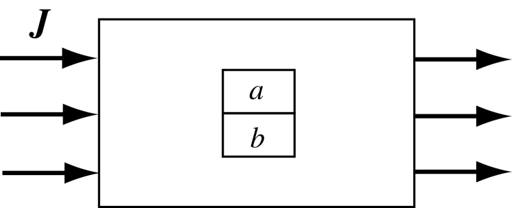
Figure 1: The total system with a uniform current and its subsystems.

Consider a subsystem $a$ of the total where steady current ${\bf J}$ is present (see Fig. 1). In this subsystem, there is equal amount of energy input and dissipation per unit time, the latter being thrown out of the subsystem by some microscopic degrees of freedom not considered explicitly. Following the philosophy of SST, we disregard this energy flow, include the carrier of the dissipations in “hidden degrees of freedom”Callen , and consider the fluctuations caused by the energy flow and those through the wall of the subsystems together. Now, the system is characterized by the uniform static current ${\bf J}$, whose “energy” may be calculated by the static “Hamiltonian:”

$${\cal H}^{(a)}= \int_{V_{a}}\!\psi^{\dagger}({\bf r})\!\left[\frac{(-i\bm{\nabla}-{\bf p}_{0})^{2}}{2m}+V_{\rm imp}({\bf r})-\mu\right]\!\psi({\bf r})\,d{\bf r}\,,$$

where ${\bf p}_{0}$ is a variable conjugate to ${\bf J}$. From now on we can follow the argument of equilibrium statistical mechanics to derive the density matrix $\rho^{(a)}$ of the subsystem $a$: Since it is time-independent by assumption, $\rho^{(a)}$ commutes with ${\cal H}^{(a)}$, so that it is a function of the eigenvalue ${\cal E}_{\nu}^{(a)}$ of ${\cal H}^{(a)}$. From (ii) the statistical independence, $\rho^{(a+b)}=\rho^{(a)}\rho^{(b)}$, and (iii) additivity of energy, ${\cal E}^{(a+b)}={\cal E}^{(a)}+{\cal E}^{(b)}$, it follows thatLL

$$\ln\rho_{\nu}^{(a)}=\alpha^{(a)}-\beta{\cal E}_{\nu}^{(a)}\,,$$ (6)

where $\alpha^{(a)}$ and $\beta$ are some constants. Normalizing $\rho^{(a)}$, we have

$$\rho^{(a)}_{\nu}=\frac{{\rm e}^{-\beta{\cal E}_{\nu}^{(a)}}}{\displaystyle\sum_{\mu}{\rm e}^{-\beta{\cal E}_{\mu}^{(a)}}}\,,$$ (7)

where higher probability for lower ${\cal E}$ means $\beta>0$. Thus, we have reached a candidate for the steady state density matrix in the presence of a uniform current $\bf J$.

We now see that Eq. (7) corresponds to the state of maximum entropy, following exactly the argument of equilibrium caseLL : Entropy is defined by $S^{(a)}\equiv-{\rm Tr}\rho^{(a)}\ln\rho^{(a)}\equiv-\left<\ln\rho^{(a)}\right>$ and calculated by using Eqs. (LABEL:H2) and (6) as

$$S^{(a)} =-\alpha^{(a)}+\beta\langle{\cal E}^{(a)}\rangle$$ (8)

$$=-\alpha^{(a)}+\beta(\langle E^{(a)}\rangle-\mu^{\prime}\langle N^{(a)}\rangle-{\bf p}_{0}\cdot\langle{\bf J}^{(a)}\rangle)\,,$$

where $E^{(a)}$ is the energy of the subsystem, $\langle{\bf J}^{(a)}\rangle\equiv-\langle\partial{\cal H}^{(a)}/\partial{\bf p}_{0}\rangle$, and $\mu^{\prime}\equiv\mu+\frac{p_{0}^{2}}{2m}$. We also notice that $-\langle\ln\rho^{(a)}\rangle=-\ln\rho^{(a)}(\langle{\cal E}\rangle)$. On the other hand, Eq. (7) tells us that the probability is the same for all degenerate states and equal in the thermodynamic limit to the inverse of the number of states around $\langle{\cal E}^{(a)}\rangle$. Hence Eq. (8) corresponds to the entropy maximum for the energy $\langle E^{(a)}\rangle$, the electron number $\langle N^{(a)}\rangle$, and the current $\langle{\bf J}^{(a)}\rangle$. Finally, we may perform the Legendre transformation $G^{(a)}\equiv\langle{\cal H}^{(a)}\rangle+{\bf p}_{0}\cdot\langle{\bf J}^{(a)}\rangle$ to obtain the desired free energy $G^{(a)}$ as a function of $\beta$, $\mu^{\prime}$, and $\langle{\bf J}^{(a)}\rangle$.

The above consideration can be applied to any uniform steady states driven by mechanical forces. Indeed, we only have to introduce in the Hamiltonian a variable [such as ${\bf p}_{0}$ in Eq. (LABEL:H2)] which is conjugate to the expectation value (such as ${\bf J}$ in the above consideration) characterizing the steady state.

Several comments are in order. First, the consideration here puts aside completely the driving force ${\bf E}$ and the corresponding dissipations. Thus, this density matrix cannot say anything about the ${\bf E}$-${\bf J}$ relation, but only identifies the steady state for a given ${\bf J}$. However, this ${\bf E}$-${\bf J}$ relation may be obtained by connecting the results through the linear-response calculations for each ${\bf J}$. Second, the above argument starts from three plausible basic assumptions on uniform steady states: (i) equivalence between any two subsystems of the total, (ii) statistical independence between any two subsystems, and (iii) additivity of energy. Hence we may expect that the derived Gibbs distribution (7) is the correct distribution for those steady states. Indeed, there are several stochastic models which realize the Gibbs distribution in nonequilibrium steady states.OY87 ; Takesue87 ; Yeung89 However, it should be noted that the quantity $\beta$ here includes the fluctuation of energy due to dissipations as well as that through the walls among subsystems. If the former contribution is negligible, we may expect that $\beta$ is the same as the equilibrium value. Experimentally, there remains a basic problem on how to measure the value of $\beta$ for the steady states. Third, the above consideration have surely made the concept of “state space” in SST clearer. The postulated second-law of SST may be proved now by using Eq. (7) and the Jarzynski identityJarzynski . Fourth, the subsystem considered here may contain structures small compared with the subsystem size such as the vortex lattice structures.

There are many interesting nonequilibrium phenomena found in semiconductors.Scholl Also, Stoll et al. found steps in the $I$-$V$ characteristics in the vortex state of superconducting Nd_2-xCe_xCuO_y; this first-order-like transition may be described by the nonequilibrium free energy derived above, as increasing ${\bf E}$ causes the density-of-states (DOS) change in the electron system.

I am grateful for Koji Nemoto for an enlightening discussion.

References

- (1) S. R. de Groot and P. Mazur, Non-Equilibrium Thermodynamics (North-Holland, Amsterdam, 1962).
- (2) D. D. Fitts, Nonequilibrium Thermodynamics: a Phenomenological Theory of Irreversible Processes in Fluid Systems (McGraw-Hill, New York, 1962).
- (3) P. Glansdorff and I. Prigogine, Thermodynamic Theory of Structure, Stability and Fluctuations (Wiley-Interscience, London, 1971).
- (4) D. N. Zubarev, Nonequilibrium Statistical Thermodynamics (Consultants Bureau, New York, 1974).
- (5) R. Landauer, Phys. Rev. A18, 255 (1978); Physica A194, 551 (1993).
- (6) J. Keizer, Statistical Thermodynamics of Nonequilibrium Processes (Springer-Verlag, Berlin, 1987).
- (7) D. Jou, J. Casas-Vázques, and G. Lebon, Extended Irreversible Thermodynamics (Springer-Verlag, Berlin, 1993).
- (8) G. L. Eyink, J. L. Lebowitz, and H. Spohn, J. Stat. Phys. 83, 385 (1996).
- (9) Y. Oono and M. Paniconi, Prog. Theor. Phys. Suppl. 130, 29 (1998).
- (10) L. Onsager, Phys. Rev. 37, 405 (1931); 38, 2265 (1931).
- (11) H. B. Callen, Thermodynamics (John Wiley, New York, 1960).
- (12) K. Sekimoto, Prog. Theor. Phys. Suppl. 130, 17 (1998).
- (13) T. Hatano, Phys. Rev. E 60, R5017 (1999).
- (14) T. Hatano and S. Sasa, Phys. Rev. Lett. 86, 3463 (2001).
- (15) T. Shibata, cond-mat/0012404.
- (16) S. Sasa and H. Tasaki, cond-mat/00108365.
- (17) R. Kubo, M. Toda, and N. Hashitsume, Nonequilibrium statistical mechanics (Springer-Verlag, Berlin, 1991).
- (18) L. V. Keldysh, Zh. Eksp. Teor. Fiz. 47, 1515 (1964) [Sov. Phys. JETP 20, 1018 (1965).
- (19) For a review, see for example, J. Rammer and H. Smith, Rev. Mod. Phys. 58, 323 (1986); H. Haug and A.-P. Jauho, Quantum Kinetics in Transport and Optics of Semiconductors (Springer, Berlin, 1998) Chap 4.
- (20) L. D. Landau and E. M. Lifshitz, Statistical Physics (Pergamon, Oxford, 1980) §7.
- (21) Y. Oono and C. Yeung, J. Stat. Phys. 48, 593 (1987).
- (22) S. Takesue, Phys. Rev. Lett. 59, 2499 (1987).
- (23) C. Yeung, J. Stat. Phys. 55, 357 (1989).
- (24) C. Jarzynski, Phys. Rev. Lett. 78, 2690 (1997).
- (25) E. Schöll, Nonequilibrium Phase Transitions in Semiconductors (Springer-Verlag, Berlin, 1987)
- (26) O. M. Stroll, R. P. Hübener, S. Kaiser, and M. Naito, Phys. Rev. B60, 12424 (1999).