[

Enhanced mesoscopic fluctuations in the crossover between random matrix ensembles

Abstract

In random-matrix ensembles that interpolate between the three basic ensembles (orthogonal, unitary, and symplectic), there exist correlations between elements of the same eigenvector and between different eigenvectors. We study such correlations, using a remarkable correspondence between the interpolating ensembles late in the crossover and a basic ensemble of finite size. In small metal grains or semiconductor quantum dots, the correlations between different eigenvectors lead to enhanced fluctuations of the electron-electron interaction matrix elements which become parametrically larger than the non-universal fluctuations.

]

Random matrix theory has focused on the study of three ensembles of Hamiltonians: the Gaussian Unitary Ensemble (GUE), the Gaussian Orthogonal Ensemble (GOE), and the Gaussian Symplectic Ensemble (GSE). These describe the statistics of single-particle energy levels and wavefunctions of disordered metal grains or chaotic quantum dots with the corresponding symmetries; GUE if time-reversal symmetry is broken, and GOE or GSE if time-reversal symmetry is present and spin-rotation symmetry is present or absent, respectively. In these three basic ensembles, eigenvector elements are Gaussian complex/real/quaternion random numbers; elements of the same eigenvector and of different eigenvectors are all statistically independent [2].

Disordered or chaotic systems with partially broken symmetries show a variety of phenomena that go beyond a mere “interpolation” of descriptions based on the GOE, GUE, and GSE alone. For example, in a quantum dot, a weak magnetic field causes long-range wavefunction correlations [3, 4, 5] and a non-Gaussian distribution of “level velocities”, derivatives of energy levels with respect to, e.g., a shape change of the dot [6]. Both effects are absent without a magnetic field (in the GOE), or when the magnetic field is strong enough to fully break time-reversal symmetry (in the GUE). In a metal grain, weak spin-orbit interaction induces mesoscopic fluctuations of the $g$-tensor [7, 8], which does not fluctuate in either the GOE or the GSE. Further, as we’ll show below, in a weak magnetic field or for weak spin-orbit scattering, matrix elements of the electron-electron interaction exhibit fluctuations that are parametrically larger than in each of the three basic ensembles.

The underlying reason for these phenomena is that eigenvector elements are not independent in (random-matrix) ensembles that interpolate between the three basic symmetry classes: There exist both correlations within the same eigenvector [3, 4, 5, 6, 7] and, as we show in this letter, between different eigenvectors. To study the eigenvector correlations in such crossover ensembles, we will make use of a surprising relation between the eigenvector statistics late in the crossover from class A to class B and that of finite-sized matrices in class B (where B is the class of lower symmetry). Examples of such a relation were known for the statistics of a single eigenvector. For example, in the GOE-GUE crossover, which is described by the $N\times N$ random hermitian matrix (with $N$ taken to $\infty$ at the end of the calculation) [9]

$$H_{\rm OU}(N,\alpha)=H_{\rm O}(N)+{\alpha\over\sqrt{N}}H_{\rm U}(N),$$ (1)

the distribution of the “phase rigidity” $|{\mbox{\boldmath$v$}}^{\rm T}{\mbox{\boldmath$v$}}|^{2}$ [6] of a single eigenvector $v$ is the same as in the finite-sized $M\times M$ GUE ensemble with $M=2\alpha^{2}$ if $\alpha$ is large. In Eq. (1), $H_{\rm O}(N)$ and $H_{\rm U}(N)$ are $N\times N$ matrices taken from the GOE and GUE, respectively, with equal variances for the matrix elements. A similar correspondence occurs for the $g$-tensor of a Kramers doublet in the GOE-GSE crossover [7, 8]. Our main finding is that such a correspondence extends to the correlations between different eigenvectors.

In this paper we will accomplish four tasks. (i) We show numerically that the relation

$$H_{\rm OU}(N,\alpha)\leftrightarrow H_{\rm U}(M),\ \ M=2\alpha^{2}$$ (2)

between the GOE-GUE crossover Hamiltonian $H_{\rm OU}(\alpha)$ for large $\alpha$ and $N$ and a finite-sized $M\times M$ GUE Hamiltonian extends to correlations between eigenvectors. Just as in critical phenomena, where simple power laws unfold into universal scaling functions as you flow away from the critical point, here a rich theory of correlations unfolds in the crossover region. We wish to point out that this principle applies not only to the GOE-GUE crossover, but also, e.g., to the GOE-GSE crossover, or to wavefunctions in two coupled quantum dots, which are described by a random Hamiltonian interpolating between two independent GUE’s and one GUE of double size [10]. (ii) We show that, for large $\alpha$, the universality classes are actually curves in the $(1/\alpha,1/N)$ plane, reminiscent of renormalization-group flow trajectories [11]. (iii) We calculate correlations between eigenvectors, based on the surmise (2) and diagrammatic perturbation theory. (iv) We calculate how the inter-eigenvector correlations in the crossover region affect matrix elements of the electron-electron interaction in a quantum dot or metal grain in a weak magnetic field, and predict a significant enhancement of fluctuations compared to the basic ensembles.

Let us now consider the joint distribution $P(\{\mbox{\boldmath$v$}_{\mu}\})$ of $n$ eigenvectors ${\mbox{\boldmath$v$}}_{\mu}$, $\mu=1,\ldots,n$, for the example of the GOE-GUE crossover Hamiltonian (1). Throughout the entire GOE-GUE crossover, the distribution of the eigenvectors is invariant under orthogonal transformations. As a consequence, the joint distribution $P(\{{\mbox{\boldmath$v$}}_{\mu}\})$ is completely determined by the distribution of the orthogonal invariants [3, 4]

$$\rho_{\mu\nu}=\rho_{\nu\mu}={\mbox{\boldmath$v$}}^{\rm T}_{\mu}{\mbox{\boldmath$v$}}^{\vphantom{T}}_{\nu},\ \ \mu,\nu=1,\ldots,n,$$ (3)

where the superscript ${\rm T}$ denotes transposition. Hence

$$P(\{{\mbox{\boldmath$v$}}_{\mu}\}) = \int\prod_{\mu\leq\nu}^{n}d\rho_{\mu\nu}\,P(\{\rho_{\mu\nu}\})$$ (5)

$$\mbox{}\times\prod_{\mu\leq\nu}^{n}\delta({\mbox{\boldmath$v$}}_{\mu}^{\dagger}{\mbox{\boldmath$v$}}_{\nu}-\delta_{\mu\nu})\delta({\mbox{\boldmath$v$}}_{\mu}^{\rm T}{\mbox{\boldmath$v$}}_{\nu}-\rho_{\mu\nu}).$$

For the physically relevant case of large $N$, Eq. (5) implies that the eigenvector elements ${\mbox{\boldmath$v$}}_{\mu m}$, $m=1,\ldots,N$, have a Gaussian distribution with zero mean and

$$\langle v_{\mu m}^{*}v_{\nu n}\rangle_{\rho}=N^{-1}\delta_{\mu\nu}\delta_{mn},\ \ \langle v_{\mu m}v_{\nu n}\rangle_{\rho}=\rho_{\mu\nu}\delta_{mn}.$$ (6)

The subscript $\langle\ldots\rangle_{\rho}$ indicates that the average is taken at fixed $\rho_{\mu\nu}$. For the full ensemble average one has to perform a subsequent average over the $\rho_{\mu\nu}$ with the distribution $P(\{\rho_{\mu\nu}\})$. We can find $P(\{\rho_{\mu\nu}\})$ from the surmise that, for $\alpha\gg 1$ and for eigenvectors ${\mbox{\boldmath$v$}}_{\mu}$ whose energies are all inside a window of size $\lesssim\alpha^{2}\Delta$, $\Delta$ being the level spacing of the Hamiltonian $H(\alpha)$, the joint distribution of the $\rho_{\mu\nu}$ is the same as for a GUE Hamiltonian of finite size $M=2\alpha^{2}$. Thus the $\rho_{\mu\nu}$ are independently and Gaussian distributed with zero mean and with variance

$$\langle|\rho_{\mu\nu}|^{2}\rangle=(1+\delta_{\mu\nu})/M,\ \ M=2\alpha^{2}.$$ (7)

Together, Eqs. (5)–(7) fix the joint distribution of eigenvectors in the crossover ensemble close to the GUE. For the single-eigenvector distribution, Eqs. (5)–(7) reproduce the $\alpha\gg 1$ limit of the exact solution of Sommers and Iida [4]. The fact that the phase rigidity $|\rho_{\mu\mu}|^{2}$ of a single eigenvector is a fluctuating quantity is the prime cause of the correlations between elements of one eigenvector [5, 6]; It is the existence of nonzero and fluctuating $\rho_{\mu\nu}$ for $\mu\neq\nu$ that causes the correlations between different eigenvectors.

We now proceed to present arguments in support of our surmise. We consider the eigenvectors ${\mbox{\boldmath$v$}}_{\mu}$ ($\mu=1,\ldots,n$) with energies within a distance $\ll\alpha^{2}\Delta$ from a reference energy $\varepsilon_{\rm ref}$, sorting them by increasing energy. We then consider how each of these eigenvectors is built up from the eigenvectors ${\mbox{\boldmath$o$}}_{\nu}$ of the unperturbed Hamiltonian $H_{\rm O}$. Contributions from eigenvectors ${\mbox{\boldmath$o$}}_{\nu}$ with energy $\varepsilon_{\nu}$ far away from $\varepsilon_{\rm ref}$ can be described using perturbation theory in the crossover parameter $\alpha$. If the energy difference $\varepsilon_{\rm ref}-\varepsilon_{\nu}$ is sufficiently large, the admixture of ${\mbox{\boldmath$o$}}_{\nu}$ to any of the vectors ${\mbox{\boldmath$v$}}_{\mu}(\alpha)$ of interest is small and can be neglected. On the other hand, eigenvectors ${\mbox{\boldmath$o$}}_{\nu}$ with energy $\varepsilon_{\nu}$ close to $\varepsilon_{\rm ref}$ contribute non-perturbatively for large $\alpha$. Upon increasing $\alpha$ from zero, the eigenvectors ${\mbox{\boldmath$v$}}_{\mu}(\alpha)$ in this energy range have undergone several avoided crossings, and the unperturbed eigenvectors ${\mbox{\boldmath$o$}}_{\mu}$ have roughly equal weights in each of the vectors ${\mbox{\boldmath$v$}}_{\mu}(\alpha)$ in our set.

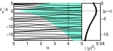
FIG. 1.: Left panel: Eigenvalues for one realization of $H_{\rm OU}(\alpha)$. The shaded region marks the energy window of size $\sim M(\alpha)\Delta=2\alpha^{2}\Delta$ for which the eigenvalues are kept in the effective $M\times M$ GUE Hamiltonian. Right panel: $\langle|\rho_{\mu\nu}|^{2}\rangle$ as a function of the distance $\mu-\nu\approx(\varepsilon_{\mu}-\varepsilon_{\nu})/\Delta$ between eigenvalues, for $\alpha=4.0$ (dashed line, left panel). Solid curve: Eq. (11). Data points: numerical calculation for $N=400$.

It is on this heuristic picture that our surmise for an effective description of the eigenvector statistics for large $\alpha$ is based: We only retain those eigenvectors of the unperturbed Hamiltonian $H_{\rm O}$ that are relatively close in energy and hence all contribute roughly equally, see Fig. 1 for a cartoon. Since the time-reversal symmetry breaking perturbation in Eq. (1) is strong for these eigenvectors, the matrix elements between them form a random hermitian matrix of the GUE. Denoting the effective number of contributing unperturbed eigenvectors as $M(\alpha)$, we thus reduce the problem of finding the distribution of the orthogonal invariants $\rho_{\mu\nu}$ for the $N\times N$ crossover Hamiltonian (1) to that of finding the distribution of the $\rho_{\mu\nu}$ for the much smaller GUE Hamiltonian of size $M(\alpha)$. To calculate $M(\alpha)$ in terms of $N$ and $\alpha$, we turn to the exact solution for the single-eigenvector distribution obtained in Refs. [4, 5, 6], and find [12]

$$M(\alpha)=\alpha^{2}N(\alpha^{2}+2N)/(\alpha^{2}+N)^{2}.$$ (8)

For large $N$ this simplifies to $M(\alpha)=2\alpha^{2}$, in agreement with Eq. (7).

By our surmise, the distribution of the orthogonal invariants should depend on the effective matrix size $M(\alpha)$ only, not on $\alpha$ and $N$ individually, as long as $N$ and $\alpha$ are large. We have verified this by numerical calculation of the averages $\langle|\rho_{\mu\nu}|^{2}\rangle$ for different points along a curve of constant $M(\alpha)$ in the $(1/N,1/\alpha)$ plane. The results of such a calculation are shown in Fig. 2 for $\mu=\nu$, for neighboring eigenvectors ($\mu=\nu+1$) and for next-nearest neighbors ($\mu=\nu+2$). We have also verified that the distribution of the $\rho_{\mu\nu}$ is indeed Gaussian (not shown).

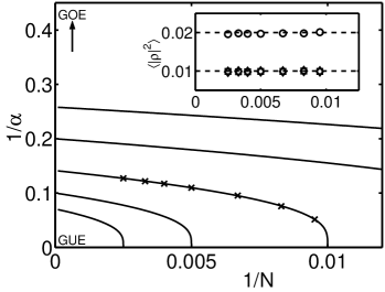
FIG. 2.: Curves of constant effective GUE size $M(\alpha)$, Eq. (8), in the $(1/\alpha,1/N)$ plane for the $N\times N$ crossover Hamiltonian (1). Top to bottom: $M=20$, $M=30$, $M=50$, $M=100$, and $M=200$. The horizontal and vertical axes correspond to the pure GUE and to the $N\to\infty$ crossover Hamiltonian, respectively. Inset: $\langle|\rho_{\mu\nu}|^{2}\rangle$ for the points indicated at the $M=50$ curve in the main panel. Circles: $\mu=\nu$; Squares: $\mu=\nu+1$ (eigenvectors with neighboring energy levels); diamonds: $\mu=\nu+2$ (next-nearest neighbors). The dashed lines indicate the surmise of Eq. (7).

The surmise (2) is expected to be valid as long as only eigenvectors taken from an energy window of width $\ll M(\alpha)\Delta=2\alpha^{2}\Delta$ are involved. If the energy differences between eigenvectors become of order $\alpha^{2}\Delta$ or larger, the eigenvectors ${\mbox{\boldmath$v$}}_{\mu}(\alpha)$ do not share the same unperturbed eigenvectors ${\mbox{\boldmath$o$}}_{\nu}$, and we thus expect that they become uncorrelated. A quantitative description of eigenvector correlations at energy separations $\gg\Delta$ can be obtained using diagrammatic perturbation theory. The only nonzero second moment is $\langle|\rho_{\mu\nu}|^{2}\rangle$, which can be computed from

$$\langle|\rho_{\mu\nu}|^{2}\rangle = -{\Delta^{2}\over 4\pi^{2}}\sum_{s_{1},s_{2}=\pm}s_{1}s_{2}$$ (10)

$$\mbox{}\times\left\langle\mbox{tr}\,G^{\rm T}(\varepsilon_{\mu}+is_{1}\delta)G(\varepsilon_{\nu}+is_{2}\delta)\right\rangle.$$

where $G(z)=1/(z-H_{\rm OU})$, $\delta$ is a positive infinitesimal, and the eigenvectors ${\mbox{\boldmath$v$}}_{\mu}$ and ${\mbox{\boldmath$v$}}_{\nu}$ have energies $\varepsilon_{\mu}$ and $\varepsilon_{\nu}$, respectively. Calculating the averages using the technique of Ref. [13], we find, if $\mu\neq\nu$,

$$\langle|\rho_{\mu\nu}|^{2}\rangle={2\alpha^{2}\over 4\alpha^{4}+\pi^{2}(\varepsilon_{\mu}-\varepsilon_{\nu})^{2}/\Delta^{2}}.$$ (11)

A similar result for parametric correlations inside a basic random-matrix ensemble was derived in Ref. [14]. The right panel of Fig. 1 shows $\langle|\rho_{\mu\nu}|^{2}\rangle$ as a function of $\varepsilon_{\mu}-\varepsilon_{\nu}$ and a numerical calculation of the same quantity.

The GOE-GUE crossover that we considered here describes the wavefunction statistics in, e.g., a chaotic quantum dot or a disordered metal grain in a weak magnetic field. Wavefunction distributions have immediate experimental relevance for the spacings, widths, and heights of Coulomb blockade peaks in the conductance of metal grains or quantum dots [15]. Correlations between wavefunctions of neighboring energy levels cause correlations between the heights and widths of neighboring conductance peaks. Wavefunction distributions also influence the positions of Coulomb blockade peaks through their role in the distribution of electron-electron interaction matrix elements [16], which we now discuss in detail. The interaction matrix element $U_{\mu\nu\rho\sigma}$ is defined as

$$U_{\mu\nu\rho\sigma} = \int d\vec{r}_{1}d\vec{r}_{2}U(\vec{r}_{1}-\vec{r}_{2})$$ (13)

$$\mbox{}\times\phi_{\mu}(\vec{r}_{1})\phi_{\nu}(\vec{r}_{2})\phi_{\rho}(\vec{r}_{2})^{*}\phi_{\sigma}(\vec{r}_{1})^{*},$$

where $U(\vec{r})$ is the electron-electron interaction potential and $\phi_{\mu}(\vec{r})$ the wavefunction for an electron in level $\varepsilon_{\mu}$. For example, the difference of interaction matrix elements $U_{\mu\mu\nu\nu}-U_{\mu\mu oo}$ gives the spacing between peak positions corresponding to different nonequilibrium configurations (levels $\nu$ and $o$ unoccupied, respectively) in tunneling spectroscopy of small metal grains [17].

In a metal grain or quantum dot, the interaction can be approximated by an $\vec{r}$-independent part and a local interaction $U^{\rm loc}(\vec{r})=\lambda\Delta V\delta(\vec{r})$, where $\Delta$ is the mean level spacing, $V$ is the sample volume, and $\lambda$ is a parameter of order unity governing the strength of the local interaction. The spatially constant interaction leads to a charging energy and does not show mesoscopic fluctuations. For the GOE (no magnetic field), the matrix elements of $U^{\rm loc}$ have an average given by [15]

$$\langle U^{\rm loc}_{\mu\nu\rho\sigma}\rangle=\lambda\Delta(\delta_{\mu\sigma}\delta_{\nu\rho}+\delta_{\mu\rho}\delta_{\nu\sigma}+\delta_{\mu\nu}\delta_{\rho\sigma}).$$ (14)

If time-reversal symmetry is broken by a magnetic field (i.e., in the GUE), the last term in Eq. (14) is left out [18]. In both the GOE and GUE, fluctuations of the interaction matrix elements $U^{\rm loc}_{\mu\nu\rho\sigma}$ and corrections to Eq. (14) are nonuniversal and small as (at most) $g^{-1/2}$, where $g$ is the dimensionless conductance of the sample. Equation (14) can be reproduced from random-matrix theory if the wavefunctions $\phi_{\mu}(\vec{r})$ are replaced by eigenvectors ${\mbox{\boldmath$v$}}_{\mu}$ and the integration over space is replaced by a summation over the vector indices.

How are the interaction matrix elements distributed in the presence of a weak magnetic field? If we are not interested in the non-universal ($1/g$) corrections, that question can be answered using the eigenvector distributions for the GOE-GUE crossover that we derived above. First, upon increasing the magnetic field, there is a gradual suppression of the last term in Eq. (14). However, as a result of gauge invariance (wave-functions can be multiplied with an arbitrary phase factor), the average of the last term in Eq. (14) is formally zero throughout the crossover if $\mu\neq\rho$, and this effect only shows up in the fluctuations of $U_{\mu\nu\rho\sigma}$. Second, the appearance of inter-eigenvector correlations enhances the average of all interaction matrix elements. Using Eq. (6), we find

$$\langle U_{\mu\nu\rho\sigma}^{\rm loc}\rangle = \lambda\Delta(\delta_{\mu\rho}\delta_{\nu\sigma}+\delta_{\mu\sigma}\delta_{\nu\rho}+\langle\rho_{\mu\nu}\rho_{\rho\sigma}\rangle).$$ (15)

For large $\alpha$, the average $\langle\rho_{\mu\nu}\rho_{\rho\sigma}\rangle$ can be done with the help of Eqs. (7) and (11), with the result

$$\langle U_{\mu\nu\rho\sigma}^{\rm loc}\rangle = \lambda\Delta(\delta_{\mu\rho}\delta_{\nu\sigma}+\delta_{\mu\sigma}\delta_{\nu\rho})$$ (17)

$$\mbox{}\times\left(1+{2\alpha^{2}\over 4\alpha^{4}+\pi^{2}(\varepsilon_{\mu}-\varepsilon_{\nu})^{2}/\Delta^{2}}\right).$$

Third, the inter-eigenvector correlations enhance the fluctuations of the interaction matrix elements. This is best illustrated by the expectation value $\langle|U_{\mu\nu\rho\sigma}|^{2}\rangle$ with all four indices $\mu$, $\nu$, $\rho$, and $\sigma$ different,

$$\langle|U_{\mu\nu\rho\sigma}^{\rm loc}|^{2}\rangle = (\lambda\Delta)^{2}\langle|\rho_{\mu\nu}|^{2}|\rho_{\rho\sigma}|^{2}\rangle=(\lambda\Delta)^{2}/(2\alpha^{2})^{2}.$$ (18)

The first equality in Eq. (18) holds for all $\alpha$, the second one only if $\alpha\gg 1$ and the four eigenvalues $\varepsilon_{\mu}$, $\varepsilon_{\nu}$, $\varepsilon_{\rho}$, $\varepsilon_{\sigma}$ are within a distance $\ll\alpha^{2}\Delta$ of each other. We have numerically calculated $\langle|U_{\mu\nu\rho\sigma}^{\rm loc}|^{2}\rangle$ for four neighboring wavefunctions as a function of $\alpha$ throughout the entire GOE-GUE crossover, see Fig. 3.

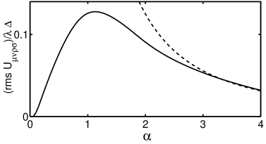
FIG. 3.: Root-mean-square fluctuations of the interaction matrix element $U_{\mu\nu\rho\sigma}$ for four consecutive levels $\mu=\nu-1$ $=\rho-2=\sigma-3$. The dashed line shows the large-$\alpha$ asymptote of Eq. (18). The solid line is obtained from numerical generation of $400\times 400$ GOE-GUE crossover matrices, using $\langle|U_{\rm\mu\nu\rho\sigma}|^{2}\rangle=(\lambda\Delta)^{2}\langle|\rho_{\mu\nu}|^{2}|\rho_{\rho\sigma}|^{2}\rangle$. (Direct numerical calculation of $U_{\rm\mu\nu\rho\sigma}$ suffers from large finite-$N$ corrections.)

Note that the enhanced fluctuations appear in matrix elements that are not commonly associated with the presence of time-reversal symmetry. Although the fluctuations are small if $\alpha\gg 1$, they can be significantly larger than the non-universal fluctuations that vanish as $g^{-2}$ [for Eq. (18)]. These extra large fluctuations can be an additional source of fluctuations of Coulomb-blockade peak positions, and may dominate over the non-universal sources of fluctuations.

The origin of the eigenvector correlations and the enhanced fluctuations of interaction matrix elements can be sought in the existence of the large parameter $\alpha^{2}$ that plays a role similar to the dimensionless conductance $g$ in the pure ensembles. The parameter $\alpha^{2}$ can be identified as the ratio of the Heisenberg time $\tau_{\rm H}=2\pi\hbar/\Delta$ and the time $\tau_{\rm OU}$ needed to acquire a flux quantum [15]. Late in the crossover, GUE physics ranges from the mean level spacing $\Delta$ up to the scale $\hbar/\tau_{\rm OU}$. In the pure GUE, however, validity of random-matrix theory ceases only at the higher energy scale $\hbar/\tau_{\rm erg}$, where $\tau_{\rm erg}$ is the ergodic time. The role of the large parameter $g=\tau_{\rm H}/\tau_{\rm erg}$, which governs wavefunction correlations and interaction matrix element fluctuations in the “pure” GUE and GOE is thus played by $\alpha^{2}\sim\tau_{\rm H}/\tau_{\rm OH}$ in the GOE-GUE crossover.

We thank Yuval Oreg and Dan Ralph for discussions. This work was supported in part by the NSF under grants no. DMR 0086509 and KDI 9873214 and by the Sloan and Packard foundations.

REFERENCES

- [1] Present address: CEA, Service de Physique de l’Etat Condensé, Centre d’Etudes de Saclay, 91191 Gif-sur-Yvette, France.
- [2] M. L. Mehta, Random Matrices (Academic, New York, 1991).
- [3] J. B. French, V. K. B. Kota, A. Pandey, and S. Tomsovic, Ann. Phys. (N. Y.) 181, 198 (1988).
- [4] H.-J. Sommers and S. Iida, Phys. Rev. E 49, 2513 (1994).
- [5] V. I. Fal’ko and K. B. Efetov, Phys. Rev. B 50, 11267 (1994); Phys. Rev. Lett. 77, 912 (1996).
- [6] S. A. van Langen, P. W. Brouwer, and C. W. J. Beenakker, Phys. Rev. E 55, 1 (1997).
- [7] P. W. Brouwer, X. Waintal, and B. I. Halperin, Phys. Rev. Lett. 85, 369 (2000).
- [8] K. A. Matveev, L. I. Glazman, and A. I. Larkin, Phys. Rev. Lett. 85, 2789 (2000).
- [9] A. Pandey and M. L. Mehta, Commun. Math. Phys. 87, 449 (1983).
- [10] Single-eigenvector statistics for this case are studied in A. Tschersich and K. B. Efetov, Phys. Rev. E 62, 2042 (2000).
- [11] Renormalization group ideas have been applied previously to study universality and deviations from universality in the three basic ensembles of random matrix theory. See, e.g., E. Brézin and J. Zinn-Justin, Phys. Lett. B 288, 54 (1992); E Brézin and A. Zee, Compt. Rend. Acad. Sci 17, 735 (1993); S. Higuchi, C. Itoi, S. Hishigaki, and N. Sakai, Nucl. Phys. B 434, 283 (1995).
- [12] A rough estimate of can be obtained by comparing the contributions to from unperturbed eigenvectors with energy close to (far away) from , which are (are not) included in the effective GUE Hamiltonian. In the former case, the weight of is , whereas in the latter case it is , where is the mean square of an element of . Comparing the two estimates at the energy difference separating the two regimes, we conclude , in agreement with the exact result (8).
- [13] E. Brézin and A. Zee, Phys. Rev. E 49, 2588 (1994).
- [14] M. Wilkinson and P. N. Walker, J. Phys. A 28, 6143 (1995).
- [15] I. L. Aleiner, P. W. Brouwer, and L. I. Glazman, Phys. Rep., Phys. Rep. 358, 309 (2002).
- [16] J. von Delft and D. C. Ralph, Phys. Rep. 345, 61 (2001).
- [17] O. Agam, N. S. Wingreen, B. L. Altshuler, D. C. Ralph, and M. Tinkham, Phys. Rev. Lett. 78, 1956 (1997).
- [18] The last term in Eq. (14) also vanishes in the GOE once the renormalization of the local interaction from virtual excitations is taken into account, see, e.g., Ref. [15].