Pairing fluctuation theory of high $T_{c}$ superconductivity in the presence of nonmagnetic impurities

Abstract

The pseudogap phenomena in the cuprate superconductors requires a theory beyond the mean field BCS level. A natural candidate is to include strong pairing fluctuations, and treat the two-particle and single particle Green’s functions self-consistently. At the same time, impurities are present in even the cleanest samples of the cuprates. Some impurity effects can help reveal whether the pseudogap has a superconducting origin and thus test various theories. Here we extend the pairing fluctuation theory for a clean system [Phys. Rev. Lett. 81, 4708 (1998)] to the case with nonmagnetic impurities. Both the pairing and the impurity $T$ matrices are included and treated self-consistently. We obtain a set of three equations for the chemical potential $\mu$, $T_{c}$, the excitation gap $\Delta(T_{c})$ at $T_{c}$, or $\mu$, the order parameter $\Delta_{sc}$, and the pseudogap $\Delta_{pg}$ at temperature $T<T_{c}$, and study the effects of impurity scattering on the density of states, $T_{c}$ and the order parameter, and the pseudogap. Both $T_{c}$ and the order parameter as well as the total excitation gap are suppressed, whereas the pseudogap is not for given $T\leq T_{c}$. Born scatterers are about twice as effective as unitary scatterers in suppressing $T_{c}$ and the gap. In the strong pseudogap regime, pair excitations contribute a new $T^{3/2}$ term to the low $T$ superfluid density. The initial rapid drop of the zero $T$ superfluid density in the unitary limit as a function of impurity concentration $n_{i}$ also agrees with experiment.

I Introduction

The pseudogap phenomena in high $T_{c}$ superconductors have been a great challenge to condensed matter physicists since over a decade ago. These phenomena manifestly contradict BCS theory by, e.g, presenting a pseudo excitation gap in single particle excitation spectrum. Yet the origin of the pseudogap and, in general, the mechanism of the superconductivity are still not clear. Many theories have been proposed, which fall into two classes, based on whether the pseudogap has a superconducting origin. Some authors propose that the pseudogap may not be related to the superconductivity; instead, it is associated with another ordered state, such as the antiferromagnetism related resonating valence bond (RVB) state,Anderson (1987) d-density waveChakravarty et al. (2001) and spin density wave order.Demler et al. (2001) On the other hand, many others believe that the pseudogap has the same origin as the superconductivity, such as the phase fluctuation scenario of Emery and KivelsonEmery and Kivelson (1995) and the various precursor superconductivity scenarios.Randeria (1995); Maly et al. (1999a, b); Janko et al. (1997); Chen et al. (1998); Kosztin et al. (1998) Previously, Chen and coworkers have worked out, within the precursor conductivity school, a pairing fluctuation theoryChen et al. (1998, 1999, 2000a) which enables one to calculate quantitatively physical quantities such as the phase diagram, the superfluid density, etc. for a clean system. In this theory, two-particle and one-particle Green’s functions are treated on an equal footing, and equations are solved self-consistently. Finite center-of-mass momentum pair excitations become important as the pairing interaction becomes strong, and lead to a pseudogap in the excitation spectrum. In this context, these authors have been able to obtain a phase diagram and calculate the superfluid density, in (semi)quantitative agreement with experiment.

However, to fully apply this theory to the cuprates, we need to extend it to impurity cases, since impurities are present even in the cleanest samples of the high $T_{c}$ materials, such as the optimally doped YBa₂Cu₃O_7-δ (YBCO) single crystals. In addition, this is necessary in order to understand the finite frequency conductivity issue. Furthermore, study of how various physical quantities respond to impurity scattering may help to reveal the underlying mechanism of the superconductivity. For example, it can be used to determine whether the pseudogap has a superconducting origin.Kruis et al. (2001) Particularly, it is important to address how $T_{c}$ and the pseudogap itself vary with impurity scattering, especially in the underdoped regime. To this end, one needs to go beyond BCS theory and include the pseudogap as an intrinsic part of the theory. Due to the complexity and technical difficulties of this problem, there has been virtually no work in the field on this important problem.

Among all physical quantities, the density of states (DOS) $N(\omega)$ close to the Fermi level ($\omega=0$) is probably most sensitive to the impurities. Yet different authors have yielded contradictory results in this regard. BCS-based impurity $T$ matrix calculations predict a finite DOS at $\omega=0$,Hirschfeld and Vollhardt (1986); Hirschfeld et al. (1988) which has been used to explain the crossover from $T$ to $T^{2}$ power law for the low temperature superfluid density.Hirschfeld and Goldenfeld (1993) Nonperturbative approaches have also been studied and have yielded different results. Senthil and FisherSenthil and Fisher (1999) find that DOS vanishes according to universal power laws, Pépin and LeePépin and Lee (2001) predict that $N(\omega)$ diverges as $\omega\rightarrow 0$, assuming a strict particle-hole symmetry, and ZieglerZiegler et al. (1998) and coworkers’ calculation shows a rigorous lower bound on $N(\omega)$. Recently, Atkinson et al.Atkinson et al. (2000a) try to resolve these contradictions by fine-tuning the details of the disorders. Nevertheless, all these calculations are based on BCS theory and cannot include the pseudogap in a self-consistent fashion, and thus can only be applied to the low $T$ limit in the underdoped cuprates. Therefore, it is necessary to extend the BCS-based calculations on impurity issues to include the pseudogap self-consistently.

In this paper, we extend the pairing fluctuation theory from clean to impurity cases. Both the impurity scattering and particle-particle scattering $T$ matrices are incorporated and treated self-consistently. This goes far beyond the usual self-consistent (impurity) $T$-matrix calculations at the BCS level by, e.g., Hirschfeld and others.Hirschfeld and Vollhardt (1986); Hirschfeld et al. (1988) In this context, we study the evolution of $T_{c}$ and various gap parameters as a function of the coupling strength, the impurity concentration, the hole doping concentration and the impurity scattering strength. In addition, we study not only the Born and the unitary limits, but also at intermediate scattering strength. We find that the real part of the frequency renormalization can never be set to zero, the chemical potential adjusts itself with the impurity level. As a consequence, the positive and negative strong scattering limits do not meet. The residue density of states at the Fermi level is generally finite at finite impurity concentrations, in agreement with what has been observed experimentally. Both $T_{c}$ and the total excitation gap decrease with increasing impurity level, as one may naively expect. Born scatterers are about twice as effective as unitary scatters in suppressing $T_{c}$ and the gap. In the unitary limit, the zero temperature superfluid density decreases faster with $n_{i}$ when $n_{i}$ is still small, whereas in the Born limit, it is the opposite. At given $T<T_{c}$, both the order parameter and the total gap are suppressed, but the pseudogap is not. Finally, incoherent pair excitations contribute an additional $T^{3/2}$ term to the low $T$ temperature dependence of the superfluid density, robust against impurity scattering.

In the next section, we first review the theory in a clean system, and then present a theory at the Abrikosov-Gor’kov level. Finally, we generalize it to include the full impurity $T$-matrix, in addition to the particle-particle scattering $T$-matrix, in the treatment, and obtain a set of three equations to solve for $\mu$, $T_{c}$ and various gaps. In Sec. III, we present numerical solutions to these equations. We first study the effects of impurity scattering on the density of states, then study the effects on $T_{c}$ and the pseudogap at $T_{c}$, followed by calculations of the effects on the gaps and the superfluid density below $T_{c}$. Finally, we discuss some related issues, and conclude our paper.

II Theoretical Formalism

The excitation gap forms as a consequence of Cooper pairing in BCS theory, while the superconductivity requires the formation of the zero-momentum Cooper pair condensate. As these two occurs at the same temperature in BCS theory, one natural way to extend BCS theory is to allow pair formation at a higher temperature ($T^{*}$) and the Bose condensation of the pairs at a lower temperature ($T_{c}$). Therefore, these pairs are phase incoherent at $T>T_{c}$, leading to a pseudogap without superconductivity. This can nicely explain the existence of the pseudogap in the cuprate superconductors. Precursor superconductivity scenarios, e.g., the present theory, provides a natural extension of this kind. At weak coupling, the contribution of incoherent pairs is negligible and one thus recovers BCS theory, with $T^{*}=T_{c}$. As the coupling strength increases, incoherent pair excitations become progressively more important, and $T^{*}$ can be much higher than $T_{c}$, as found in the underdoped cuprates. In general, both fermionic Bogoliubov quasiparticles and bosonic pair excitations coexist at finite $T<T_{c}$.

II.1 Review of the theory in a clean system

The cuprates can be modeled as a system of fermions which have an anisotropic lattice dispersion $\epsilon_{\mathbf{k}}=2t_{\parallel}(2-\cos k_{x}-\cos k_{y})+2t_{\perp}(1-\cos k_{z})-\mu$, with an effective, short range pairing interaction $V_{\mathbf{k,k^{\prime}}}=g\varphi_{\mathbf{k}}\varphi_{\mathbf{k^{\prime}}}$, where $g<0$. Here $t_{\parallel}$ and $t_{\perp}$ are the in-plane and out-of-plane hopping integrals, respectively, and $\mu$ is the fermionic chemical potential. For the cuprates, $t_{\perp}\ll t_{\parallel}$. The Hamiltonian is given by

$${\cal H}^{0} = \sum_{{\bf k}\sigma}\epsilon_{\bf k}c^{{\dagger}}_{{\bf k}\sigma}c^{\ }_{{\bf k}\sigma}$$ (1)

$$+\sum_{\bf kk^{\prime}q}V_{\bf k,k^{\prime}}c^{{\dagger}}_{{\bf k}+{\bf q}/2\uparrow}c^{{\dagger}}_{-{\bf k}+{\bf q}/2\downarrow}c^{\ }_{-{\bf k^{\prime}}+{\bf q}/2\downarrow}c^{\ }_{{\bf k^{\prime}}+{\bf q}/2\uparrow},$$

The pairing symmetry is given by $\varphi_{\mathbf{k}}=1$ and $(\cos k_{x}-\cos k_{y})$ for $s$- and $d$-wave, respectively. Here and in what follows, we use the superscript “0” for quantities in the clean system, to be consistent with the notations for the impurity dressed counterpart below. For brevity, we use a four-momentum notation: $K=({\bf k},i\omega),\sum_{K}=T\sum_{{\bf k},\omega}$, etc.

To focus on the superconductivity, we consider only the pairing channel, following early work by Kadanoff and Martin;Kadanoff and Martin (1961) the self-energy is given by multiple particle-particle scattering. The infinite series of the equations of motion are truncated at the three-particle level $G_{3}$, and $G_{3}$ is then factorized into single- ($G$) and two-particle ($G_{2}$) Green’s functions. The final result is given by the Dyson’s equations for the single particle propagator [Refer to Refs. (Chen et al., 1998, 2000a) for details]

$$\Sigma^{0}(K) = {G^{0}_{0}}^{-1}(K)-{G^{0}}^{-1}(K)$$ (2a)

$$= \sum_{Q}t^{0}(Q)\,G^{0}_{0}(Q-K)\,\varphi^{2}_{{\bf k}-{\bf q}/2}\;,$$

and the $$T$$ matrix (or pair propagator)

$$t^{0}(Q)\;=\;t^{0}_{sc}(Q)+t^{0}_{pg}(Q)\;,$$ (2b)

with

$$t^{0}_{sc}(Q)=-\frac{\Delta_{sc}^{2}}{T}\delta(Q)\;,$$ (2c)

where $$\Delta_{sc}\equiv 0 T\geq T_{c}$$ at , and

$$t^{0}_{pg}(Q)=\frac{g}{1+g\,\chi^{0}(Q)}\;,$$ (2d)

where $$\Delta_{sc} G^{0}_{0}(K)=1/(i\omega-\epsilon_{\bf k})$$ is the superconducting order parameter, is the bare propagator. and

$$\chi^{0}(Q)\;=\;\sum_{K}G^{0}(K)\,G^{0}_{0}(Q-K)\,\varphi^{2}_{{\bf k}-{\bf q}/2}$$ (2e)

is the pair susceptibility. This result can be represented diagrammatically by Fig. 1. The single and double lines denote the bare and full Green’s functions, respectively, and the wiggly double lines denote the pair propagator.

Figure 1: Diagrams for the Dyson’s equations in a clean system.

The superconducting instability is given by the Thouless criterion

$$1+g\chi^{0}(0)=0\;,\qquad(T\leq T_{c}),$$ (3)

which leads to the approximation

$$\Sigma^{0}_{pg}(K) = \sum_{Q}t^{0}_{pg}(Q)\,G^{0}_{0}(Q-K)\,\varphi^{2}_{{\bf k}-{\bf q}/2}$$

$$\approx -\Delta_{pg}^{2}G^{0}_{0}(-K)\,\varphi^{2}_{\bf k}\;,$$

where the pseudogap is defined by

$$\Delta_{pg}^{2}=-\sum_{Q\neq 0}t^{0}_{pg}(Q)\;.$$ (5)

As a consequence, the self-energy takes the standard BCS form

$$\Sigma(K)=-\Delta^{2}G_{0}^{0}(-K)\varphi^{2}_{\bf k}=-\Delta^{2}_{\bf k}G_{0}^{0}(-K);$$ (6)

where $\Delta^{2}=\Delta_{sc}^{2}+\Delta_{pg}^{2}$, and $\Delta_{\bf k}=\Delta\varphi_{\bf k}$. In this way, the full Green’s function $G^{0}(K)$ also takes the standard BCS form, with the quasiparticle dispersion given by $E_{\bf k}=\sqrt{\epsilon_{k}^{2}+\Delta^{2}\varphi_{\bf k}^{2}}$. So does the excitation gap equation

$$1+g\sum_{\mathbf{k}}\frac{1-2f(E_{\mathbf{k}})}{2E_{\mathbf{k}}}\,\varphi^{2}_{\mathbf{k}}=0\>.$$ (7)

We emphasize that although this equation is formally identical to its BCS counterpart, the $\Delta$ here can no longer be interpretted as the order parameter as $\Delta_{pg}\neq 0$ in general. For self-consistency, we have the fermion number constraint

$$n=2\sum_{K}G^{0}(K)=2\sum_{\mathbf{k}}\left[v_{\bf k}^{2}+\frac{\epsilon_{\mathbf{k}}}{E_{\mathbf{k}}}f(E_{\mathbf{k}})\right]\>,$$ (8)

The gap equation Eq. (7), the number equation Eq. (8), and the pseudogap parametrization Eq. (5) form a complete set, and can be used to solve self-consistently for $T_{c}$, $\mu(T_{c})$, and $\Delta(T_{c})$ by setting $\Delta_{sc}=0$, or $\mu(T)$, $\Delta(T)$, and $\Delta_{pg}(T)$ at given $T<T_{c}$. Here $v_{\bf k}^{2}=\frac{1}{2}(1-\epsilon_{\mathbf{k}}/E_{\mathbf{k}})$, as in BCS.

II.2 Impurity scattering at the Abrikosov-Gor’kov level

For simplicity, we restrict ourselves to nonmagnetic, elastic, isotropic $s$-wave scattering. At the same time, we will keep the derivation as general as possible. In the presence of impurities of concentration $n_{i}$, the Hamiltonian is given by

$${\cal H}={\cal H}^{0}+{\cal H}_{I}\>,$$ (9)

where in the real space the impurity term is given by

$${\cal H}_{I}=\sum_{i}\int d\textbf{x}\;u(\textbf{x}-\textbf{x}_{i})\psi^{\dagger}(\textbf{x})\psi(\textbf{x})\>,$$ (10)

with $u(\textbf{x})=u\delta(\textbf{x})$ for isotropic $s$-wave scattering.

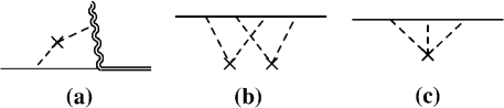
Figure 2: Examples of (a) bridging, (b) crossing diagrams, and (c) higher order terms neglected in the calculation.

         

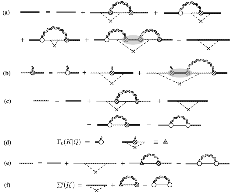
Figure 3: Feynman diagrams for the impurity dressed full Green’s function.

To address the impurity scattering, we begin at the Abrikosov-Gor’kov (AG) level,Abrikosov and Gor’kov (1959, 1960); AGD which is a good approximation in the Born limit. Following AG, we include all possible configurations of impurity dressing, but excluding bridging diagrams like Fig. 2(a), crossing diagrams like Fig. 2(b), and higher order terms like Fig. 2(c). The dashed lines denote impurity scattering, and the crosses denote the impurity vertices. We clarity, in most diagrams, we do not draw the fermion propagation arrows. It is understood, however, that they change direction at and only at a pairing vertex. As in subsec. II.1, we use plain double lines to denote the Green’s function ($G^{0}$) fully dressed by the pairing interaction but without impurity scattering, i.e.,

$$G^{0}(K)=\frac{1}{i\omega-\epsilon_{\bf k}-\Sigma^{0}(K)}\;,$$ (11)

where

$$\Sigma^{0}(K)=\sum_{Q}t(Q)G^{0}_{0}(Q-K)\varphi_{{\mathbf{k}}-{\mathbf{q}}/2}^{2}\;.$$ (12)

However, since we will address the impurity dressing of the pairing vertex or, equivalently, the pair susceptibility $\chi(Q)$, we assume the pair propagator $t(Q)$ in the above equation is already dressed with impurity scattering, with

$$t(Q)=t_{sc}(Q)+t_{pg}(Q)\;,$$ (13)

$$t_{sc}(Q)=-\frac{\Delta_{sc}^{2}}{T}\delta(Q)\;,$$ (14)

and

$$\Delta_{pg}^{2}=-\sum_{Q\neq 0}t_{pg}(Q)=-\sum_{Q\neq 0}\frac{g}{1+g\chi(Q)}\>,$$ (15)

as in the clean case. The shaded double lines denote impurity-dressed full Green’s function $G$, and “shaded” single lines denote impurity-dressed bare Green’s function (which we call $\hat{G}_{0}$), i.e,

$$\hat{G}_{0}(K)=\frac{1}{i\omega-\epsilon_{\bf k}-\bar{\hat{G}}_{0,\omega}}\;,$$ (16)

where the bar denotes impurity average $\bar{\hat{G}}_{0,\omega}=n_{i}\sum_{\bf k^{\prime}}|u(\textbf{k}-\textbf{k}^{\prime})|^{2}\hat{G}_{0}(K^{\prime})$. We use open circles to denote bare pairing vertex $\gamma(K|Q)=\varphi_{{\mathbf{k}}+{\mathbf{q}}/2}$, and shaded circles full pairing vertex $\Gamma(K|Q)$, where $Q$ is the pair four-momentum. To obtain the Feynman diagrams for the impurity dressed full $G$, we first expand the pairing self-energy diagram as an infinite series which contains only bare single particle Green’s function and pair propagators, and then insert all possible impurity scattering on the single particle propagators at the AG level. We assume that the pair propagators are always self-consistently dressed by the impurity scattering. After regrouping all non-impurity dressed lines on the left, the final result for the diagrams is shown in Fig. 3(a). Here following AG, the subdiagrams inside the two impurity legs are assumed to be self-consistently dressed by impurity scattering. To make direct comparison with the BCS case easier, we present the corresponding diagrams for the BCS case in Appendix A. The first term on the right hand side (RHS) of Fig. 3(a) contains all diagrams without impurity dressing (except via the pair propagators). The second term corresponds to the third term of the first equation in Fig. 18. The third term corresponds to the last term, the last term to the second. The fourth and the fifth together correspond to the fourth term [see Fig. 4(a)]. The fifth term in Fig. 3(a) arises since the two impurity legs can cross two separate pairing self-energy dressing parts; it can be eliminated using the equality shown in Fig. 3(b). Here the shaded elliptical region denotes self-consistent impurity dressing of the double pairing vertex structure inside the two impurity scattering legs, as shown in Fig. 4(a). It is worth pointing out that these diagrams reduce to their BCS counterpart if one removes the pairing propagators. The Dyson’s equation $\hat{G}_{0}^{-1}(K)={G_{0}^{0}}^{-1}(K)-\bar{\hat{G}}_{0,\omega}$ can then be used to eliminate the fourth term in Fig. 3(a). We now obtain the greatly simplified diagrams for $G$ as shown in Fig. 3(c), which can be further reduced into Fig. 3(e), upon defining a reduced pairing vertex $\Gamma_{0}(K|Q)$ (shaded triangles) as shown in Fig. 3(d),

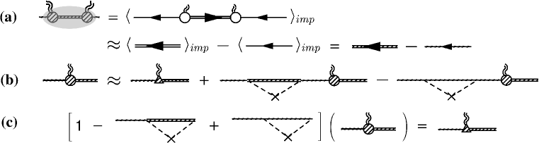
Figure 4: Feynman diagrams for pairing vertex.

$$\Gamma_{0}(K|Q) = \varphi_{{\mathbf{k}}-{\mathbf{q}}/2}$$ (17)

$$\hskip-45.52458pt+n_{i}\sum_{\bf k^{\prime}}|u(\textbf{k}-\textbf{k}^{\prime})|^{2}\hat{G}_{0}(Q-K^{\prime})\Gamma(K^{\prime}|Q)G(K^{\prime})\;.$$

One can then read off the impurity-induced quasiparticle self-energy $\Sigma^{\prime}(K)={G^{0}}^{-1}(K)-G^{-1}(K)$ immediately, as shown in Fig. 3(e),

$$\Sigma^{\prime}(K)=\bar{G}_{\omega}+\Sigma(K)-\Sigma_{0}(K)\;,$$ (18)

where the impurity average

$$\bar{G}_{\omega}=n_{i}\sum_{\bf k^{\prime}}|u(\textbf{k}-\textbf{k}^{\prime})|^{2}G(K^{\prime})\;,$$ (19)

and the “full” self-energy

$$\Sigma(K)=\sum_{Q}\Gamma_{0}(K|Q)t(Q)\Gamma(K|Q)\hat{G}_{0}(Q-K)\;.$$ (20)

Therefore, we have finally

$$G^{-1}(K) = {G^{0}}^{-1}(K)-\Sigma^{\prime}(K)=i\omega-\epsilon_{\mathbf{k}}-\bar{G}_{\omega}-\Sigma(K)$$ (21)

$$= i\tilde{\omega}-\epsilon_{\mathbf{k}}-\Sigma(K)=G_{0}^{-1}(K)-\Sigma(K)\;,$$

where we have defined the renormalized frequency $i\tilde{\omega}=i\omega-\bar{G}_{\omega}$ and the “bare” Green’s function

$$G_{0}(K)=\frac{1}{i\tilde{\omega}-\epsilon_{\mathbf{k}}}\;.$$ (22)

Note here $G_{0}(K)\neq\hat{G}_{0}(K)$.

Now we deal further with the pairing vertex $\Gamma(K|Q)$. First, we notice that the impurity-dressed double-vertex structure in Fig. 3(a) can be simplified as shown in Fig. 4(a) using the approximation

$$\sum_{Q}t(Q)f(K,Q)\approx\bigg{[}\sum_{Q}t(Q)\bigg{]}f(K,0)\;,$$ (23)

where $f(K,Q)$ is an arbitrary slow-varying function of $Q$. This is due to the fact that $t(Q)$ diverges as $Q\rightarrow 0$ at $T\leq T_{c}$. The Dyson’s equation for the Green’s function $G^{0}(-K)$ in a clean system is also used in getting the second line of Fig. 4(a). Therefore, we have approximately the impurity-dressed pairing vertex as shown in Fig. 4(b), which implies the equality shown in Fig. 4(c). Fig. 4(c) can be written as

$$\hat{G}_{0}(K)\Gamma(K|Q)G(Q-K) = \frac{\Gamma_{0}(K|Q)G(Q-K)}{\hat{G}_{0}^{-1}(K)-\bar{G}_{\omega}+\bar{\hat{G}}_{0,\omega}}$$ (24)

$$\hskip-50.58878pt=G_{0}(K)\Gamma_{0}(K|Q)G(Q-K)\;.$$

This result demonstrates the following important relationship:

$$\hat{G}_{0}(K)\Gamma(K|Q)=G_{0}(K)\Gamma_{0}(K|Q),\quad(\mbox{small\ }Q)\;.$$ (25)

Using this relationship, now the self-energy can be simplified as follows:

$$\Sigma(K) = \sum_{Q}\Gamma_{0}^{2}(K|Q)t(Q)G_{0}(Q-K)$$ (26)

$$\approx -\Delta^{2}\Gamma_{0}^{2}(K)G_{0}(-K)=-\tilde{\Delta}_{\bf k}^{2}G_{0}(-K)\;,$$

where $\Gamma_{0}(K)\equiv\Gamma(K|Q=0)$ and $\tilde{\Delta}_{\bf k}=\Delta\Gamma_{0}(K)$.

Finally, the impurity dressing of each rung [i.e., $\chi(Q)$] of the particle-particle scattering ladder diagrams is topologically identical to the impurity dressing of the pairing vertex and the two associated single particle lines. And summing up all the ladders gives the pairing $T$ matrix. Therefore, the pair susceptibility becomes

$$\chi(Q) = \sum_{K}\Gamma(K|Q)\hat{G}_{0}(Q-K)G(K)\varphi_{{\mathbf{k}}-{\mathbf{q}}/2}$$ (27)

$$\approx\sum_{K}\Gamma_{0}(K|Q)G_{0}(Q-K)G(K)\varphi_{{\mathbf{k}}-{\mathbf{q}}/2}\;.$$

And the gap equation is given by

$$1+g\chi(0)=0=1+g\sum_{K}\Gamma_{0}(K)G(K)G_{0}(-K)\varphi_{\mathbf{k}}\;.$$ (28)

This result can be easily verified to be consistent with the self-consistency condition. Define formally the generalized Gor’kov $F$ function:

$$F^{\dagger}(K)\equiv\Delta\hat{G}_{0}(-K)\Gamma(K)G(K)\;.$$ (29)

Using Eq. (25), we have

$$F^{\dagger}(K)\equiv\Delta\Gamma_{0}(K)G_{0}(-K)G(K)=\tilde{\Delta}_{\bf k}G_{0}(-K)G(K)\;.$$ (30)

The formal difference between this $F^{\dagger}$ and that in BCS is that $\varphi_{\mathbf{k}}$ is now replaced by the renormalized vertex $\Gamma_{0}(K)$. One immediately sees that the condition

$$\Delta_{\bf k}\equiv-g\sum_{K^{\prime}}\varphi_{\mathbf{k}}\varphi_{\bf k^{\prime}}F^{\dagger}(K^{\prime})$$ (31)

is consistent with the gap equation Eq. (28). However, it should be emphasized that the $F$ function so defined does not vanish above $T_{c}$ in the pseudogap regime, different from the BCS case.

II.3 Impurity scattering beyond the AG level

In this subsection, we include both the impurity scattering $T$-matrix with the particle-particle scattering $T$-matrix, and, thus, go beyond the AG level. We notice that if one replaces the second-order impurity scattering subdiagrams at the AG level with the corresponding impurity $T$-matrices, as shown in Fig. 5, the derivation for $G(K)$ goes through formally without modification. Now we only need to determine the impurity $T$-matrices $T_{\omega}$ and $T_{\Delta^{\dagger}}$ (as well as their complex conjugate) in terms of their AG-level counterpart, $\bar{G}_{\omega}$ and $\bar{F}^{\dagger}_{\omega}=n_{i}\sum_{\bf k^{\prime}}|u({\bf k-k^{\prime}})|^{2}F^{\dagger}(K^{\prime})$, respectively. In other words, except that $i\tilde{\omega}$ and $\tilde{\Delta}_{\bf k}$ now have different expressions, everything else remains the same in terms of $i\tilde{\omega}$ and $\tilde{\Delta}_{\bf k}$ (as well as their complex conjugate), just as in the BCS case (see Appendix A).

Figure 5: Replacement scheme from the AG level to self-consistent impurity $T$-matrix treatment.

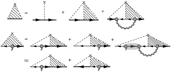
Figure 6: Relationship between the regular impurity $T$-matrix $T_{\omega}$ and the anomalous impurity $T$-matrix $T_{\Delta^{\dagger}}$.

The Feynman diagrams for $T_{\omega}$ and $T_{\Delta^{\dagger}}$ are shown in Fig. 6. To obtain the second line for $T_{\Delta^{\dagger}}$, we make use of the approximation in Fig. 4(a) to convert the left part of the second and the third term on the first line to the full $G$. This result is direct analogy with its BCS counterpart as shown in Fig. 20. One can now write down the equations for $T_{\omega}$ and $T_{\Delta^{\dagger}}$ without difficulty.

$$T_{\omega}({\mathbf{k}},{\mathbf{k}}^{\prime}) = u({\mathbf{k}},{\mathbf{k}}^{\prime})+\sum_{\bf k^{\prime\prime}}u({\mathbf{k}},{\mathbf{k}}^{\prime\prime})G(K^{\prime\prime})T_{\omega}({\mathbf{k}}^{\prime\prime},{\mathbf{k}}^{\prime})$$ (32)

$$+\sum_{\bf k^{\prime\prime}}\sum_{Q}u({\mathbf{k}},{\mathbf{k}}^{\prime\prime})G(K^{\prime\prime})\hat{G}_{0}(Q-K^{\prime\prime})$$

$${}\times\Gamma(K^{\prime\prime}|Q)t(Q)T_{\Delta^{\dagger}}(K^{\prime\prime}-Q,K^{\prime}|Q)\;,$$

and

$$T_{\Delta^{\dagger}}(K-Q,K^{\prime}|Q)=\sum_{\bf k^{\prime\prime}}u({\mathbf{k}}^{\prime\prime}-{\mathbf{q}},{\mathbf{k}}-{\mathbf{q}})$$

$${}\times\hat{G}_{0}(Q-K^{\prime\prime})G(K^{\prime\prime})\Gamma(K^{\prime\prime}|Q)T_{\omega}({\mathbf{k}}^{\prime\prime},{\mathbf{k}}^{\prime})$$

$$+\sum_{\bf k^{\prime\prime}}u({\mathbf{k}}^{\prime\prime}-{\mathbf{q}},{\mathbf{k}}-{\mathbf{q}})G(Q-K^{\prime\prime})T_{\Delta^{\dagger}}(K^{\prime\prime}-Q,K^{\prime}|Q)\,.$$

Note here $T_{\Delta^{\dagger}}$ does not contain the factor $\Delta$, unlike its BCS counterpart. It has the same dimension as $\Gamma$. Both $\Gamma$ and $\Gamma_{0}$ now contain the full impurity $T$-matrix beyond the AG level, and the vertex relation Eq. (25) remains valid. The new expression for $\Gamma_{0}$ is given by

$$\Gamma_{0}(K|Q)=\varphi_{{\mathbf{k}}-{\mathbf{q}}/2}+n_{i}\sum_{{\mathbf{k}}^{\prime}}T_{\Delta^{\dagger}}(K-Q,K^{\prime}|Q)\>.$$ (34)

So far, we have kept the derivation for a generic elastic scattering $u({\mathbf{k}},{\mathbf{k}}^{\prime})$. For isotropic $s$-wave scattering, $u({\mathbf{k}},{\mathbf{k}}^{\prime})=u$. In this case, $T_{\omega}$ and $T_{\Delta^{\dagger}}$ are independent of ${\mathbf{k}}$ and ${\mathbf{k}}^{\prime}$. Neglecting the momentum dependence, we obtain

$$T_{\Delta^{\dagger}}(\omega-\Omega,\omega)=\frac{u\sum_{\bf k}G_{0}(Q-K)\Gamma_{0}(K|Q)G(K)}{1-u\sum_{\bf k}G(Q-K)}T_{\omega}\;,$$ (35a)

and

$$T_{\omega} = u+u\sum_{{\mathbf{k}}}G(K)T_{\omega}$$ (35b)

$${}+u\sum_{Q}t(Q)\bigg{[}\sum_{{\mathbf{k}}}G(K)\Gamma_{0}(K|Q)G_{0}(Q-K)\bigg{]}$$

$${}\times T_{\Delta^{\dagger}}(\omega-\Omega,\omega)\;.$$

Use has been made of the vertex relation Eq. (25). Here again, we need to make use of the approximation Eq. (23). Defining $\bar{\bar{G}}_{\omega}=\sum_{{\mathbf{k}}}G(K)$ and

$$\bar{\bar{F}}^{\dagger}_{\omega}=\sum_{{\mathbf{k}}}F^{\dagger}(K)=\sum_{{\mathbf{k}}}\Delta\Gamma_{0}(K)G_{0}(-K)G(K)\,,$$ (36)

we obtain

$$T_{\omega}=\frac{u(1-u\bar{\bar{G}}_{-\omega})}{\left(1-u\bar{\bar{G}}_{\omega}\right)\left(1-u\bar{\bar{G}}_{-\omega}\right)+u^{2}\bar{\bar{F}}_{\omega}\bar{\bar{F}}^{\dagger}_{\omega}}\,,$$ (37a)

and

$$T_{\Delta^{\dagger}}(\omega-\Omega,\omega) = \frac{u^{2}\sum_{\bf k}G_{0}(Q-K)\Gamma_{0}(K|Q)G(K)}{\left(1-u\bar{\bar{G}}_{\omega}\right)\left(1-u\bar{\bar{G}}_{-\omega}\right)+u^{2}\bar{\bar{F}}_{\omega}\bar{\bar{F}}^{\dagger}_{\omega}}$$ (37b)

$${}\times\frac{1-u\bar{\bar{G}}_{-\omega}}{1-u\bar{\bar{G}}_{\Omega-\omega}}\,.$$

Letting $$\Omega\rightarrow 0$$, the last equation becomes

$$\Delta T_{\Delta^{\dagger}}(\omega)=\frac{u^{2}\bar{\bar{F}}^{\dagger}_{\omega}}{\left(1-u\bar{\bar{G}}_{\omega}\right)\left(1-u\bar{\bar{G}}_{-\omega}\right)+u^{2}\bar{\bar{F}}_{\omega}\bar{\bar{F}}^{\dagger}_{\omega}}\,.$$ (37c)

The frequency and gap renormalizations are given by

$$i\tilde{\omega}=i\omega-\Sigma_{\omega}\,,\quad i\tilde{\underline{\omega}}=-i\omega-\Sigma_{-\omega}\,,$$ (38a)

$$\tilde{\Delta}_{\mathbf{k}}=\Delta_{\mathbf{k}}+\Sigma_{\Delta}\,,\quad\tilde{\Delta}_{\mathbf{k}}^{*}=\Delta_{\mathbf{k}}^{*}+\Sigma_{\Delta^{\dagger}}$$ (38b)

where $\Sigma_{\omega}=n_{i}T_{\omega}$ and $\Sigma_{\Delta}=n_{i}\Delta T_{\Delta}$. Here $\tilde{\underline{\omega}}=\widetilde{(-\omega)}$. The expression for $\chi(Q)$ remains the same as in previous subsection.

For $d$-wave, $T_{\Delta^{\dagger}}=T_{\Delta}=0$, and $\tilde{\Delta}_{\mathbf{k}}=\Delta_{\mathbf{k}}$. Then Eq. (37a) is greatly simplified,

$$T_{\omega}=\frac{u}{1-u\bar{\bar{G}}_{\omega}}\,.$$ (39)

The full Green’s function is given by

$$G(K)=\frac{i\tilde{\underline{\omega}}-\epsilon_{\mathbf{k}}}{(i\tilde{\omega}-\epsilon_{\mathbf{k}})(i\tilde{\underline{\omega}}-\epsilon_{\mathbf{k}})+\Delta_{\mathbf{k}}^{*}\Delta_{\mathbf{k}}}\,.$$ (40)

Due to the approximation Eq. (23), we are able to bring the final result Eqs. (39) and (40) into the BCS form. It is easy to show that they are equivalent to the more familiar form in Nambu formalism, as used in Ref. Hirschfeld et al., 1988. Define

$$T_{A\omega}=\frac{1}{2}(T_{\omega}-T_{-\omega}),\quad T_{S\omega}=\frac{1}{2}(T_{\omega}+T_{-\omega})\,,$$ (41)

and similarly for $\Sigma_{\omega}$ and $\bar{\bar{G}}_{\omega}$. Here the subscript “A” and “S” denote antisymmetric and symmetric part, respectively. Further define

$$i\tilde{\omega}_{A}=i\omega-\Sigma_{A\omega},\quad\tilde{\epsilon}_{K}=\epsilon_{\mathbf{k}}+\Sigma_{S\omega}\,,$$ (42)

then we obtain (with $\Delta^{*}=\Delta$)

$$G(K)=\frac{i\tilde{\omega}_{A}+\tilde{\epsilon}_{K}}{(i\tilde{\omega}_{A})^{2}-\tilde{\epsilon}_{K}^{2}-\Delta_{\mathbf{k}}^{2}}\,,$$ (43)

and

$$T_{A\omega} = \frac{u^{2}\bar{\bar{G}}_{A\omega}}{(1-u\bar{\bar{G}}_{S\omega})^{2}-u^{2}\bar{\bar{G}}_{A\omega}^{2}}\;,$$ (44a)

$$T_{S\omega} = \frac{u(1-\bar{\bar{G}}_{S\omega})}{(1-u\bar{\bar{G}}_{S\omega})^{2}-u^{2}\bar{\bar{G}}_{A\omega}^{2}}\;,$$ (44b)

where

$$\bar{\bar{G}}_{A\omega} = \sum_{\mathbf{k}}\frac{i\tilde{\omega}_{A}}{(i\tilde{\omega}_{A})^{2}-\tilde{\epsilon}_{K}^{2}-\Delta_{\mathbf{k}}^{2}}\,,$$ (45a)

$$\bar{\bar{G}}_{S\omega} = \sum_{\mathbf{k}}\frac{\tilde{\epsilon}_{K}}{(i\tilde{\omega}_{A})^{2}-\tilde{\epsilon}_{K}^{2}-\Delta_{\mathbf{k}}^{2}}\,,$$ (45b)

are the antisymmetric and symmetric parts of $\bar{\bar{G}}_{\omega}$, respectively. It is evident that $T_{A}$ and $T_{S}$ correspond to $T_{0}$ and $-T_{3}$, respectively, in the Nambu formalism in Ref. Hirschfeld et al., 1988, (and similarly for $G_{A}$ and $G_{S}$).

It should be emphasized, however, that unless $u=0$ or $u=\pm\infty$, the symmetric part of the impurity $T$-matrix, $T_{S\omega}$, can never be set to zero, even if one could in principle have $\bar{\bar{G}}_{S\omega}=0$. This means that $\tilde{\epsilon}_{K}$ will always acquire a non-trivial, frequency dependent renormalization, $\Sigma_{S\omega}$. While this renormalization is small for weak coupling BCS superconductors, it is expected to be significant for the cuprate superconductors.

III Numerical solutions for $d$-wave superconductors

III.1 Analytical continuation and equations to solve

Since there is no explicit pairing vertex renormalization for $d$-wave superconductors, i.e., $\Gamma_{0}(K)=\varphi_{\mathbf{k}}$ or $\tilde{\Delta}_{\mathbf{k}}=\Delta_{\mathbf{k}}$, a major part of the numerics is to calculate the frequency renormalization. Everything else will follow straightforwardly.

Numerical calculations can be done in the real frequencies, after proper analytical continuation. Since $T_{S\omega}\neq 0$, $\Sigma_{\omega}$ and $\Sigma_{-\omega}$ are independent of each other. To obtain the frequency renormalization $\Sigma_{\omega}$, one has to solve a set of four equations for $\bar{\bar{G}}_{\omega}$, $\bar{\bar{G}}_{-\omega}$, $\Sigma_{\omega}$, and $\Sigma_{-\omega}$ self-consistently for given $\omega$. Because $i\tilde{\underline{\omega}}\neq-i\tilde{\omega}$, and one needs to analytically continue both simultaneously, the analytical continuation must be done carefully. For $n>0$, $i\tilde{\omega}_{n}\rightarrow\omega_{+}^{R}=\omega_{+}+i\Sigma^{\prime\prime}_{+}$, and $i\tilde{\underline{\omega}}_{n}\rightarrow\omega_{-}^{A}=\omega_{-}-i\Sigma^{\prime\prime}_{-}$. For $n^{\prime}=-n<0$, $i\tilde{\omega}_{n^{\prime}}\rightarrow\omega_{-}^{R}=\omega_{-}+i\Sigma^{\prime\prime}_{-}$ and $i\tilde{\underline{\omega}}_{n^{\prime}}\rightarrow\omega_{+}^{A}=\omega_{+}-i\Sigma^{\prime\prime}_{+}$. Here $\omega_{\pm}=\pm\omega-\Sigma^{\prime}_{\pm}$, and we choose $\omega>0$ and $\Sigma_{\pm}^{\prime\prime}>0$. Then we obtain four equations as follows:

$$\bar{\bar{G}}^{R}_{\omega>0} = \sum_{\mathbf{k}}\frac{\omega_{-}-i\Sigma_{-}^{\prime\prime}-\epsilon_{\mathbf{k}}}{(\omega_{+}+i\Sigma_{+}^{\prime\prime}-\epsilon_{\mathbf{k}})(\omega_{-}-i\Sigma_{-}^{\prime\prime}-\epsilon_{\mathbf{k}})+\Delta^{2}_{\mathbf{k}}}$$

$$\bar{\bar{G}}^{R}_{-\omega<0} = \sum_{\mathbf{k}}\frac{\omega_{+}-i\Sigma_{+}^{\prime\prime}-\epsilon_{\mathbf{k}}}{(\omega_{-}+i\Sigma_{-}^{\prime\prime}-\epsilon_{\mathbf{k}})(\omega_{+}-i\Sigma_{+}^{\prime\prime}-\epsilon_{\mathbf{k}})+\Delta^{2}_{\mathbf{k}}}$$

$$\Sigma^{R}_{\omega>0} = \frac{n_{i}u}{1-u\bar{\bar{G}}^{R}_{\omega}}=\Sigma_{+}^{\prime}-i\Sigma_{+}^{\prime\prime}$$

$$\Sigma^{R}_{-\omega>0} = \frac{n_{i}u}{1-u\bar{\bar{G}}^{R}_{-\omega}}=\Sigma_{-}^{\prime}-i\Sigma_{-}^{\prime\prime}$$ (46)

These equations are solved self-consistently for $(\Sigma^{\prime}_{\pm},\Sigma^{\prime\prime}_{\pm})$, as well as the real and imaginary parts of $\bar{\bar{G}}_{\pm\omega}$, as a function of $\omega$. No Kramers-Kronig relations are invoked in these numerical calculations. Note in real numerics, we subtract $\Sigma^{\prime}_{\omega=0}$ from $\Sigma^{R}_{\omega}$ so that $\Sigma^{\prime}_{\omega=0}=0$. This subtraction is compensated by a constant shift in the chemical potential $\mu$.

Having solved the frequency renormalization $\Sigma_{\omega}$, one can evaluate the pair susceptibility in the gap equation Eq. (28),

$$\chi(0)=\sum_{K}\frac{\varphi_{\mathbf{k}}^{2}}{(i\tilde{\omega}-\epsilon_{\mathbf{k}})(i\tilde{\underline{\omega}}-\epsilon_{\mathbf{k}})+\Delta^{2}_{\mathbf{k}}}$$

$$=\mbox{Im}\sum_{\mathbf{k}}\int_{0}^{\infty}\frac{d\omega}{\pi}\frac{[1-2f(\omega)]\>\varphi_{\mathbf{k}}^{2}}{(\omega_{+}+i\Sigma_{+}^{\prime\prime}-\epsilon_{\mathbf{k}})(\omega_{-}-i\Sigma_{-}^{\prime\prime}-\epsilon_{\mathbf{k}})+\Delta^{2}_{\mathbf{k}}}\,,$$

where $f(x)$ is the Fermi distribution function. It is easy to check that the gap equation Eq. (28) does reduce to its clean counterpart Eq. (7) as $n_{i}\rightarrow 0$.

The particle number equation becomes

$$n=2\sum_{\mathbf{k}}\int_{-\infty}^{\infty}\frac{d\omega}{2\pi}A({\mathbf{k}},\omega)f(\omega)=-2\,\mathrm{Im}\int_{-\infty}^{\infty}\frac{d\omega}{\pi}\bar{\bar{G}}^{R}_{\omega}f(\omega)\,.$$ (48)

The real and imaginary parts of $\chi(Q)$ are given respectively by

$$\chi^{\prime}(\Omega+i0^{+},{\mathbf{q}})$$ (49a)

$${}=\mbox{Im}\sum_{\mathbf{k}}\int_{-\infty}^{\infty}\frac{d\omega}{2\pi}\Big{\{}G^{R}(\omega,{\mathbf{k}})G^{R}_{0}(\Omega-\omega,{\mathbf{q-k}})$$

$${}\times\left[f(\omega-\Omega)-f(\omega)\right]$$

$${}+G^{R}(\omega,{\mathbf{k}})G^{A}_{0}(\Omega-\omega,{\mathbf{q-k}})$$

$${}\times\left[1-f(\omega)-f(\omega-\Omega)\right]\Big{\}}\varphi_{{\mathbf{k}}-{\mathbf{q}}/2}^{2}\,,$$

and

$$\chi^{\prime\prime}(\Omega+i0^{+},{\mathbf{q}})$$ (49b)

$${}=-\sum_{\mathbf{k}}\int_{-\infty}^{\infty}\frac{d\omega}{2\pi}\mathrm{Im}\,G^{R}(\omega,{\mathbf{k}})A_{0}(\Omega-\omega,{\mathbf{q-k}})$$

$${}\times\left[f(\Omega-\omega)-f(\omega)\right]\varphi_{{\mathbf{k}}-{\mathbf{q}}/2}^{2}\,,$$

where $A_{0}(\omega,{\mathbf{k}})=-2\mbox{Im}\,G^{R}_{0}(\omega,{\mathbf{k}})$ is the “bare” spectral function.

The pseudogap is evaluated via Eq. (15). To this end, we expand the inverse $T$-matrix to the order of $\Omega$ and $q^{2}$ via a (lengthy but straightforward) Taylor expansion

$$t^{-1}_{pg}(\Omega+i0^{+},{\mathbf{q}}) = \chi(\Omega+i0^{+},{\mathbf{q}})-\chi(0,{\mathbf{0}})$$ (50)

$$= (a_{0}^{\prime}+ia_{0}^{\prime\prime})\Omega+b^{\prime}q^{2}+ia_{1}^{\prime\prime}\Omega^{2}\,.$$

Here the imaginary part $b^{\prime\prime}$ vanishes. The term $b^{\prime}q^{2}$ should be understood as $b^{\prime}_{\parallel}q_{\parallel}^{2}+b^{\prime}_{\perp}q_{\perp}^{2}$ for a quasi-two dimensional square lattice. We keep the imaginary part up to the $\Omega^{2}$ order. Substituting Eq. (50) into Eq. (15), we obtain

$$\Delta_{pg}^{2}=\sum_{\mathbf{q}}\int_{-\infty}^{\infty}\frac{d\Omega}{\pi}\frac{(a_{0}^{\prime\prime}+a_{1}^{\prime\prime}\Omega)\Omega}{(a_{0}^{\prime}\Omega+b^{\prime}q^{2})^{2}+(a_{0}^{\prime\prime}+a_{1}^{\prime\prime}\Omega)^{2}\Omega^{2}}b(\Omega)\,,$$ (51)

where $b(x)$ is the Bose distribution function.

Numerical solutions confirm that the coefficients $a^{\prime}_{0}$ and $b^{\prime}$ have very weak $T$ dependence at low $T$. Therefore, in a three-dimensional (3D) system, we have $\Delta_{pg}^{2}\sim T^{3/2}$ at low $T$. As the system dimensionality approaches two, the exponent decreases from $3/2$ to $1$. However, in most physical systems, e.g., the cuprates, this exponent is close to $3/2$. The product $n_{p}\equiv a_{0}^{\prime}\Delta_{pg}^{2}$ roughly measures the density of incoherent pairs.

The gap equation (28) [together with Eq. (LABEL:eq:chi-int)], the fermion number equation (48), and the pseudogap equation (51) form a closed set, which will be solved self-consistently for $T_{c}$, $\mu$, and gaps at and below $T_{c}$. For given parameters $T_{c}$, $\mu$, and gaps, we can calculate the frequency renormalization, $\Sigma_{\omega}$, and then solve the three equations. A equation solver is then used to search for the solution for these parameters. The momentum sum is carried out using integrals. Very densely populated data points of $\omega$ are used automatically where $\Sigma_{\omega}$ and/or $\bar{\bar{G}}_{\omega}$ change sharply. A smooth, parabolic interpolation scheme is used in the integration with respect to $\omega$. The relative error of the solutions is less than $1.0\times 10^{-5}$, and the equations are satisfied with a relative error on both sides less than $1.0\times 10^{-7}$. In this way, our numerical results are much more precise than those calculated on a finite size lattice.

The solutions of these equations can be used to calculate the superfluid density $n_{s}/m$. Without giving much details, we state here that the impurity dressing of the current vertex for the (short-coherence-length) cuprate superconductors does not lead to considerable contributions for $s$-wave isotropic scattering and the long wavelength $q\rightarrow 0$ limit. The expression for the in-plane $n_{s}/m$ is given formally by the formula for a clean system (before the Matsubara summation is carried out), as in Ref. Kosztin et al., 2000,

$$\frac{n_{s}}{m}=\frac{n}{m}+P(0)\,,$$ (52)

where the in-plane current-current correlation function $P_{ij}(Q)=P(Q)\delta_{ij}$ can be simply derived from Eqs. (31) and (32) of Ref. Kosztin et al., 2000. The result is given by

$$P(Q) = \sum_{K}G(K)G(K-Q)\bigg{\{}\Big{[}1+(\Delta_{sc}^{2}-\Delta_{pg}^{2})\varphi_{\mathbf{k}}\varphi_{\mathbf{k-q}}$$ (53)

$${}\times G_{0}(-K)G_{0}(Q-K)\Big{]}\left(\frac{\partial\epsilon_{{\mathbf{k}}-{\mathbf{q}}/2}}{\partial{\mathbf{k}}_{\parallel}}\right)^{2}$$

$${}-\Delta_{pg}^{2}G_{0}(K)\frac{\partial\epsilon_{{\mathbf{k}}-{\mathbf{q}}/2}}{\partial{\mathbf{k}}_{\parallel}}\cdot\frac{\partial\varphi^{2}_{\mathbf{k}}}{\partial{\mathbf{k}}_{\parallel}}\bigg{\}}\,.$$

Using spectral representation and after lengthy but straightforward derivation, we obtain

$$\frac{n_{s}}{m} = 4\Delta_{sc}^{2}\sum_{\mathbf{k}}\int_{-\infty}^{\infty}\frac{d\omega}{2\pi}\;\mathrm{Im}\left[\left(\tilde{F}^{A}(\omega,{\mathbf{k}})\right)^{2}(\vec{\nabla}\epsilon_{\mathbf{k}})^{2}\varphi_{\mathbf{k}}^{2}\right.$$ (54)

$${}+\left.\frac{1}{2}G^{A}(\omega,{\mathbf{k}})\tilde{F}^{A}(\omega,{\mathbf{k}})\vec{\nabla}\epsilon_{\mathbf{k}}\cdot\vec{\nabla}\varphi^{2}_{\mathbf{k}}\right]f(\omega)\,,$$

where

$$\tilde{F}(K)=G(K)G_{0}(-K)=\frac{1}{(i\tilde{\omega}-\epsilon_{\mathbf{k}})(i\tilde{\underline{\omega}}-\epsilon_{\mathbf{k}})+\Delta^{2}_{\mathbf{k}}}\,,$$ (55)

which differs from $F(K)$ by a factor $\Delta_{\mathbf{k}}$.

As in the clean system, Eq. (54) differs from its BCS counterpart $(n_{s}/m)_{BCS}$ only by the overall prefactor, $\Delta_{sc}^{2}$,

$$\frac{n_{s}}{m\;}=\frac{\Delta_{sc}^{2}}{\Delta^{2}}\left(\frac{n_{s}}{m}\right)_{BCS}\;.$$ (56)

For $d$-wave superconductors, $(n_{s}/m)_{BCS}\sim A-BT$ or $A-BT^{2}$ at very low $T$, depending on whether the system is clean or dirty. Bearing in mind that $\Delta_{sc}^{2}/\Delta^{2}=1-\Delta_{pg}^{2}/\Delta^{2}\sim 1-C^{\prime}T^{3/2}$, we have

$$\frac{n_{s}}{m} \sim A-BT-CT^{3/2}\;,\qquad\mbox{(clean)},$$ (57)

$$\sim A-BT^{2}-CT^{3/2},\qquad\mbox{(dirty)},$$

at very low $T$. In other words, pair excitations lead to a new $T^{3/2}$ term in the low $T$ superfluid density.

III.2 Renormalization of the frequency by impurity scattering and the density of states

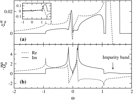
Figure 7: Example of (a) the frequency renormalization $-\Sigma_{\omega}^{R}$ and (b) impurity average of Green’s function $-\bar{\bar{G}}^{R}_{\omega}$ for a $d$-wave superconductor. The dashed and solid lines denote the real and imaginary parts, respectively. The full impurity band for $-\Sigma^{R}_{\omega}$ is shown in the inset. The parameters used are $\mu=0.92$, $t_{\perp}/t_{\parallel}=0.01$, $n_{i}=0.02$, $u=1$, $\Delta=0.08$. The energy unit is $4t_{\parallel}$, the half bandwidth.

Except in the Born limit, for $u\gtrsim 4t_{\parallel}$, impurity scattering usually introduces a sharp resonance close to the Fermi level in the frequency renormalization for a $d$-wave superconductor. In addition, it induces an impurity band outside the main particle band. Both the low energy resonance and the high energy impurity band arise from the vanishing of the real part of the denominator of the impurity $T$-matrix, Eq. (39), while the imaginary part is small. In Fig. 7 we show an example of (a) the retarded, impurity induced renormalization of the frequency, $-\Sigma^{R}_{\omega}=\tilde{\omega}^{R}-\omega$ and (b) the corresponding impurity average of the single-particle Green’s function, $-\bar{\bar{G}}^{R}_{\omega}$, which is related to the density of states by $N(\omega)=-2\,\mbox{Im}\,\bar{\bar{G}}^{R}_{\omega}$. The curves for $-\Sigma^{R}_{\omega}$ corresponding to the impurity band are replotted in the inset, to show the strong renormalization of the frequency inside the impurity band. (The curves for $-\Sigma^{\prime}_{\omega}$ has been offset so that $-\Sigma^{\prime}_{\omega=0}=0$. This offset is compensated by a shift in the chemical potential $\mu$.) The van Hove singularity and its mirror image via particle-hole mixing are clearly seen in the density of states, and are also reflected in $-\Sigma^{R}_{\omega}$ as the small kinks in Fig. 7(a). The real part $-\Sigma^{\prime}_{\omega}$ is usually neglected in most non-self-consistent calculations.Hirschfeld et al. (1988) It is evident, however, that it has a very rich structure, and, in general, cannot be set to zero in any self-consistent calculations. This conclusion holds even in the presence of exact particle-hole symmetry, as can be easily told from Eq. (39).

For $u<0$, the low energy resonance in $-\mbox{Im}\,\Sigma^{R}_{\omega}$ will appear on the positive energy side in Fig. 7(a). Regardless of the sign of $u$, the resonance peak will become sharper as $n_{i}$ decreases and as $|u|$ increases. For larger $|u|$, the resonant frequency will be closer to $\omega=0$, where $-\mbox{Im}\,\bar{\bar{G}}^{R}_{\omega}$ is small because of the $d$-wave symmetry; A smaller $n_{i}$ further reduces $-\mbox{Im}\,\bar{\bar{G}}^{R}_{\omega}$. Both factors help minimize the imaginary part of the denominator of Eq. (39) and, thus, lead to a stronger resonance. It should be emphasized that a resonance peak does not show up in $-\mbox{Im}\,\bar{\bar{G}}^{R}_{\omega}$ since the resonance in $-\mbox{Im}\,\Sigma^{R}_{\omega}$ requires that $-\mbox{Im}\,\bar{\bar{G}}^{R}_{\omega}$ be small at the resonance point.

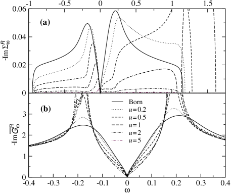
Figure 8: Evolution of (a) the frequency renormalization $-\mbox{Im}\,\Sigma_{\omega}^{R}$ and (b) impurity average of Green’s function $-\mbox{Im}\,\bar{\bar{G}}^{R}_{\omega}$ with $u$ for a $d$-wave superconductor at fixed $\gamma=n_{i}u^{2}=0.02$. A resonance develops in $-\mbox{Im}\,\Sigma_{\omega}^{R}$ as $u$ deviates from the Born limit. The weak scattering (Born limit) is more effective in filling in the DOS within the gap. The parameters used are $\mu=0.9$, $t_{\perp}/t_{\parallel}=0.01$, $\Delta=0.0945$.

The location of the impurity band is sensitive to the sign and strength of impurity scattering. For $u<0$, the impurity band on the negative energy (left) side of the plot. As $|u|$ gets smaller, the impurity band merges with the main band; as $|u|$ gets larger, it moves farther away, with a much stronger renormalization of $\omega$. For large $|u|$, the spectral weight under the impurity band in Fig. 7(b) is given by $2n_{i}$, and the weight in the main band is reduced to $2(1-n_{i})$. This leads to a dramatic chemical potential shift as a function of the impurity concentration $n_{i}$ (as well as $u$). For $u<0$, the impurity band will always be filled, so that increasing $n_{i}$ pushes the system farther away from the particle-hole symmetry. For $u>0$, on the contrary, the impurity band is empty, and the system becomes more particle-hole symmetrical as $n_{i}$ increases from 0, and reaches the particle-hole symmetry (in the main band) at $n_{i}=1-n$. This fact implies that Pépin and Lee’s assumption of an exact particle-hole symmetry is not justified so that their prediction of a diverging $N(\omega)$ as $\omega\rightarrow 0$ is unlikely to be observed experimentally. It should be mentioned that the appearance of the impurity band has not been shown in the literature, largely because most authors concentrate on the low energy part of the spectra only, and do not solve for the full spectrum of the renormalization of $\omega$ self-consistently.

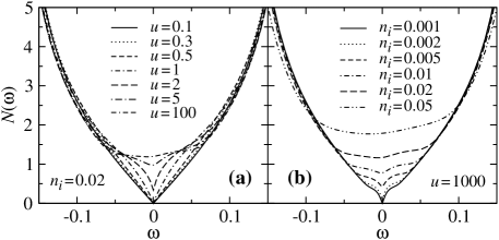
Figure 9: Evolution of the DOS $N(\omega)$ for a $d$-wave superconductor (a) with $u$ at $n_{i}=0.02$ and (b) with $n_{i}$ in the unitary limit $u=1000$. There is a dip at $\omega=0$ for small $n_{i}$ or small $u$. The parameters used are $\mu=0.9$, $t_{\perp}/t_{\parallel}=0.01$, $\Delta=0.0945$.

In the Born limit, only the product $\gamma=n_{i}u^{2}$ is a meaningful parameter, not $n_{i}$ or $u$ separately. In Fig. 8, we plot (a) the frequency renormalization $-\mbox{Im}\,\Sigma_{\omega}^{R}$ and (b) the impurity average of Green’s function $-\mbox{Im}\,\bar{\bar{G}}^{R}_{\omega}$ as a function of $\omega$ for various values of $u$ but with a fixed $\gamma=0.02$. (Note: when $u$ is small, this requires an unphysically large $n_{i}$.) In the Born limit, these two quantities are identical up to a constant coefficient. As $u$ increases, a resonance develops in $-\mbox{Im}\,\Sigma_{\omega}^{R}$ at small $\omega$. $-\mbox{Im}\,\Sigma_{\omega}^{R}$ and $-\mbox{Im}\,\bar{\bar{G}}^{R}_{\omega}$ become very different. And a impurity band develops gradually ($u=0.2$ and $u=0.5$), until it splits from the main band ($u=1$). At fixed $\gamma$, the Born limit is more effective in filling in the DOS in the mid-range of $\omega$ within the gap and smearing out the coherence quasiparticle peaks, whereas the large $u$ limit is more effective in filling in the DOS in the vicinity of $\omega=0$ but keeping the quasiparticle peaks largely unchanged. In addition, the main band becomes narrower at large $u$ than that in the clean system or the Born limit, so that part of the spectral weight has now been transferred to the impurity band. Also note that the DOS at $\omega=0$ is essentially zero in Fig. 8(b) because $n_{i}$ is very small when $u$ becomes large for the current choice of $\gamma=0.02$.

The effects of the scattering strength $u$ and the impurity density $n_{i}$ on the DOS are shown in Fig. 9(a) and (b), respectively. For the effect of $u$ in Fig. 9(a), we choose an intermediate $n_{i}=0.02$. And for the effect of $n_{i}$, we focus on the unitary limit, and choose $u=1000$. There is a dip in the DOS at $\omega=0$ in both the small $u$ and small $n_{i}$ cases, mimicking a fractional power law dependence on $\omega$. At higher $n_{i}$ and higher $u$, the DOS is filled in mainly at small $\omega$.

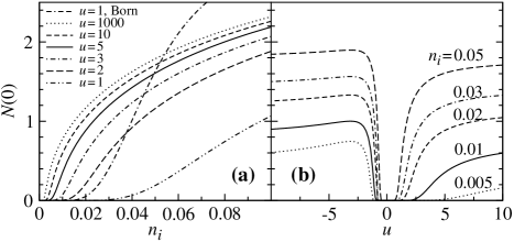
Figure 10: Residue DOS $N(0)$ at the Fermi level as a function of (a) $n_{i}$ for $u=1000$, 10, 5, 3, 2, and 1, and of (b) $u$ for $n_{i}=0.005$, 0.01, 0.02, 0.03, and 0.05. Also plotted in (a) is $N(0)$ as a function of $\gamma(=n_{i})$ in the Born limit. The parameters used are $\mu=0.9$, $t_{\perp}/t_{\parallel}=0.01$, $\Delta=0.0945$.

Shown in Fig. 10 are the residue DOS at the Fermi level, $N(0)$, as a function of (a) the impurity concentration $n_{i}$ for different values of $u$ from the unitary limit $u=1000$ through $u=10$, 5, 3, 2, down to 1, and (b) as a function of the scattering strength $u$ for $n_{i}=0.005$, 0.01, 0.02, 0.03, and 0.05. Figure 10(a) indicates that below certain “critical” value of $n_{i}$, $N(0)$ remains essentially zero. This behavior is also implied by the presence of the dip at small $n_{i}$ in Fig. 9(b). The “critical” value for $n_{i}$ in Fig. 10(a) is clearly scattering strength dependent. The smaller $u$, the larger this value. A replot (not shown) of these curves in terms of $\log_{10}N(0)$ as a function of $1/n_{i}$ reveals that for small $n_{i}$, $N(0)$ vanishes exponentially as $e^{-A/n_{i}}$, where $A$ is a constant. For comparison, we also show in Fig. 10(a) the Born limit as a function of $\gamma(=n_{i})$. As one may expect, the Born limit is rather different from the rest, since it is equivalent to a very small $u<<1$ and unphysically large $n_{i}$. A similar activation behavior of $N(0)$ as a function of $u$ is seen in Fig. 10(b), where the “critical” value for $u$ is strongly $n_{i}$ dependent. The asymmetry between positive and negative $u$ reflects the particle-hole asymmetry at $\mu=0.9$. It should be noted that it is not realistic to vary $u$ continuously in experiment.

An earlier experiment by Ishida et al.Ishida et al. (1993) suggests that $N(0)$ varies as $n_{i}^{1/2}$. In our calculations, however, $N(0)$ does not follow a simple power law as a function of $n_{i}$. The curve for $u=1000$ in Fig. 10(a) fits perfectly with $an_{i}^{\alpha}-b$, with $\alpha\approx 0.175$, for $0.002<n_{i}<0.05$. The damping of the zero frequency (not shown), $-\mbox{Im}\Sigma^{R}_{\omega=0}$, also fits this functional form very well, with $\alpha\approx 0.61$. The exponents are different for different values of $u$. Our calculation for the $n_{i}$ dependence of $N(0)$ is consistent with the result of FehrenbacherFehrenbacher (1996) in that $N(0,n_{i})$ it is strongly $u$ dependent. However, it does not seem likely that the simple power law $N(0)\sim n_{i}^{1/2}$ may be obtained in an accurate experimental measurement. Further experiments are needed to double check this relationship between $N(0)$ and $n_{i}$.

From Figs. 7-10, we conclude that for very small $n_{i}$ and $u$, the zero frequency DOS $N(0)$ is exponentially small. At high $n_{i}$, $N(0)$ is finite in both the Born and the unitary limit. However, for certain intermediate values of $n_{i}$ and $u$ [e.g., $u\sim 1$ in Fig. 9(a), and $n_{i}\lesssim 0.002$ in Fig. 9(b)], $N(\omega)$ vanishes with (very small) $\omega$ according to some fractional power $\omega^{\alpha}$ where $\alpha<1$. We see neither the universal power laws for $N(\omega)$ predicted by Senthil and Fisher,Senthil and Fisher (1999) nor the divergent DOS predicted by Pépin and LeePépin and Lee (2001) and others.Bocquet et al. (2000)

When the values of $u$ and $n_{i}$ are such that $N(\omega)\sim\omega^{\alpha}$ with $\alpha<1$, one may expect to see a fractional low $T$ power law in the superfluid density. However, such a power law is not robust as it is sensitive to the impurity density for a given type of impurity. The situation with a negative $u$ is similar to Fig. 9.

For given chemical potential $\mu$ and the total excitation gap $\Delta$, the calculation of the frequency renormalization with impurities does not necessarily involve the concept of the pseudogap. It is essentially the “self-consistent” impurity $T$-matrix treatment by Hirschfeld et al.Hirschfeld et al. (1988) except that we now have to solve for both the real and imaginary parts of $\Sigma_{\omega}^{R}$ simultaneously in a self-consistent fashion. Our numerical results agree with existing calculations in the literature.

Finally, we emphasize the difference between the self-consistent impurity $T$-matrix treatment of the one-impurity problem Kruis et al. (2001); Atkinson et al. (2000b) and the current many-impurity averaging. For the former case, the impurity $T$-matrix will be given by Eq. (37a) but with $\bar{\bar{G}}_{\omega}$ replaced by $\bar{\bar{G}}^{0}_{\omega}$, i.e., the impurity average of the clean $G^{0}(K)$. As a consequence, the position of the poles of $T_{\omega}$ is independent of the renormalized DOS, and, therefore, a resonance peak may exist at low $\omega$ in the DOS,Kruis et al. (2001) whereas it cannot in the current many-impurity case.

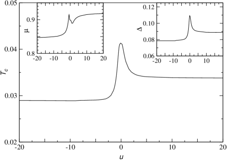
Figure 11: Behavior of $T_{c}$, $\mu$ (left inset), and $\Delta$ (right inset) as a function of the impurity scattering strength $u$ at $n=0.85$, $t_{\perp}/t_{\parallel}=0.01$, $-g/4t_{\parallel}=0.5$ and $n_{i}=0.05$.

III.3 Effects of the impurity scattering on $T_{c}$ and the pseudogap

In this section, we study the influence of impurity scattering on the behavior of $T_{c}$ and the pseudogap $\Delta_{pg}$ as a function of the coupling strength as well as the hole doping concentration.

First, we study the effect of the scattering strength $u$ and whether it is repulsive ($u>0$) or attractive ($u<0$). In Fig. 11, we plot $T_{c}$ as a function of $u$, for a pseudogapped $d$-wave superconductor with $n_{i}=0.05$. The corresponding curves for $\mu$ and $\Delta=\Delta_{pg}(T_{c})$ are shown in the upper left and upper right insets, respectively. All three quantities, $T_{c}$, $\mu$, and $\Delta$, vary with $u$. For either sign of $u$, both $T_{c}$ and $\Delta$ are suppressed by increasing $|u|$. It should be emphasized that the chemical potential $\mu$ in the two (large $\pm u$) unitary limits does not meet, nor does $T_{c}$ or $\Delta$. This is because a (large) negative $u$ creates a filled impurity band below the main band, and is effective in bringing down the chemical potential, whereas a positive $u$ creates an empty impurity band above the main band, and tends to raise $\mu$ toward the particle-hole symmetrical point, $\mu=1$. This result cannot and has not been observed in previous, non-self-consistent calculations where the real part of frequency renormalization is set to zero.

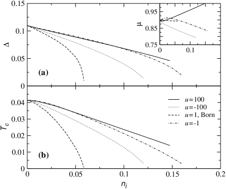
Figure 12: Evolution of (a) $\Delta_{pg}(T_{c})$, (b) $T_{c}$, and $\mu$ (inset), as a function of the impurity concentration $n_{i}$ for both positive ($u=100$) and negative ($u=-100$) scattering strength in the unitary limit, the Born limit ($u=1$, $\gamma=n_{i}$), and intermediate $u=-1$. Here $n=0.85$, $t_{\perp}/t_{\parallel}=0.01$, and $-g/4t_{\parallel}=0.5$.

In Fig. 12, we compare the effect of the impurity concentration for different scattering strengths: the Born limit, both unitary limits ($u=\pm 100$), and intermediate $u=-1$. Both (b) $T_{c}$ and (a) $\Delta_{pg}(T_{c})$ are suppressed by increasing impurity density. This is natural in a model where the pseudogap originates from incoherent pair excitations. As will be seen below, $\Delta_{pg}(T_{c})$ is suppressed mainly because $T_{c}$ is lowered. Except in the Born limit, the chemical potential $\mu$ is fairly sensitive to $n_{i}$, as shown in the inset. It is clear that the scattering in the Born limit is the most effective in suppressing $T_{c}$. In comparison with experiment,Franz et al. (1997) calculations at the AG level (i.e., the Born limit) tend to overestimate the $T_{c}$ suppression by as much as a factor of 2. This is in good agreement with the current result in the unitary limit. At large $n_{i}$ for large positive $u$, the system is driven to the particle-hole symmetrical point, where the effective pair mass changes sign. It is usually hard to suppress $T_{c}$ by pairing at the particle-hole symmetrical point, as indicated by the solid curve in the lower panel. In fact, exactly at this point, the linear $\Omega$ term $a_{0}^{\prime}$ in the inverse $T$ matrix expansion vanishes, so that one needs to go beyond the current approximation and expand up to the $\Omega^{2}$ term. Large negative $u=-100$ is more effective in suppressing $T_{c}$ and $\Delta$ than intermediate negative $u=-1$, in agreement with Fig. 11 and the DOS shown in Fig. 9(a) and Fig. 10.

There is enough evidence that zinc impurities are attractive scatterer for electrons in the cuprates.Fehrenbacher (1996) Therefore, we concentrate ourselves on negative $u$ scattering in the unitary limit. Plotted in Fig. 13 are $T_{c}$ (main figure), $\mu$ (lower inset), and $\Delta$ as a function of $g$ for increasing $n_{i}=0,0.02,0.05,0.1$ with $u=-100$. Also plotted for comparison are the results assuming the Born limit with $\gamma=0.05$. Clearly, the Born limit is more effective in suppressing $T_{c}$ at relatively weak coupling, $-g/4t_{\parallel}\lesssim 0.75$, consistent with Fig. 12. Both $T_{c}$ and $\Delta$ are suppressed continuously with $n_{i}$. However, it should be noted that a larger $n_{i}$ helps $T_{c}$ to survive a larger $-g/4t_{\parallel}$. This is mainly because the filled impurity band at large $n_{i}$ pushes the system far away from particle-hole symmetry (see $\mu$ in the lower inset), and reduces the effective fermion density, so that the pair mobility is enhanced and the pair mass does not diverge until a larger $-g/4t_{\parallel}$ is reached.

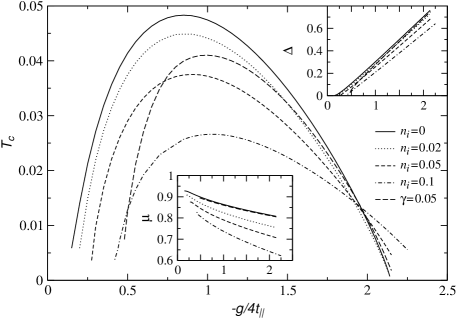
Figure 13: Behavior of $T_{c}$, $\mu$ (lower inset), and $\Delta$ (upper inset) as a function of $-g/4t_{\parallel}$ in the unitary limit for $u=-100$ and $n_{i}=0$ (solid curve), 0.02 (dotted), 0.05 (dashed), and 0.1 (dot-dashed). For comparison, curves for $\gamma=0.05$ in the Born limit are also plotted (long-dashed). Impurity scattering in the Born limit is more effective in suppressing $T_{c}$ at relatively weak coupling. The parameters are $n=0.85$, $t_{\perp}/t_{\parallel}=0.01$.

To make contact with the cuprates, we use the non-double occupancy condition associated with the Mott insulator physics, as in Ref. Chen et al., 1998, so that the effective hopping integral is reduced to $t_{\parallel}(x)\approx t_{0}x$, where $x=1-n$ is the hole concentration, and $t_{0}=0.6$ eV is the hopping integral in the absence of the on-site Coulomb repulsion. We assume $-g/4t_{0}=0.047$, which is $x$ independent. Then we can compute $T_{c}$, $\mu$, and $\Delta=\Delta_{pg}(T_{c})$ as a function of $x$. The result for $T_{c}$ (main figure) and $\Delta$ (inset) is shown in Fig. 14 for the clean system and $n_{i}=0.02$ and $0.05$. In the overdoped regime, $T_{c}$, as well as the small $\Delta$, are strongly suppressed by impurities. This provides a natural explanation for the experimental observation that $T_{c}$ vanishes abruptly at large $x$; it is well-known that high crystallinity, clean samples are not available in the extreme overdoped regime. On the other hand, neither $T_{c}$ nor $\Delta$ is strongly suppressed in the highly underdoped regime, where the gap is too large. At this point, experimental data in this extreme underdoped regime are still not available. Our result about the suppression of $T_{c}$ and $\Delta$ in the less strongly underdoped regime ($x>0.1$) are in agreement with experimental observationsWilliams et al. (1995, 1998) and other calculations.Franz et al. (1997)

It should be noted, however, that in our simple model, we do not consider the fact that disorder or impurities may reduce the dimensionality of the electron motion and thus suppress $T_{c}$. Furthermore, since induced local spin and Kondo effects have been observed near zinc sites in both zinc-doped YBCOMacFarlane et al. (2000); Bobroff et al. (1999) and zinc-doped Bi₂Sr_2-xLa_xCuO_6+δ,Hanaki et al. (2001) this raises an important question whether zinc can be treated as a nonmagnetic impurity.

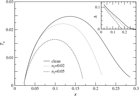
Figure 14: Behavior of $T_{c}$ and $\Delta$ (inset) as a function of the hole doping concentration $x$ in the unitary limit for $u=-100$ and $n_{i}=0$ (solid curve), 0.02 (dotted), and 0.05 (dashed). The parameters are $-g/4t_{0}=0.047$, $t_{\perp}/t_{\parallel}=0.003$.

III.4 Gaps and superfluid density below $T_{c}$ in the presence of nonmagnetic impurities

In this subsection, we study the effect of nonmagnetic impurities on the behavior of the excitation gap $\Delta$, the order parameter $\Delta_{sc}$, and the pseudogap $\Delta_{pg}$ as well as the chemical potential $\mu$ as a function of temperature in the superconducting phase. The numerical solutions for these quantities are then used to study the temperature dependence of the superfluid density $n_{s}/m$ at various impurity levels. We concentrate on the unitary limit, which is regarded as relevant to the cuprates. To be specific, we use $n=0.85$, $t_{\perp}/t_{\parallel}=0.01$, and $u=-100$ in the calculations presented below.

We first study the impurity effect in the BCS case, without the complication of the pseudogap. Plotted in Fig. 15 are the superfluid density $n_{s}/m$ (main figure) and the corresponding gap $\Delta$ in a $d$-wave BCS superconductor as a function of the reduced temperature $T/T_{c}^{0}$ for the clean system (solid curves), impurity density $n_{i}=0.02$ (dotted), and $n_{i}=0.05$ (dashed) at $-g/4t_{\parallel}=0.3$. Here $T_{c}^{0}=0.0416$ is the $T_{c}$ in the clean case. As expected, both $T_{c}$ and $\Delta(T)$, as well as $n_{s}/m$, are suppressed by impurity scattering. In agreement with experiment, the low $T$ normal fluid density is linear in $T$ in the clean case, and becomes quadratic in the two dirty cases.

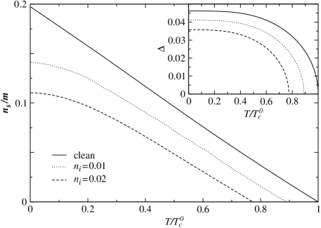
Figure 15: Behavior of the superfluid density $n_{s}/m$ and the excitation gap $\Delta$ (inset) in a $d$-wave BCS superconductor as a function of temperature $T/T_{c}^{0}$ for impurity concentration $n_{i}=0$ (clean, solid curve), 0.02 (dotted), and 0.05 (dashed) in the unitary limit $u=-100$. $T_{c}^{0}=0.0416$ is the $T_{c}$ in the clean system. The parameters are $n=0.85$, $-g/4t_{\parallel}=0.3$, and $t_{\perp}/t_{\parallel}=0.01$.

Now we add pseudogap for the underdoped cuprates. We show in Fig. 16 the temperature dependence of $n_{s}/m$ (main figure) and various gaps (inset) in a $d$-wave pseudogapped superconductor for impurity concentration $n_{i}=0$ (clean, solid curve), 0.02 (dotted), and 0.05 (dashed) in the unitary limit at $-g/4t_{\parallel}=0.5$. As the order parameter develops below $T_{c}$, the pseudogap decreases with decreasing $T$. This reflects the fact that the pseudogap in the present model is a measure of the density of thermally excited pair excitations. The total gap $\Delta$, the order parameter $\Delta_{sc}$, and the superfluid density $n_{s}/m$ are suppressed by increasing $n_{i}$, similar to the BCS case above. However, at given $T<T_{c}$, the pseudogap $\Delta_{pg}$ remains roughly unchanged. Furthermore, the low $T$ power law for the superfluid density is different from the BCS case, as predicted in Eq. (57). It is now given by $T+T^{3/2}$ and $T^{2}+T^{3/2}$ for the clean and dirty cases, respectively. Due to the presence of the $T^{3/2}$ term, the low $T$ portion of the curves for $n_{i}=0.02$ and 0.05 are clearly not as flat as in Fig. 15. Nevertheless, it may be difficult to distinguish experimentally $T^{2}+T^{3/2}$ from a pure $T^{2}$ power law. This $T^{3/2}$ contribution of the pair excitations has been used to explain successfullyChen et al. (1998) the quasi-universal behavior of the normalized superfluid density $n_{s}(T)/n_{s}(0)$ as a function of $T/T_{c}$. We have also foundChen et al. (2000b); Carrington et al. (1999) preliminary experimental support for this $T^{3/2}$ term in low $T$ penetration depth measurement in the cuprates as well as organic superconductors. Systematic experiments are needed to further verify this power law prediction.

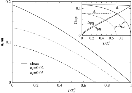
Figure 16: Behavior of the superfluid density $n_{s}/m$ and the various gaps (inset) in a $d$-wave pseudogapped superconductor as a function of temperature $T/T_{c}^{0}$ for impurity concentration $n_{i}=0$ (clean, solid curve), 0.02 (dotted), and 0.05 (dashed) in the unitary limit $u=-100$. Here $T_{c}^{0}=0.0414$. The parameters are $n=0.85$, $-g/4t_{\parallel}=0.5$, and $t_{\perp}/t_{\parallel}=0.01$.

A careful look at the values of the zero temperature superfluid density $(n_{s}/m)_{0}$ for different values of $n_{i}$ in both Fig. 15 and Fig. 16 suggests that in the unitary limit, $(n_{s}/m)_{0}$ drops faster with $n_{i}$ when $n_{i}$ is still small. This is manifested in a systematic study of $(n_{s}/m)_{0}$ as a function of $n_{i}$, as shown in Fig. 17, with $u=-100$ (solid curve). This behavior has been observed experimentally.Bernhard et al. (1996) Also plotted in the inset is the corresponding zero temperature gap $\Delta_{0}$ versus $n_{i}$. Clearly, the slope $d\frac{n_{s}}{m}/dn_{i}$ is much steeper as $n_{i}$ approaches zero, very different from the behavior of $\Delta_{0}$. This demonstrates that $n_{s}/m$ is influenced more by the DOS than by the gap size. A very small amount of impurities may strongly suppress $(n_{s}/m)_{0}$. This conclusion is significant in data analysis of the penetration depth measurement, especially when the $T=0$ value of penetration depth is not measured directly.Har For comparison, we also plot the corresponding curves in the Born limit. While the gap is suppressed faster, in contrast to unitary case, the slope $d\frac{n_{s}}{m}/dn_{i}$ is smaller for smaller $n_{i}$.

IV Discussion

In Sec. II, we have used the approximation Eq. (23) to bring the single-particle self-energy and thus the gap equation into a BCS-like form. This approximation derives from the divergence of the $T$ matrix $t_{pg}(Q)$ as $Q\rightarrow 0$, which is the pairing instability condition. The spirit of this approximation is to “put” the incoherent, excited pairs into the condensate, by setting $Q=0$. The contribution of these pseudo Cooper pairs to the single-particle excitation gap is calculated via Eqs. (15) and (51), weighted by the Bose function. Therefore, the incoherent pairs and the zero momentum condensate are not distinguished from each other in terms of the single particle self-energy, as they add up to a total excitation gap. However, they are distinct when phase sensitive quantities are involved, e.g., in the calculation of $T_{c}$ and of the superfluid density.

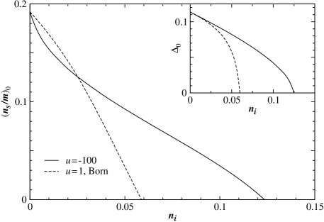
Figure 17: Zero temperature superfluid density $(n_{s}/m)_{0}$ and the gap $\Delta_{0}$ (inset) in a $d$-wave superconductor as a function of impurity concentration $n_{i}$ in the unitary limit ($u=-100$, solid line) and in the Born limit ($\gamma=n_{i}$, dashed line). The parameters are $n=0.85$, $-g/4t_{\parallel}=0.5$, and $t_{\perp}/t_{\parallel}=0.01$.

With this approximation, there is a close analogy between the Feynman diagrams in the current pairing fluctuation theory in Sec. II and its BCS counterpart in Appendix A. When the finite momentum pair propagators are removed (or “pushed into the condensate”) from Fig. 3 through Fig. 6, these diagrams will become their BCS counterpart in Fig. 18 through Fig. 20. (The diagram for BCS pairing vertex is not shown in Appendix A).

This approximation is in general good when the gap is large in comparison with $T$, and when the impurity concentration is low. When the gap is small, the contribution of the incoherent pair excitations is usually small, and does not have a strong effect on $T_{c}$, so that $T_{c}$ is roughly determined by its BCS mean-field solution. When $n_{i}$ is large, the fermionic frequency renormalization is strong, and the pair dispersion also becomes highly damped. In this case, approximation Eq. (23) may not be quantitatively accurate.

Even without the complication of impurities, incoherent pairs are not expected to deplete completely the spectral weight within the two quasiparticle peaks of the spectral function.Chen et al. (2001); Maly et al. (1999a) This, however, cannot be captured by the approximation Eq. (23). Unfortunately, we still do not know yet how to solve the Dyson’s equations without this approximation due to technical difficulties.

Another simplification comes from the $d$-wave symmetry of the cuprate superconductors under study. Although we have kept the theoretical formalism general for both $s$- and $d$-wave in Sec. II, the pairing vertex renormalization drops out when we finally carry out numerical calculations for $d$-wave superconductors. For $s$-wave superconductors, one would have to include self-consistently one more complex equation for the renormalization of $\Delta_{\mathbf{k}}$, when solving for the renormalization of $\omega$. And the equations (37a) and (37c) also look much more complicated than Eq. (39). Nevertheless, since there is no node in the excitation gap for $s$-wave, the numerics is expected to run faster.

It is well-known that for $d$-wave superconductors, the Anderson’s theoremAnderson (1959) breaks down.Gor’kov For Anderson’s theorem to hold, it requires that the gap and the frequency are renormalized in exactly the same fashion. This condition can be satisfied (approximately) only in weak coupling, isotropic BCS $s$-wave superconductors, for which the real part of the frequency renormalization is negligible. Since the frequency $\omega$ is a scalar, this condition is violated when the gap $\Delta_{\mathbf{k}}$ have any anisotropic dependence on k. Furthermore, when the gap is considerably large in comparison with the band width so that the upper limit of the energy integral cannot be extended to infinity, this condition will not be satisfied, either. In both cases, $T_{c}$ will be suppressed.

V Conclusions

In this paper, we extend the pairing fluction theory to superconductors in the presence of non-magnetic impurities. Both the pairing and impurity $T$-matrices are included and treated self-consistently. We obtain a set of three equations for ($T_{c}$, $\mu$, $\Delta(T_{c})$) or ($\mu$, $\Delta_{sc}$, $\Delta_{pg}$) at $T<T_{c}$, with the complex equations for the frequency renormalization. In consequence, we are able to study the impurity effects on $T_{c}$, the order parameter, and the pseudogap. In particular, we carry out calculations for $d$-wave superconductors and apply to the cuprate superconductors. Instead of studying the physical quantities with all possible combinations of the parameters $n_{i}$, $u$, $g$, and $n$, we mainly concentrate on the negative $u$ unitary limit, which is regarded as relevant to the zinc impurities in the cuprates.Fehrenbacher (1996)

Calculations show that in addition to the low energy resonance in the imaginary part of the renormalized frequency, a considerably large $|u|$ leads to a separate impurity band, with a spectral weight $2n_{i}$. The real part of the frequency renormalization, in general, cannot be set to zero in a self-consistent calculation. The chemical potential varies with the impurity concentration, so that the assumption of exact particle-hole symmetry is not justified when one studies the impurity effects. One consequence of this chemical potential shift is that the repulsive and attractive unitary scattering limits do not meet as has been widely assumed in the non-self-consistent treatment in the literature. Unitary scatterers fill in the DOS mostly in the small $\omega$ region, whereas Born scatterers do in essentially the whole range within the gap. At small $n_{i}$ and/or small $u$, there is a dip at $\omega=0$ in the DOS, so that $N(\omega)$ vanishes as a fractional power of $\omega$, which may in turn contribute a fractional power law for the low $T$ temperature dependence of the penetration depth.

Both $T_{c}$ and the pseudogap $\Delta_{pg}(T_{c})$ are suppressed by impurities. In this respect, Born scatterers are about twice as effective as unitary scatterer. Treating zinc impurities as unitary scatterers explains why the actual $T_{c}$ suppression is only half that predicted by calculations at the AG level (i.e., in the Born limit). In the overdoped regime, the gap is small, and therefore the superconductivity can be easily destroyed by a small amount of impurities. In contrast, it takes a larger amount of impurities to destroy the large excitation gap in the underdoped regime.

The reason $\Delta_{pg}(T_{c})$ is suppressed is mainly because $T_{c}$ is suppressed. In fact, for a given $T<T_{c}$, the pseudogap remains roughly unchanged (actually it increases slightly). The suppression of the total excitation gap arises from the suppression of the order parameter. The density of incoherent pairs, as measured by $n_{p}$, slightly increases for not-so-large $n_{i}$. This supports the notion that nonmagnetic impurities do not mainly break incoherent pairs. Instead, they scatter the Cooper pairs out of the condensate.Not

Our self-consistent calculations show that in the unitary limit, the low $T$ superfluid density is quadratic in $T$ in a BCS $d$-wave superconductor, in agreement with existing calculations and experiment. Strong pair excitations add an additional $T^{3/2}$ term, with preliminary experimental support. As a function of increasing $n_{i}$, the zero $T$ superfluid density decreases faster at first for unitary scatterers, whereas the opposite holds for scattering in the Born limit. The former behavior is in agreement with experiment.

Appendix A Impurity dressing for BCS theory at the Abrikosov-Gor’kov level

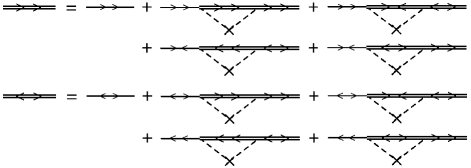
Figure 18: Impurity dressing at the Abrikosov-Gor’kov level in BCS theory.

In this appendix, we present the impurity dressing for a BCS superconductor, following Abrikosov-Gor’kovAbrikosov and Gor’kov (1959); AGD , but in a more general form, namely, we do not assume $\bar{G}_{-\omega}=-\bar{G}_{\omega}$. This will make it easier to understand the current theory in the presence of strong pairing correlations, as there is a strong similarity between the impurity dressing diagrams for both BCS theory and the pairing fluctuation theory.

For a pure BCS superconductor, we have the Gor’kov equations,

$${G^{0}_{0}}^{-1}(K)G^{0}(K)=1-\Delta_{\bf k}{F^{0}}^{\dagger}(K)\;,$$ (58a)

$${G^{0}_{0}}^{-1}(-K){F^{0}}^{\dagger}(K)=\Delta^{*}_{\bf k}G^{0}(K)\;.$$ (58b)

At the AG level, the relationship between the impurity dressed Green’s functions $G$ and $F$ is represented by the Feynman diagrams shown in Fig. 18. Define the impurity average $\bar{G}_{\omega}$ as in Eq. (19), and

$$\bar{F}^{\dagger}_{\omega}=n_{i}\sum_{\bf k^{\prime}}|u(\textbf{k}-\textbf{k}^{\prime})|^{2}F^{\dagger}(K^{\prime})\;,$$ (59)

as well as their complex conjugate. Note Fig. 18 is actually Fig. 105 in Ref. AGD, . Without giving details, we give the result following AG:

$$(i\omega-\epsilon_{\mathbf{k}}-\bar{G}_{\omega})G(K)+(\Delta_{\bf k}+\bar{F}_{\omega})F^{\dagger}(K)=1\,,$$ (60a)

$$(i\omega+\epsilon_{\mathbf{k}}+\bar{G}_{-\omega})F^{\dagger}(K)+(\Delta^{*}_{\bf k}+\bar{F}^{\dagger}_{\omega})G(K)=0\,.$$ (60b)

Define $i\tilde{\omega}=i\omega-\bar{G}_{\omega}$, $i\tilde{\underline{\omega}}=-i\omega-\bar{G}_{-\omega}$, $\tilde{\Delta}_{\bf k}=\Delta_{\bf k}+\bar{F}_{\omega}$, and $\tilde{\Delta}^{*}_{\bf k}=\Delta_{\bf k}^{*}+\bar{F}^{\dagger}_{\omega}$. Then we obtain

$$G(K)=\frac{i\tilde{\underline{\omega}}-\epsilon_{\mathbf{k}}}{(i\tilde{\omega}-\epsilon_{\mathbf{k}})(i\tilde{\underline{\omega}}-\epsilon_{\mathbf{k}})+\tilde{\Delta}_{\mathbf{k}}^{*}\tilde{\Delta}_{\mathbf{k}}}\,,$$ (61a)

$$F^{\dagger}(K)=\frac{\tilde{\Delta}^{*}_{\mathbf{k}}}{(i\tilde{\omega}-\epsilon_{\mathbf{k}})(i\tilde{\underline{\omega}}-\epsilon_{\mathbf{k}})+\tilde{\Delta}_{\mathbf{k}}^{*}\tilde{\Delta}_{\mathbf{k}}}\,.$$ (61b)

For $d$-wave, the first equation becomes Eq. (40). Note $G(K)$ is no longer symmetrical in $\omega$ in general as a consequence of impurity scattering, but $F(K)$ still is, since $F(K)$ involves $\pm\omega$ pairs.

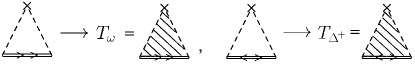
Figure 19: Replacement scheme from the AG level impurity scattering to self-consistent impurity treatment in BCS theory.

The above result can be easily extended to self-consistent impurity $T$-matrix calculations, by replacing the AG-level impurity scattering with the self-consistent impurity $T$-matrices, as shown in Fig. 19. The relationship between the regular and anomalous impurity $T$ matrices $T_{\omega}$ and $T_{\Delta^{\dagger}}$ are shown in Fig. 20. One can easily write down the corresponding equations, as follows.

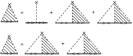
Figure 20: Relationship between impurity $T$ matrices $T_{\omega}$ and $T_{\Delta^{\dagger}}$ in BCS theory.

$$T_{\omega}=u+u\bar{\bar{G}}_{\omega}T_{\omega}-u\bar{\bar{F}}_{\omega}T_{\Delta^{\dagger}}\,,$$ (62a)

$$T_{\Delta^{\dagger}}=u\bar{\bar{F}}^{\dagger}_{\omega}T_{\omega}+u\bar{\bar{G}}_{-\omega}T_{\Delta^{\dagger}}\,.$$ (62b)

Finally, one has

$$T_{\omega}=\frac{u(1-u\bar{\bar{G}}_{-\omega})}{\left(1-u\bar{\bar{G}}_{\omega}\right)\left(1-u\bar{\bar{G}}_{-\omega}\right)+u^{2}\bar{\bar{F}}_{\omega}\bar{\bar{F}}^{\dagger}_{\omega}}\,,$$ (63a)

$$T_{\Delta^{\dagger}}(\omega)=\frac{u^{2}\bar{\bar{F}}^{\dagger}_{\omega}}{\left(1-u\bar{\bar{G}}_{\omega}\right)\left(1-u\bar{\bar{G}}_{-\omega}\right)+u^{2}\bar{\bar{F}}_{\omega}\bar{\bar{F}}^{\dagger}_{\omega}}\,,$$ (63b)

where $\bar{\bar{G}}=\sum_{\mathbf{k}}G(K)$, $\bar{\bar{F}}^{\dagger}=\sum_{\mathbf{k}}F^{\dagger}(K)$, and similarly for their complex conjugate. Note these two equations are formally identical to Eqs. (37a) and (37c), except that the current $T_{\Delta^{\dagger}}$ contains the factor $\Delta$ already.

Now with the new definition $i\tilde{\omega}=i\omega-\Sigma_{\omega}$, $i\tilde{\underline{\omega}}=-i\omega-\Sigma_{-\omega}$, $\tilde{\Delta}_{\bf k}=\Delta_{\bf k}+\Sigma_{\Delta}$, and $\tilde{\Delta}^{*}_{\bf k}=\Delta_{\bf k}^{*}+\Sigma_{\Delta}^{*}$, as well as $\Sigma_{\omega}=n_{i}T_{\omega}$ and $\Sigma^{*}_{\Delta}=n_{i}T_{\Delta^{\dagger}}$, Eqs. (61b) for $G$ and $F$ remain valid.

References

- Anderson (1987) P. W. Anderson, Science 235, 1196 (1987).
- Chakravarty et al. (2001) S. Chakravarty, R. B. Laughlin, D. K. Morr, and C. Nayak, Phys. Rev. B 63, 094503 (2001).
- Demler et al. (2001) E. Demler, S. Sachdev, and Z. Y, Phys. Rev. Lett. 87, 067202 (2001).
- Emery and Kivelson (1995) V. J. Emery and S. A. Kivelson, Nature 374, 434 (1995).
- Randeria (1995) M. Randeria, in Bose Einstein Condensation, edited by A. Griffin, D. Snoke, and S. Stringari (Cambridge Univ. Press, Cambridge, 1995), pp. 355–92.
- Maly et al. (1999a) J. Maly, B. Jankó, and K. Levin, Physica C 321, 113 (1999a).
- Maly et al. (1999b) J. Maly, B. Janko, and K. Levin, Phys. Rev. B 59, 1354 (1999b).
- Janko et al. (1997) B. Janko, J. Maly, and K. Levin, Phys. Rev. B 56, R11407 (1997).
- Chen et al. (1998) Q. J. Chen, I. Kosztin, B. Janko, and K. Levin, Phys. Rev. Lett. 81, 4708 (1998).
- Kosztin et al. (1998) I. Kosztin, Q. J. Chen, B. Janko, and K. Levin, Phys. Rev. B 58, R5936 (1998).
- Chen et al. (1999) Q. J. Chen, I. Kosztin, B. Janko, and K. Levin, Phys. Rev. B 59, 7083 (1999).
- Chen et al. (2000a) Q. J. Chen, I. Kosztin, and K. Levin, Phys. Rev. Lett. 85, 2801 (2000a).
- Kruis et al. (2001) H. V. Kruis, I. Martin, and A. V. Balatsky, Phys. Rev. B 64, 054501 (2001).
- Hirschfeld and Vollhardt (1986) P. Hirschfeld and P. Vollhardt, D Wölfle, Solid State Commun. 59, 111 (1986).
- Hirschfeld et al. (1988) P. J. Hirschfeld, P. Wölfle, and D. Einzel, Phys. Rev. B 37, 83 (1988).
- Hirschfeld and Goldenfeld (1993) P. J. Hirschfeld and N. Goldenfeld, Phys. Rev. B 48, 4219 (1993).
- Senthil and Fisher (1999) T. Senthil and M. P. A. Fisher, Phys. Rev. B 60, 6893 (1999).
- Pépin and Lee (2001) C. Pépin and P. A. Lee, Phys. Rev. B 63, 054502 (2001).
- Ziegler et al. (1998) K. Ziegler, M. H. Hettler, and P. J. Hirschfeld, Phys. Rev. B 57, 10 825 (1998).
- Atkinson et al. (2000a) W. A. Atkinson, P. J. Hirschfeld, A. H. MacDonald, and K. Ziegler, Phys. Rev. Lett. 85, 3926 (2000a).
- Kadanoff and Martin (1961) L. P. Kadanoff and P. C. Martin, Phys. Rev. 124, 670 (1961).
- Abrikosov and Gor’kov (1959) A. A. Abrikosov and L. P. Gor’kov, Sov. Phys. JETP 35, 1090 (1959), Zh. Eksp. Teor. Fiz. 35, 1558-1571 (1958).
- Abrikosov and Gor’kov (1960) A. A. Abrikosov and L. P. Gor’kov, Sov. Phys. JETP 10, 593 (1960), Zh. Eksp. Teor. Fiz. 39, 1781 (1960).
- (24) A. A. Abrikosov, L. P. Gor’kov, and I. E. Dzyaloshinski, Methods of quantum field theory in statistical physics (Prentice-Hall, Englewood Cliffs, N.J., 1963).
- Kosztin et al. (2000) I. Kosztin, Q. J. Chen, Y.-J. Kao, and K. Levin, Phys. Rev. B 61, 11 662 (2000).
- Ishida et al. (1993) K. Ishida, Y. Kitaoka, N. Ogata, T. Kamino, K. Asayama, J. R. Cooper, and N. Athanassopovlov, J. Phys. Soc. Jpn. 62, 2803 (1993).
- Fehrenbacher (1996) R. Fehrenbacher, Phys. Rev. Lett. 77, 1849 (1996).
- Bocquet et al. (2000) M. Bocquet, D. Serban, and M. R. Zirnbauer, Nucl. Phys. B 578, 628 (2000).
- Atkinson et al. (2000b) W. A. Atkinson, P. J. Hirschfeld, and A. H. MacDonald, Physica C 341, 1687 (2000b).
- Franz et al. (1997) M. Franz, C. Kallin, A. J. Berlinsky, and M. I. Salkola, Phys. Rev. B 56, 7882 (1997).
- Williams et al. (1995) G. V. M. Williams, J. L. Tallon, R. Meinhold, and A. Janossy, Phys. Rev. B 51, 16 503 (1995).
- Williams et al. (1998) G. V. M. Williams, E. M. Haines, and J. L. Tallon, Phys. Rev. B 57, 146 (1998).
- MacFarlane et al. (2000) W. A. MacFarlane, J. Bobroff, H. Alloul, P. Mendels, N. Blanchard, G. Collin, and J. F. Marucco, Phys. Rev. Lett. 85, 1108 (2000).
- Bobroff et al. (1999) J. Bobroff, W. A. MacFarlane, H. Alloul, P. Mendels, N. Blanchard, G. Collin, and J. F. Marucco, Phys. Rev. Lett. 83, 4381 (1999).
- Hanaki et al. (2001) Y. Hanaki, Y. Ando, S. Ono, and J. Takeya, Phys. Rev. B 64, 172514 (2001).
- Chen et al. (2000b) Q. J. Chen, I. Kosztin, and K. Levin, Physica C 341, 149 (2000b).
- Carrington et al. (1999) A. Carrington, I. J. Bonalde, R. Prozorov, R. W. Giannetta, A. M. Kini, J. Schlueter, H. H. Wang, U. Geiser, and J. M. Williams, Phys. Rev. Lett. 83, 4172 (1999).
- Bernhard et al. (1996) C. Bernhard, J. L. Tallon, C. Bucci, R. De Renzi, G. Guidi, G. V. M. Williams, and C. Niedermayer, Phys. Rev. Lett. 77, 2304 (1996).
- (39) D. A. Bonn, S. Kamal, A. Bonakdarpour, R. X. Liang, W. N. Hardy, C. C. Homes, D. N. Basov, and T. Timusk, Czech J. Phys. 46, suppl. 6, 3195 (1996).
- Chen et al. (2001) Q. J. Chen, K. Levin, and I. Kosztin, Phys. Rev. B 63, 184519 (2001).
- Anderson (1959) P. W. Anderson, J. Phys. Chem. Solids 11, 26 (1959).
- (42) L. P. Gor’kov, Pis’ma Zh. Eksp. Teor. Fiz. 40, 351 (1984). [Sov. Phys. JETP Lett. 40, 1155 (1985)].
- (43) Of course, when is too large, all pairs will be destroyed.