Critical Casimir Forces in Colloidal Suspensions

Abstract

Some time ago, Fisher and de Gennes pointed out that long-ranged correlations in a fluid close to its critical point $T_{c}$ cause distinct forces between immersed colloidal particles which can even lead to flocculation [C. R. Acad. Sc. Paris B 287, 207 (1978)]. Here we calculate such forces between pairs of spherical particles as function of both relevant thermodynamic variables, i.e., the reduced temperature $t=(T-T_{c})/T_{c}$ and the field $h$ conjugate to the order parameter. This provides the basis for specific predictions concerning the phase behavior of a suspension of colloidal particles in a near-critical solvent.

I Introduction

In 1978 Fisher and de Gennes [1] predicted that the confinement of critical fluctuations of the order parameter in a binary liquid mixture near its critical demixing point $T_{c}$ gives rise to long-ranged forces between immersed plates or particles. In particular, they pointed out that these long-ranged forces would eventually lead to the flocculation of colloidal particles which are dissolved in a near-critical binary liquid mixture [2]. A few years later, such a solvent-mediated flocculation was observed experimentally for silica spheres immersed in the binary liquid mixture of water and 2,6-lutidine [3, 4]. However, the precise interpretation of these experiments is still under debate; although fluctuation-induced forces as predicted by Fisher and de Gennes certainly play a major role, additional mechanisms, such as screening effects in the case of charged colloidal particles [3], may also contribute [5]. In the meantime additional experimental evidence for this kind of flocculation phenomena has emerged for other binary mixtures acting as solvents [6, 7, 8].

From a colloid physics perspective effective, solvent-mediated interactions between dissolved colloidal particles are of basic importance [9, 10, 11, 12]. The richness of the physical properties of these systems is mainly based on the possibility to tune these effective interactions over wide ranges of strength and form of the interaction potential. Traditionally, this tuning is accomplished by changing the chemical composition of the solvent by adding salt, polymers, or other components [9, 10, 11, 12]. Compared with such modifications, changes of the temperature or pressure typically result only in minor changes of the effective interactions. On the other hand, however, effective interactions generated by bringing solvents close to a phase transition of their own are extremely sensitive to such changes. In this broader context, flocculation of colloidal particles induced by critical fluctuations near a second-order phase transition of the solvent as predicted by Fisher and de Gennes [1, 2] provided the first instance in which effective interactions are tuned by changing the physical conditions rather than the chemical composition of the solvent. Later on, this idea has been extended to first-order transitions of the solvent, for which wetting transitions can occur which give rise to wetting films of the preferred phase coating the colloidal particles [13, 14, 15, 16]. In the meantime the study of effective interactions between dissolved particles generated by changing the physical conditions of the solvent, and the resulting phase behavior of the colloidal suspension, has emerged as one of the main fields of research in colloid physics [14].

The physical origin of the force predicted by Fisher and de Gennes is analogous to the Casimir force between conducting plates, which arises due to the confinement of quantum mechanical vacuum fluctuations of the electromagnetic field [17, 18, 19]. (Related phenomena occur in string theory [20], liquid crystals (see, e.g., ref. [21]), and microemulsions [22]. However, in contrast to the present so-called “critical Casimir effect”, in liquid crystals the director-fluctuation induced forces are notoriously difficult to separate from the background of dispersion forces due to the absence of a singular temperature dependence [23].) In recent years this “critical Casimir effect” has attracted increasing theoretical [24, 25, 26, 27, 28] and experimental [5, 29, 30] interest. In this case the fluctuations are provided by the critical order parameter fluctuations of a bona fide second-order phase transition in the corresponding bulk sample. For He⁴ wetting films close to the superfluid phase transition the theoretical predictions [25] for critical Casimir forces between parallel surfaces exhibiting Dirichlet boundary conditions have been confirmed quantitatively [30]. These quantum fluids offer the opportunity to study critical Casimir forces in the absence of surface fields, i.e., the purely fluctuation induced forces.

In a classical binary liquid mixture near its critical demixing point, the order parameter is a suitable concentration difference between the two species forming the liquid. In this case the inevitable preference of confining boundaries for one of the two species results in the presence of effective surface fields leading to nonvanishing order parameter profiles even at $T\geq T_{c}$ [31]. (This is the case discussed by Fisher and de Gennes [1, 2].) These so-called “critical adsorption” profiles become particularly long-ranged due to the correlation effects induced by the critical fluctuations of the order parameter of the solvent. In the case of a planar wall, critical adsorption has been studied in much detail [32, 33, 34, 35, 36, 37, 38, 39]. Asymptotically close to the critical point $T_{c}$ it is characterized by a surface field which is infinitely large so that the order parameter profile actually diverges upon approaching the wall up to atomic distances. Later on, critical adsorption on curved surfaces of single spherical and rodlike colloidal particles has been studied, where it turns out, in particular, that critical adsorption on a microscopically thin “needle” represents a distinct universality class of its own [40, 41]. Critical adsorption on the rough interface between the critical fluid and its noncritical vapor occurring at the critical end point of the binary liquid mixture has been addressed as well [42]; likewise the effect of quenched surface modulations and roughness [43]. The interference of critical adsorption on neighboring spheres gives rise to the critical Casimir forces which have been argued to contribute to the occurrence of flocculation near $T_{c}$ [2, 44, 45, 46]. However, a quantitative understanding of these phenomena requires the knowledge of the critical adsorption profiles near the colloidal particles and the resulting effective free energy of interaction in the whole vicinity of the critical point, i.e., as function of both the reduced temperature $t=(T-T_{c})/T_{c}$ and the bulk field $h$ conjugate to the order parameter. So far, this ambitious goal has not yet been accomplished. Instead, the introduction of the additional complication of a surface curvature has limited the knowledge of the corresponding critical adsorption so far to the case of spheres for the particular thermodynamic state $(t,h)=(0,0)$ of the solvent [44, 47, 48, 49].

In a previous work [46], at least the temperature dependence of the critical Casimir force between a sphere and a planar container wall has been discussed. It turns out that the force becomes maximal not at but above $T_{c\,}$. In ref. [46] also the force $F$ between a pair of spheres of radius $R$ at distance $D+2\,R$ between their centers (see Fig. 1) has been briefly analyzed. Close to the critical demixing point, this force separates into a regular background contribution and a singular contribution $F^{\pm}_{\text{sing}}$ of universal character, which is attractive if the same of the two coexisting bulk phases is enriched near both spheres. The results for $F^{\pm}_{\text{sing}}$ can be cast into the form

$$F^{\pm}_{\text{sing}}(D,R;t,h)\,=\,\frac{k_{B}T_{c}}{R}\,K_{\pm}\left(\Delta=\frac{D}{R}\,,\,\Theta_{\pm}=\frac{D}{\xi_{\pm}}\,,\,\Xi=\text{sgn}(h)\,\frac{D}{l_{H}}\right)\,\,,$$ (1)

where $\xi=\xi_{\pm}$ is the true correlation length governing the exponential decay of the order parameter correlation function in the bulk for $t=(T-T_{c})/T_{c}\gtrless 0$ at $h=0$; $l_{H}$ is the correlation length governing the exponential decay of the order parameter correlation function for $h\to 0$ at $t=0$. $K_{\pm}$ are universal scaling functions. Note that surface fields $h_{1}$ break the symmetry $h\,\to\,-h$, i.e., $F^{\pm}_{\text{sing}}$ depends on the sign of $\Xi$. Here and in the following we consider only the fixed point value $h_{1}\to+\infty$.

The aim of this work is to study the critical Casimir force between two spherical colloidal particles as function of both relevant thermodynamic variables $t$ and $h$. Figure 2 shows the schematic phase diagram of the solvent, e.g., a binary liquid mixture. Different thermodynamic paths are indicated along which the dependence of the force on $t$ and $h$ is studied.

The remainder of this work is organized as follows: In Sec. II we define the field-theoretic model used to describe the near-critical solvent. In Sec. III the numerical calculation of the adsorption profiles in mean-field approximation is discussed. In Sec. IV we present the results for the force between two spherical particles and compare them with the limiting cases of small and large particle radii. The discussion of the results for two parallel plates, which inter alia are relevant for a pair of spheres via the Derjaguin approximation, is left to Sec. V. Finally, in Sec. VI, we summarize and discuss our results with regards to the phase behavior of a suspension of colloidal particles in a near-critical fluid.

II Field-theoretic model

Near criticality the behavior of the system is governed by fluctuations of the order parameter $\Phi$ on a large length scale such that the emerging universal properties are independent of microscopic details. A coarse-graining procedure leads to the continuum description in terms of the Ginzburg-Landau Hamiltonian [32, 33, 50]

$${\cal H}\{{\Phi}({\bf r})\}=\int\limits_{V}d^{d}r\,\Big{\{}\frac{1}{2}[\nabla{\Phi}({\bf r})]^{2}\,+\,\frac{\tau}{2}\,{\Phi}^{2}({\bf r})\,+\,\frac{u}{24}\,{\Phi}^{4}({\bf r})\,-\,{h}\,{\Phi}({\bf r})\Big{\}}\,$$ (2)

of an order parameter field ${\Phi}({\bf r})$ in the bulk of volume $V$. For the liquids considered here ${\Phi}({\bf r})$ is a scalar field. The Hamiltonian determines the statistical weight $\exp[-{\cal H}\{{\Phi}({\bf r})\}]$ of the configuration $\{{\Phi}({\bf r})\}$. The external bulk field ${h}({\bf r})$ is conjugate to the order parameter and breaks its symmetry. The temperature dependence enters via

$$\tau\sim t=\frac{T-T_{c}}{T_{c}}\quad.$$ (3)

The partition function of the system is given by

$${\cal Z}(\tau,h;u)=\int{\cal D}\{{\Phi}\}\,\exp[-{\cal H}\{{\Phi}({\bf r})\}]\quad,$$ (4)

where ${\cal D}\{{\Phi}\}$ denotes an appropiately defined functional integration [33]. The corresponding singular part of the free energy reads

$${\cal F}_{\rm sing}(\tau,h;u)=-k_{B}\,T_{c}\,\ln{\cal Z}(\tau,h;u)\;.$$ (5)

The coarse-graining procedure leading to a continuum model from a given lattice model can be generalized to systems with surfaces resulting in the Hamiltonian [32, 33]

$${\cal H}\{{\Phi}({\bf r})\}\, = \,\int\limits_{V}d^{d}r\,\Big{\{}\frac{1}{2}[\nabla{\Phi}({\bf r})]^{2}\,+\,\frac{\tau}{2}\,{\Phi}^{2}({\bf r})\,+\,\frac{u}{24}\,{\Phi}^{4}({\bf r})\,-\,{h}\,{\Phi}({\bf r})\Big{\}}$$ (6)

$$+ \,\int\limits_{S}dS\,\Big{\{}\frac{c}{2}\,{\Phi}^{2}({\bf r}_{S})\,-\,{h}_{1}\,{\Phi}({\bf r}_{S})\Big{\}}\;.$$ (7)

The first integral runs over the volume $V$ available for the critical medium, which is bounded by the surface(s) $S=\partial\,V$. Apart from the restricted space integration, the first integral in Eq. (7) has the same form as the Hamiltonian (2) for bulk systems disregarding surfaces. The second integral in Eq. (7) represents a surface contribution in which the integral runs over the boundary surface $S=\partial\,V$; $c$ is related to the strength of the coupling of critical degrees of freedom near the surface and $h_{1}$ is the surface analogue of the bulk field $h$ [32, 33].

The systematic treatment of the critical fluctuations as implied by Eq. (4) and a justification of the form of ${\cal H}\{{\Phi}({\bf r})\}$ is provided by the field-theoretic renormalization group framework [33]. The basic idea is to consider the physical system on larger and larger length scales and to single out those quantities which eventually remain unchanged under the repeated action of such scale transformations. Such quantities tend to their fixed point values right at the critical point [50]. For bulk systems, there remain only two relevant adjustable parameters, corresponding to $\tau$ and $h$. The surface generates a subdivision of a given bulk universality class into different surface universality classes characterized by different fixed point values for $c$ and $h_{1}$. For $h_{1}=0$ the corresponding leading singular behaviors are determined by the fixed-point values $c=+\infty$ for the ordinary transition (O), $c=0$ for the special or surface-bulk transition, and $c=-\infty$ for the extraordinary or normal transition (E) [32, 33]. For the O and E transitions only $\tau$, $h$, and $h_{1}$ remain as relevant variables. The three cases above were originally studied for magnetic systems. For liquids, however, E is the generic case and therefore it is called the normal transition. The case $h_{1}=\infty$ with $c$ arbitrary corresponds to critical adsorption, but the leading singular behavior is the same as for the E transition [36].

Neglecting fluctuations the Ginzburg-Landau Hamiltonian ${\cal H}\{\Phi({\bf r})\}$ itself represents a free energy functional which upon minimization with respect to $\Phi({\bf r})$ yields the Euler-Lagrange equations for order parameter profiles and correlation functions. The minimization is equivalent to the mean-field description of the system,

$$\left.\frac{\delta\,{\cal H}\{{\Phi}({\bf r})\}}{\delta\,{\Phi}({\bf r})}\right|_{{\Phi}=\langle{\Phi}\rangle}=0\;,$$ (8)

where the fluctuating order parameter ${\Phi}$ is replaced by its mean value $\langle{\Phi}\rangle$. The universal critical behavior is captured correctly by mean-field theory if the space dimension $d$ exceeds the upper critical dimension $d_{\text{uc}}=4$.

Because of the relative complexity of the geometry considered here (see Fig. 1), it is not possible to carry out the complete renormalization procedure in closed form. Instead, available knowledge for bulk systems in $d=3$ is used in combination with the mean-field solution for the geometry considered here in order to estimate universal quantities in $d=3$. An alternative way to overcome mean-field theory is followed within the concept of the Local Functional Theory developed in refs. [51, 52, 53, 54], in which the free energy is described by a functional depending locally on the order parameter and its derivative. With mean-field theory as a special case, it takes into account available knowledge in $d=3$, such as the correct values for the critical exponents.

III Order parameter profiles

In this Section we describe some technical aspects of the tools and numerical methods used for obtaining the mean-field results, i.e., the determination of the order parameter profiles at the critical point, the short distance expansion of the profile close to a surface, the minimization procedure to determine the profiles away from the critical point, and the calculation of the force between the particles based on the stress tensor.

Minimization in Eq. (8) leads to the differential equation

$$-\Delta\,m+\tau\,m+m^{3}-H=0\;,$$ (9)

where the coupling constant $u$ is absorbed in the order parameter and in the bulk magnetic field,

$$m=\sqrt{\frac{u}{6}}\,\langle{\Phi}\rangle\>,\;H=\sqrt{\frac{u}{6}}\,h\;.$$ (10)

Note that we are interested in an estimate of the order parameter profile $m$ in $d=3$ where, at the fixed point, $u$ is a positive number. For $d\nearrow 4$ the mean-field solution is exact, but the fixed point value of the coupling constant $u$ vanishes in this limit.

The surface integrals in Eq. (7) lead to a boundary condition for the order parameter at the surfaces of the spherical particles. At the critical adsorption fixed point this boundary condition is given by

$$\Phi_{S}=\infty\;.$$ (11)

A Order parameter profiles at criticality

While our main interest is the dependence of the Casimir force on $t$ and $h$, the knowledge of the order parameter profile at the critical point, i.e., for $(t,h)=(0,0)$, is a useful starting point. In ref. [48] this latter profile is given for a critical system confined to a spherical shell between two concentric spheres with radii $R_{\pm}$ at which the order parameter diverges. In terms of elliptic functions it reads

$$m(r)=\frac{\displaystyle\sqrt{\frac{1-k^{2}}{k^{2}-\frac{1}{2}}}}{\displaystyle r\,\mbox{cn}\left(\sqrt{\frac{1}{2k^{2}-1}}\>\ln\left(\frac{r}{R_{0}}\right)\right)}\;,$$ (12)

where $r$ is the radial distance from the common center of the spheres and $k$ is the module of the elliptic function cn [55]. The module $k$ must be adjusted such that the profile diverges at the given radii $R_{\pm}$ leading to the following implicit equation for $k$:

$$\frac{R_{\pm}}{R_{0}}=\left(\frac{R_{+}}{R_{-}}\right)^{\pm\frac{1}{2}}=\,\exp{\left(\pm{\sqrt{2k^{2}-1}}\,{K(k)}\right)}\;,$$ (13)

where $R_{0}=\sqrt{R_{+}\,R_{-}}$ is the geometric mean of the radii and $K$ is the complete elliptic integral of the first kind.

In ref. [44] it is outlined how the results for concentric spheres can be used for different geometries via a conformal transformation of the coordinates,

$$\frac{{\bf r}^{\,\prime}}{|{\bf r}^{\,\prime}|^{2}}=\frac{{\bf r}+{\bf R}}{|{\bf r}+{\bf R}|^{2}}-\frac{{\bf R}}{2\,|{\bf R}|^{2}}\;,$$ (14)

where ${\bf r}^{\,\prime}$ and ${\bf r}$ are the new and the old coordinates, respectively, and ${\bf R}$ defines the symmetry axis and the eventual shape of the new geometry. For $|{\bf R}|=R_{0}$ the two concentric spheres with radii $R_{\pm}$ are mapped onto two spheres of equal size which is the generic case we are interested in. For $|{\bf R}|=R_{+}$ the two concentric spheres are mapped onto a single spherical particle in front of a planar wall for which results were obtained in ref. [46].

Under the conformal transformation (14), each local scaling field is multiplied by a scale factor

$$b({\bf r}^{\,\prime})=1+\frac{{\bf R}\cdot{\bf r}^{\,\prime}}{|{\bf R}|^{2}}+\frac{|{\bf r}^{\,\prime}|^{2}}{4\,|{\bf R}|^{2}}\;,$$ (15)

which is raised to the power of the scaling dimension of this scaling field. In mean-field approximation and $d=4$, the scaling dimension of the order parameter $\Phi$ is $1$, which implies for the order parameter profile

$$m({\bf r}^{\,\prime})=b({\bf r}^{\,\prime})^{-1}\,m_{\text{conc}}(|{\bf r}({\bf r}^{\,\prime})|)\;,$$ (16)

where $m_{\text{conc}}(|{\bf r}|)$ is the profile in the concentric geometry given by Eq. (12).

Let $D$ denote the surface-to-surface distance between the two spheres and $R$ their common radius; then the corresponding radii $R_{\pm}$ in the concentric geometry are given by

$$R_{\pm}=\frac{D}{4}\,A\left(\frac{A+1}{A-1}\right)^{\pm 1}$$ (17)

with the abbreviation

$$A=\sqrt{1+4\,\frac{R}{D}}\;.$$ (18)

Putting the pieces together, Eqs. (10)-(17) yield the order parameter profile in the geometry of two spherical particles with radius $R$ a distance $D$ apart from each other right at the critical point $(t,h)=(0,0)$.

B Short distance expansion

In the following we describe the methods for obtaining results off criticality, i.e., for $t\gtrless 0$ and $h\neq 0$, i.e., $\tau\gtrless 0$ and $H\neq 0$. Equation (9) will then yield a different profile $m({\bf r}^{\,\prime})$. However, the profile at the critical point serves as a suitable starting point for the minimization procedure (8). Close to the surfaces it is even possible to calculate the deviation of the order parameter from the profile at the critical point analytically. In this context the so-called short distance expansion turns out to be useful, and has been carried out for $\tau\gtrless 0$ in ref. [40]. With $H\neq 0$ in addition, it reads:

$$m(s\to 0;R,\tau,H) = \frac{\sqrt{2}}{s}-\frac{\sqrt{2}}{6}\frac{d-1}{R}$$ (19)

$$+ \frac{\sqrt{2}}{6}\,s\Big{\{}-\,\tau+\Big{[}\frac{5}{6}\,\frac{(d-1)^{2}}{R^{2}}\,-\,\frac{(d-1)(d-2)}{R^{2}}\Big{]}\Big{\}}$$ (20)

$$+ \frac{\sqrt{2}}{4}\,s^{2}\Big{(}\frac{H}{\sqrt{2}}-\frac{d-1}{3\,R}\,\tau-\frac{4d^{3}-39d^{2}+120d-85}{54\,R^{3}}\Big{)}$$ (21)

$$+ {\cal O}(s^{3})\;,$$ (22)

where $s$ is the radial distance from the surface of a sphere with radius $R$. The difference $\delta m=m(s\to 0;R,\tau,H)-m(s\to 0;R,\tau=0,H=0)$ gives the deviation from the profile at the critical point close to the surfaces. While the profile itself diverges at the surfaces, the deviation $\delta m$ vanishes with the radial distance $s$ as

$$\delta m(s\to 0;R,\tau,H)=-\frac{\sqrt{2}}{6}\,\tau\,s+\frac{1}{4}\left(H-\frac{\sqrt{2}}{3}\frac{d-1}{R}\,\tau\right)\,s^{2}+\ldots\;,$$ (23)

where the bulk field $H$ and the radius $R$ of the spherical particles appear only in ${\cal O}(s^{2})$ and higher order. Equation (19) is only valid for small $s$ since the presence of the second particle is neglected. Corrections to Eqs. (19) and (23), however, are of order ${\cal O}(s^{3})$ as derived for the case of parallel plates, where they are called distant wall corrections [1, 56].

C Numerical solution for the complete profiles off criticality

So far we have provided results for the order parameter profile at the critical point for the two sphere geometry [Eq. (16)] and off criticality but close to the surface of a single sphere [Eq. (19)]. In order to obtain the complete order parameter profile away from the critical point for the geometry consisting of two spheres with equal size (see Fig. 1) additional, numerical effort is required.

Upon discretization the order parameter profile $m({\bf r}^{\,\prime};D,R;\tau,H)$ in the two sphere geometry (Fig. 1) is described by a set of parameter values $a_{ij}$ where $i$ and $j$ indicate the dependence on the two independent spatial variables required for the present cylindrical symmetry around the axis between the two centers of the spheres [see, c.f., Eq. (26)]:

$$m({\bf r}^{\,\prime};D,R;\tau,H)=m(\{a_{ij}\})\;.$$ (24)

Within mean-field theory ${\cal H}(\{a_{i,j}\})$ has to be minimized with respect to $\{a_{ij}\}$ for given $D$, $R$, $\tau$, and $H$. To this end we apply the method of steepest descent [57],

$$a_{ij}^{\,(n+1)}=a_{ij}^{\,(n)}-\kappa\,\frac{\partial\,{\cal H}(\{a_{ij}\})}{\partial\,a_{ij}}\Bigg{|}_{\textstyle a_{ij}^{\,(n)}}\;,$$ (25)

where $\kappa$ is a positive number and $a_{ij}^{\,(n)}$ is the $n$-th iteration of the parameter $a_{ij}$.

It is known that in general the method of steepest descent converges slowly. Nevertheless in the present case it is found to be useful since the dependence on the choice of the initial set of parameters $\{a_{ij}^{\,(0)}\}$ is weak. In fact, it turns out that the profile at the critical point is a rather useful starting profile. The convergence also depends on the value of $\kappa$: if it is chosen too large, the convergence breaks down, if it is chosen too small, the convergence becomes too slow. As we will discuss later, one advantage of the present minimization method is that the explicit evaluation of the Hamiltonian $\cal H$ is not necessary, since only the gradient $\frac{\partial\,{\cal H}(\{a_{ij}\})}{\partial\,a_{ij}}$ is needed, which can be obtained independently. In order to keep this advantage, iterative methods to determine the best choice for the value of $\kappa$, which explicitly need the value of the functional that is to be minimized, are not applied. Nonetheless the best choice of $\kappa$ is the largest value for which the minimization still proceeds.

In particular, we use the parametrization

$$m({\bf r}^{\,\prime}_{ij};D,R;\tau,H)=m({\bf r}^{\,\prime}_{ij};D,R;0,0)+a_{ij}\;,$$ (26)

where ${\bf r}^{\,\prime}_{ij}$ denotes discretized spatial positions in the two sphere geometry, $m({\bf r}^{\,\prime}_{ij};D,R;0,0)$ is the value of the order parameter profile for $(\tau,H)=(0,0)$ at those positions, according to Eq. (16), and $a_{ij}$ denotes the deviation from this value at the position ${\bf r}^{\,\prime}_{ij}$ used in the minimization procedure (25). Thus starting the procedure with the profile for $(\tau,H)=(0,0)$ implies the choice

$$a_{ij}^{(0)}=0\;,\quad\forall\;i,j\,.$$ (27)

In addition, Eq. (23) provides the behavior of the $a_{ij}$ for ${\bf r}^{\,\prime}_{ij}$ close to the surface, i.e., $a_{ij}^{(n)}=0$ for all $n$ if ${\bf r}^{\,\prime}_{ij}={\bf r}^{\,\prime}_{S}$. From Eq. (23) even the slope of a function $f(s)$ used for interpolating the $a_{ij}$ as function of the radial distance $s$ from the surface of the sphere is known for $s\to 0$.

The cylindrical symmetry of the problem allows one to consider the planar geometry depicted in Fig. 1. Instead of discretizing the space by a square lattice we use a lattice which takes into account that there are areas with strong changes in the order parameter $m$, i.e., close to the surfaces, and areas with weak changes, i.e., far away from the spheres. In those areas with weak changes less lattice points are needed. For this purpose we use what we call the conformal lattice. The idea is to use the conformal mapping (14) in order to create this lattice from that one for the case of concentric spheres. In analogy to electrostatics the field lines and the lines of equal potential of a system with two concentric spheres forming the two electrodes of a capacitor are mapped onto the two sphere geometry such that the new lines are the field lines and the lines of equal potential of a system with two charged spheres. The intersections of these lines form the lattice sites of the conformal lattice. The advantage of this lattice is that the field lines approach the spheres perpendicularly to their surface, which allows one to use the short distance behavior [Eqs. (19) and (23)] as a boundary condition for the $a_{ij}$. Figure 3 shows the conformal lattice for the geometry of two spheres. In principle, it would be possible to use only one half of this lattice, since this system is symmetric with respect to the vertical midplane. However, this reduction leaves one with a disadvantage. The value of the order parameter at this midplane wall is not known, and thus it must be determined within the minimization process. The minimization turns out to be inefficient then. Therefore for the two sphere geometry we resort to the full conformal lattice enclosing both spheres as shown in Fig. 3.

The Hamiltonian $\cal H$ [Eq. (7)] is given by

$${\cal H}=\frac{6}{u}\int\limits_{V}dV{\cal L}(m)+\frac{6}{u}\int\limits_{S}dS{\cal L}_{S}(m)\;,$$ (28)

with

$${\cal L}(m)=\frac{1}{2}(\nabla m)^{2}+\frac{\tau}{2}m^{2}+\frac{1}{4}m^{4}-H\,m$$ (29)

and ${\cal L}_{S}(m)=\frac{c}{2}\,m^{2}-H_{1}\,m$ with $H_{1}=h_{1}\,\sqrt{u/6}$. Performing the functional derivative with respect to the order parameter $m$ leads, via partial integration, to

$$\frac{\delta\,{\cal H}\{m({\bf r})\}}{\delta\,m({\bf r})}=\frac{6}{u}\int_{V}\!dV\{-\Delta\,m+\tau\,m+m^{3}-H\}+\frac{6}{u}\int_{S}\!dS\,\{-\partial_{n}\,m+{\cal L}^{\prime}_{S}(m)\}\;,$$ (30)

where $\partial_{n}\,m$ is the derivative of the order parameter in direction of the surface normal. We note that the surface integral vanishes, if the boundary conditions [Eqs. (19) and (23)] are fulfilled. Equation (25) contains the derivative of the Hamiltonian ${\cal H}$ with respect to the parameters $a_{ij}$ which represent the order parameter $m$. With $m=m(a_{ij})=const$ in a small volume $\delta V({\bf r}^{\,\prime}_{ij})$ around the position ${\bf r}^{\,\prime}_{ij}$ the gradient in Eq. (25) is approximated by

$$\frac{\partial\,{\cal H}(\{a_{ij}\})}{\partial\,a_{ij}}=\frac{6}{u}\,{\delta V({\bf r}^{\,\prime})}\,\{-\Delta\,m+\tau\,m+m^{3}-H\}\Big{|}_{\displaystyle{\bf r}^{\,\prime}={\bf r}^{\,\prime}_{ij}}\quad.$$ (31)

Note that a constant prefactor in Eq. (31) can be absorbed by a rescaling of $\kappa$ in Eq. (25). If Eq. (9) holds, i.e., if the expression in curly brackets in Eq. (31) vanishes, Eq. (25) reduces to

$$a_{ij}^{\,(n+1)}=a_{ij}^{\,(n)}\;,$$ (32)

i.e., the minimization has led to a fixed point solution of the iteration.

For the minimization process the second derivatives of the order parameter profile are needed [see Eq. (31)]. Since the order parameter is calculated only at the discrete sites ${\bf r}^{\,\prime}_{ij}$, numerical differentiation must be applied. For a numerical derivative, in general, it is preferable to have the sites on an equidistant square lattice. However, it is also possible to deal with derivatives on the conformal lattice. To this end we have used the spline approximation [58] in order to interpolate between all the $a_{ij}$ on each of the lines of the conformal lattice (see Fig. 3). This approximation directly yields the second derivative of the order parameter at the lattice sites with respect to the variables parametrizing the lines. Under a conformal mapping angles are conserved, so that the lines in the conformal lattice intersect perpendicularly which allows one to translate the derivatives obtained from the spline approximation into derivatives with respect to the cylindrical coordinates ${\bf r}^{\,\prime}=(\rho,z)$.

D Stress tensor

With the tools now available to determine the order parameter profile in the two sphere geometry the next step is to calculate the effective forces between the two spheres. The straightforward way to determine such forces is to calculate the free energy $\displaystyle-k_{B}T\,\ln{\cal Z}$ as function of the distance $D$ between the spheres, and then to estimate the derivative with respect to the distance by considering finite differences. However, the total value of the free energy is expected to be large as compared with the differences, and thus one has to deal numerically with differences between large numbers, which causes high inaccuracies. Therefore we resort to an alternative method, in which the force is calculated directly using the so-called stress tensor ${T}_{\mu\nu}$, which is defined by the linear response

$$\delta{\cal H}=\int_{V}d^{d}r\>\frac{\partial\,b_{\mu}}{\partial x_{\nu}}\>{T}_{\mu\nu}({\bf r})\;,$$ (33)

where ${\bf b}$ is a non-conformal coordinate transformation, $\mu$ and $\nu$ index the spatial coordinates, and $\delta{\cal H}$ is the corresponding energy shift. With the Lagrangian ${\cal L}(m)$ in Eq. (29) it reads [44, 46, 59]

$${T}_{\mu\nu}=\frac{6}{u}\left[\frac{\partial{\cal L}}{\partial(\partial_{\nu}m)}\partial_{\mu}m-\delta_{\mu\nu}{\cal L}\right]\;.$$ (34)

The knowledge of the stress tensor on any infinitely extended surface which separates the two spheres from one another, or likewise on any closed, finite surface which contains only one of the spheres, allows one to calculate the force between the spheres. This is illustrated in terms of the spherical volume $V_{S}$ with radius $\widetilde{R}$ containing the right sphere in Fig. 4. Using the coordinate transformation

$$b_{z} = \alpha\,,\;\forall\,{\bf r}\in V_{S}$$ (35)

$$= 0\,,\;\forall\,{\bf r}\not\in V_{S}$$ (36)

$$b_{\nu\neq z} = 0\;,$$ (37)

the volume $V_{S}$ is shifted in $z$-direction by the amount $\alpha$. The derivative $\frac{\partial\,b_{\mu}}{\partial x_{\nu}}$ then leads to a delta function such that the integral over the whole volume $V$ reduces to an integral over the boundary of $V_{S}$. In this case the force $F_{\text{sing}}=\frac{k_{B}\,T_{c}}{R}\,K$ with the universal scaling function $K$ [see Eq. (1)] is given by

$$-\frac{\displaystyle\partial\,\delta{\cal H}}{\partial\alpha} = -\frac{\displaystyle\partial}{\partial\alpha}\int_{V}d^{d}r\>\frac{\displaystyle\partial b_{\mu}}{\partial x_{\nu}}\>T_{\mu\nu}$$ (38)

$$= -\int_{\partial V_{S}}d\Omega\;n_{\nu}\>T_{z\nu}$$ (39)

$$= -4\pi\widetilde{R}^{3}\int^{\pi}_{0}d\varphi\sin^{2}\varphi\,[T_{zz}(\widetilde{R},\varphi)\,\cos\varphi+T_{z\rho}(\widetilde{R},\varphi)\,\sin\varphi]\quad,$$ (40)

where ${\bf n}$ is the unit vector perpendicular to the boundary $\partial V_{S}$. The quantities used in the parametrization in Eq. (39) are sketched in Fig. 4.

In the geometry with cylindrical symmetry [$m=m(\rho,z)$] considered here, Eq. (34) leads to

$$T_{zz}=\frac{1}{u}\left[3\left(\frac{\partial m}{\partial z}\right)^{2}+4\frac{m}{\rho}\frac{\partial m}{\partial\rho}+2m\frac{{\partial}^{2}m}{{\partial\rho}^{2}}-\left(\frac{\partial m}{\partial\rho}\right)^{2}-3\tau m^{2}-\frac{3}{2}m^{4}\right]$$ (41)

and

$$T_{z\rho}=\frac{1}{u}\left[4\left(\frac{\partial m}{\partial z}\right)\left(\frac{\partial m}{\partial\rho}\right)-2m\frac{{\partial}^{2}m}{{\partial\rho}{\partial z}}\right]\;,$$ (42)

where the so-called improvement term $-\frac{1}{u}(\nabla_{\mu}\nabla_{\nu}m^{2}-\delta_{\mu\nu}\Delta m^{2})$ has been added [59].

In our calculation, we choose $V_{S}$ as indicated in Fig. 3, determine the stress tensor at the lattice points, and use spline interpolations between them. Note that the possibility of choosing different spherical surfaces enclosing one of the spheres, which via Eq. (39) should all result in the same force $F_{\text{sing}}$, provides a valuable and sensitive check for both the validity and the accuracy of the numerical results.

IV Results for the two-particle interaction

The goal of this work is to provide a major step towards the understanding of aggregation of colloidal particles dissolved in a binary liquid mixture close to criticality. In the previous section we explained the various methods for obtaining the critical Casimir force between two spherical particles of equal size. The results are presented in this section.

The aggregation phenomenon is driven by the dependences on the temperature $t=(T-T_{c})/T_{c}$ and on the bulk composition $c_{A}$ of the solvent. While the former is related to the temperature parameter $\tau$ the latter is related to the bulk field $H$. Thus also the Casimir force between two particles must be determined as a function of those two parameters. We present results for the scaling function $K_{\pm}(\Delta=\frac{D}{R},\Theta_{\pm}=\frac{D}{\xi_{\pm}},\Xi=\text{sgn}(h)\,\frac{D}{l_{H}})$ which is related to the force $F^{\pm}_{\rm sing}$ between the particles via Eq. (1). The correlation length $\xi_{\pm}$ for $H=0$ depends on the temperature $T$ as [see also Eq. (3)]

$$\xi_{\pm}=\xi^{\pm}_{0}\,|t|^{-\nu}=\left\{\begin{array}[]{r@{\quad}l}\displaystyle{\tau^{\,-1/2}\,\,\,\,,}&{\tau>0}\\ \displaystyle{|2\,\tau|^{\,-1/2}\,\,\,,}&\tau<0\end{array}\right.\;,\quad H=0\;,$$ (43)

with $\nu=\frac{1}{2}$ within mean-field theory while the correlation length $l_{H}$ at $T_{c}$ depends on the bulk field $H$ as

$$l_{H}=l_{0}\,\left|\frac{c_{A}-c_{A,c}}{c_{A,c}}\right|^{-\nu/\beta}=\frac{1}{\sqrt{3}}\,{|H|}^{\,-{1}/{3}}\;,\quad\tau=0\;,$$ (44)

where $\nu/\beta=1$ within mean-field theory; $\xi^{\pm}_{0}$ and $l_{0}$ are nonuniversal amplitudes. The first parts of Eqs. (43) and (44) hold in general whereas the second parts correspond to the present mean-field description. The scaling variable $\Xi=\text{sgn}(H)D/l_{H}$ depends on the sign of $H$ [Eq. (1)]. The relation between the bulk field $H$ and the concentration $c_{A}$ will be discussed further in Subsec. IV G, but we keep in mind that a negative value of $H$ means that the fluid component, which is preferred by the particles, is the one with a low concentration in the bulk (see Fig. 2).

A Dependence on temperature at the critical composition

The variation of the temperature leads to an interesting behavior of the force [46]. According to Fig. 5 the force exhibits a maximum for a temperature above the critical point. The position of the maximum of the force as function of the scaling variable $\Theta_{+}$ depends on the distance $D$ between the particles. In the limit of large distances the position $\Theta_{\rm max}=\Theta_{\rm max}(\Delta,\Xi=0)$ of the maximum approaches that one of the critical point, i.e.,

$$\Theta_{\rm max}\left(\Delta=\frac{D}{R}\to\infty\right)\to 0\;.$$ (45)

On the other hand, for small distances the position of the maximum approaches a finite value above $T_{c}$

$$\Theta_{\rm max}\left(\Delta\to 0\right)\to\Theta_{\rm max}^{(0)}\;.$$ (46)

These two limiting behaviors are shown in Fig. 5. The disappearance of the maximum for large distances along with the derivation of the small radius expansion will be discussed in more detail later on in this section.

B Dependence on composition at the critical temperature

The above results show that there are rich structures in the force curves off criticality. Therefore it is important to monitor the force not only at the critical point, but also in its vicinity. This becomes even more evident if not the temperature but the composition of the solvent is varied. Along the dashed path in Fig. 2 and for small distances $D$ the force exhibits a pronounced maximum as can be seen in Fig. 6. For large distances there is only a maximum at the critical point, i.e., $H=0$. For $\Xi>0$ the force decays monotonously for all distances $D$.

Figure 7 shows the maximum values of the force for a given distance $D$ as function of the temperature (solid line in Fig. 2) or the composition (dashed line in Fig. 2). For comparison, also the force at the critical point for the same particle distance $D$ is plotted (dash-dotted line in Fig. 7). For intermediate and larger distances the three lines merge, which is due to the fact that for large distances the position of the maximum of the force approaches that of the critical point. For small distances the differences are pronounced. Obviously, the composition of the solvent plays an important role.

C Dependence on temperature off the critical composition

So far the thermodynamic paths were chosen such that either the temperature or the solvent composition were fixed at their critical point value. However, it is experimentally relevant to consider also thermodynamic paths along which the temperature is varied at fixed compositions $c_{A}\neq c_{A,c}$. The corresponding results are given in Fig. 8 for a fixed distance $D$. For small deviations $|c_{A}-c_{A,c}|\ll c_{A,c}$ the position of the maximum of the Casimir force is more or less unchanged while its absolute value is changed considerably. However, the main features of the temperature scan do not differ much from that at $c_{A,c}$ so that they are sufficiently robust in view of possible experimental tests with finite resolution for $c_{A}$.

If the dotted path in Fig. 2 is extended to temperatures below $T_{c}$ the force is analytic as function of the temperature until the path intersects with the coexistence line.

D Derjaguin approximation

In the limit that the radius $R$ of the spherical particles is much larger than both the correlation length $\xi$ and the distance $D$ of closest approach surface-to-surface between the two particles, the particles can be regarded as composed of a pile of fringes. Each fringe builds a fringe-like slit with distance $L=D+r_{||}^{2}/R$, where $r_{||}$ is the radius of the fringe. Within this Derjaguin approximation [60] and in $d=4$, the force between the particles in units of $\frac{k_{B}T_{c}}{R}$ [see Eq. (1)] is given by

$${K_{\pm}\left(\Delta,\Theta_{\pm},\Xi\right)}=4\,\pi\,\Delta^{-{5}/{2}}\int_{0}^{\infty}\!\!\!\!\!d\upsilon\,\upsilon^{2}\;\frac{\displaystyle K_{\pm}^{||}\!\left(\Theta_{\pm}\,(1+{\upsilon^{2}}),\Xi\,(1+{\upsilon^{2}})\right)}{(1+{\upsilon^{2}})^{4}}\,,$$ (47)

where $\upsilon$ is a dimensionless integration variable and $K_{\pm}^{||}(L/\xi_{\pm},\text{sgn}(H)L/l_{H})$ is the analogous scaling function for the Casimir force in the slit geometry with parallel walls at distance $L$ [see, c.f., Sec. V].

E Small radius expansion

If on the other hand the radius $R$ $-$ albeit large on the microscopic scale $-$ is much smaller than $D$ and $\xi$, the statistical Boltzmann weight $e^{-\delta{\cal H}_{S}}$ characterizing the presence of the sphere centerd at ${\bf r}_{S}$ can be systematically expanded in terms of increasing powers of $R$ [44], i.e.,

$$e^{-\delta{\cal H}_{S}}/d_{\uparrow}=1+c_{\,\uparrow}^{\Phi}\,R^{\,x_{\Phi}}\,\Phi({\bf r}_{S})+c_{\,\uparrow}^{\Phi^{2}}R^{\,x_{\Phi^{2}}}\,\Phi^{2}({\bf r}_{S})+\ldots$$ (48)

where $d_{\uparrow}$ is an amplitude and where $x_{\Phi}=\beta/\nu$ and $x_{\Phi^{2}}=d-\nu^{-1}$ (with the standard bulk critical exponents $\beta$ and $\nu$) are the scaling dimensions of $\Psi=\Phi,\Phi^{2}$. The ellipses stand for contributions which vanish more rapidly for $R\to 0$. The coefficients $c_{\,\uparrow}^{\Psi}$ are fixed by $c_{\,\uparrow}^{\Psi}=A_{\,\uparrow}^{\Psi}/B_{\Psi\,}$, where $A_{\,\uparrow}^{\Psi}$ and $B_{\Psi}$, respectively, are amplitudes of the half-space (hs) profile $\langle\Psi(z)\rangle_{{\rm hs},\,T=T_{c}}^{\,\uparrow}=A_{\,\uparrow}^{\Psi\,}(2z)^{-x_{\Psi}}$ at the critical point of the fluid for the boundary condition $\uparrow$ corresponding to critical adsorption, and of the bulk two-point correlation function $\langle\Psi({\bf r})\Psi(0)\rangle_{b,\,T=T_{c}}=B_{\Psi\,}r^{-2x_{\Psi}}$ [44]. Since both spheres are equally small the free energy $\cal F$ follows from the bulk average of two statistical weights of the type given in Eq. (48):

$$\frac{{\cal F}(D)-{\cal F}(\infty)}{k_{B}T_{c}}=-\ln\left[\frac{\langle e^{-\delta{\cal H}_{S_{1}}}e^{-\delta{\cal H}_{S_{2}}}\rangle_{\rm b}}{\langle e^{-\delta{\cal H}_{S_{1}}}\rangle_{\rm b}\langle e^{-\delta{\cal H}_{S_{2}}}\rangle_{\rm b}}\right]\,\,,$$ (49)

where the spheres $S_{1}$ and $S_{2}$ are a distance $D$ apart from each other. Using Eq. (48) we find [46]

$$\frac{{\cal F}(D)-{\cal F}(\infty)}{k_{B}T_{c}}=-(c_{\,\uparrow}^{\Phi}\,R^{\,x_{\Phi}})^{2}\langle\Phi({\bf r}_{S_{1}})\,\Phi({\bf r}_{S_{2}})\rangle_{\rm b}\,[1-2c_{\,\uparrow}^{\Phi}\,R^{\,x_{\Phi}}\langle\Phi\rangle_{\rm b}+\ldots]\,,$$ (50)

where $\langle\Phi({\bf r}_{S_{1}})\,\Phi({\bf r}_{S_{2}})\rangle_{\rm b}$ is the bulk two point correlation function and $\langle\Phi\rangle_{\rm b}$ provides a measure of the deviation of the bulk composition from its value at the critical point. The Casimir force is the derivative of the free energy with respect to the distance $D$ between the spheres. Note that in Eq. (50) the first term in the square brackets gives rise to an attractive force which is increased by the second term if $\langle\Phi\rangle_{\rm b}$ is negative, i.e., if the binary liquid mixture is poor in the component preferred by the colloids (compare Subsecs. IV B and IV C).

Within mean-field approximation, the correlation function is given by (see Eq. (B5) in ref. [61])

$${\langle\Phi({\bf r}_{S_{1}})\,\Phi({\bf r}_{S_{2}})\rangle}_{b} = G_{b}^{+}(|{\bf r}_{1}-{\bf r}_{2}|=D;\xi_{+})$$ (51)

$$= B_{\Phi}\frac{1}{D^{d-2}}\,\underbrace{\frac{2^{2-d/2}}{\Gamma(\frac{d-2}{2})}\,\left(\frac{D}{\xi_{+}}\right)^{\frac{d-2}{2}}\,\text{K}_{\frac{d-2}{2}}(D/\xi_{+})}\;,\;$$ (53)

$$\qquad\qquad\qquad\qquad\to 1\>,\;T\to T_{c}$$

where $\text{K}_{(d-2)/2}$ is a modified Bessel function and where $\xi_{+}=l_{H}$ for the case $\tau=0$ and $H\neq 0$. Thus as expected two point-like perturbations of the bulk do not exhibit a rich interaction structure but a monotonous decay. If a small sphere is immersed at a distance $D$ from another small sphere with a given adsorption profile, the resulting perturbation of this profile leads to an effective interaction. At those distances, at which the small radius expansion can be applied the profile of the distant sphere is already close to the bulk value. This differs from the system studied in ref. [46] where a small sphere in front of a planar wall is considered. In that case the sphere is exposed to the half-space adsorption profile which is a much stronger perturbation of the bulk order parameter than that of a sphere (compare refs. [40] and [41]).

F Comparison with dispersion forces

It has been stressed above that the Casimir forces depend sensitively on both temperature and composition of the solvent. The Casimir forces add to the omnipresent dispersion forces, which also depend on the thermodynamic state of the solvent. However, this latter dependence is smooth and - within the critical region of interest here - it is weak. Therefore the dependence of the Casimir force on temperature and concentration allows one to extract it from the actual total force which is the only one which is experimentally accessible. As an example for a binary liquid mixture we consider a water-lutidine mixture for which the critical temperature is $T_{c}=307.1\;\text{K}$ [3]. The strength of the dispersion forces is characterized by the Hamaker constant, which for a system of silica spheres immersed in such a mixture is approximately $A=10^{-20}\;\text{J}$. Figure 9 shows the comparison of the dispersion forces and of the Casimir forces at the critical point for spheres with a typical radius $R=100\;\text{nm}$ which add up to the total force

$$F_{\text{tot}}(\Delta,0,0)=\frac{k_{B}T_{c}}{R}\,K_{+}(\Delta,0,0)+F_{\text{disp}}(\Delta)\;.$$ (54)

The dispersion forces are given by [62]

$$F_{\text{disp}}(\Delta)=-\frac{A}{R}\frac{32}{3}\frac{1}{(\Delta+2)\,(\Delta^{2}+4\,\Delta+4)\,(\Delta+4)^{2}\,\Delta^{2}}\;,$$ (55)

where $A$ is the aforementioned Hamaker constant. In the limit of small distances the Casimir force is known from the Derjaguin approximation

$$K_{+}(\Delta\to 0,0,0)=-\pi\,\Delta_{\uparrow\uparrow}\,\Delta^{-2}\;,$$ (56)

where $\Delta_{\uparrow\uparrow}=0.326$ is the estimate of the Casimir amplitude in $d=3$ [27], and in the limit of large distances the Casimir force can be obtained from the small radius expansion [49]

$$K_{+}(\Delta\to\infty,0,0)=-2\,\frac{\beta}{\nu}\,{\cal A}_{\uparrow\uparrow}\,(\Delta+2)^{-2\,{\beta/\nu}\,-1}\;,$$ (57)

where ${\beta/\nu}=0.52$ and ${\cal A}_{\uparrow\uparrow}=\frac{(A^{\Phi}_{\uparrow})^{2}}{B_{\Phi}}=7.73$ [46].

In Fig. 9 also the forces between a single sphere and a planar wall are shown, as considered in ref. [46]. The dispersion forces then read $F_{\text{disp}}(\Delta)=-\frac{A}{R}\frac{2}{3}\frac{1}{(\Delta+2)^{2}\,\Delta^{2}}$, where $\Delta$ is the surface-to-surface distance in units of the radius $R$. For small distances the amplitude of the Casimir force is two times bigger than in the case of two spheres while for large distances the small radius expansion leads to [49]

$$K_{+}(\Delta\to\infty,0,0)=-2\,\frac{\beta}{\nu}\,{\cal A}_{\uparrow\uparrow}\,(2\,\Delta)^{-{\beta/\nu}\,-1}\;.$$ (58)

For small distances all forces increase as $\Delta^{-2}$, only the amplitudes differ from each other. The values considered for $A$ and $T_{c}$ lead to Casimir forces that are about ten times larger than the dispersion forces. For large distances, however, the (unretarded) dispersion forces $(\sim\Delta^{-7})$ decay faster than the Casimir forces $(\sim\Delta^{-2.04})$. (Ultimately retardation of the dispersion forces leads to a decay $\sim\Delta^{-8}$ and $\sim\Delta^{-5}$ for SS and SW, respectively. For $\Delta=1$ the Casimir forces between the two spheres are about fifty times larger than the dispersion forces such that the latter contribution to the total force [Eq. (54)] can be neglected. For a sphere in front of a planar wall and for large distances the Casimir forces $(\sim\Delta^{-1.52})$ decay even slower than they increase for small distances $(\sim\Delta^{-2})$.

G Equation of state

For the demixing transition of a binary liquid mixture the difference $(\mu_{A}-\mu_{B})-(\mu_{A}-\mu_{B})_{c}$ of the chemical potentials of the two components is proportional to the bulk field $h$. The potential difference leads to a concentration $c_{A}\neq c_{A,c}$ of species $A$ in the bulk. The bulk order parameter $M_{b}$ is proportional to the concentration difference $M_{b}={\cal A}(c_{A}-c_{A,c})$, where the amplitude $\cal A$ depends on the actual definition of the order parameter. For such a system in the vicinity of its critical point the equation of state is given by [63]

$$h={\cal D}M_{b}^{\delta}\,f\left(t\,\left|\frac{B}{M_{b}}\right|^{1/\beta}\right)\;,$$ (59)

where $\beta$ and $\delta$ are the standard critical exponents, ${\cal D}$ and $B$ are nonuniversal amplitudes, and the scaling function $f(x)=1+x$ describes the crossover between the critical behavior at $t=0$ and $h=0$, respectively. Eq. (59) yields $M_{b}=\pm B|t|^{\beta}$ for $h\to 0$ and $M_{b}=(\frac{h}{\cal D})^{1/\delta}$ for $t\to 0$ as limiting cases. The choice of the amplitude $\cal D$ defines a field $h$. Since, however, the combination $e^{\int dVh\,M_{b}}$ is the field contribution of the statistical weight of the system, $\cal D$ is fixed by the amplitude of the chosen order parameter.

Away from the critical point the two point correlation function decays for large distances $r$ exponentially as $G_{b}(r)\sim{\exp(-r/\xi)}/{r^{(d-2)/2}}$, with the true correlation length $\xi$. Within mean-field theory, where one has $\beta=\frac{1}{2}$ and $\delta=3$, this correlation length is equivalent to that one derived from the second moment of the correlation function, which in momentum space is given by $\tilde{G}_{b}(q)\sim\frac{1}{q^{2}+\xi^{-2}}$. From this relation one infers [33]

$$\xi=\left(\tau+3\,m_{b}^{2}\right)^{-1/2}\;,$$ (60)

with $m_{b}$ obtained from the mean-field equation of state:

$$H=\tau\,m_{b}+m_{b}^{3}\;.$$ (61)

Equations (60) and (61) lead to the mean-field expressions of the correlation lengths $\xi_{\pm}$ and $l_{H}$ in Eqs. (43) and (44), respectively. The correlation lengths are experimentally accessible by measuring the scattering structure factor. This allows one to determine the nonuniversal amplitudes $\xi_{0}^{\pm}$ and $l_{0}$ in Eqs. (43) and (44). By measuring the coexistence curve $M_{b}=\pm B|t|^{\beta}$ the nonuniversal amplitude $B$ is obtained.

However, the amplitude $l_{0}$ in Eq. (44) is fixed once $\xi_{0}^{+}$ and the nonuniversal amplitude $B$ are known:

$$l_{0}=\xi_{0}^{+}\,\left(\frac{B}{{\cal A}\,c_{A,c}}\right)^{\nu/\beta}\,\left(\frac{Q_{2}}{\delta\,R_{\chi}}\right)^{\nu/\gamma}\;,$$ (62)

where the first term in parantheses is nonuniversal - but it does not depend on the definition of the order parameter - and $Q_{2}$ and $R_{\chi}$ are universal amplitude ratios [64] leading to $\left({Q_{2}}/{\delta\,R_{\chi}}\right)^{\nu/\gamma}\approx 0.38$ in $d=3$.

Using Eq. (43) and $m_{b}=\sqrt{|\tau|}$ one finds a relation between the order parameter $m_{b}$ in the present model and the order parameter $M_{b}$ defined in an actual experiment:

$$m_{b}=\frac{1}{(\sqrt{2}\,\xi_{0}^{-})^{\beta/\nu}}\,\frac{M_{b}}{B}\;.$$ (63)

We note that in a magnetic system the bulk field $H$ is directly accessible, while for liquids we use the correlation length $l_{H}$ as a measure of the bulk field $H$ according to Eq. (44). So far we have assumed that the coexistence curve close to the critical demixing point is symmetric with respect to the temperature axis. However, this might not be the case in a real liquid mixture, so that one would then have to use appropriate linear combinations of the thermodynamic variables.

V Results for the film geometry

In the previous section [see Eq. (47) in Subsec. IV D], within the Derjaguin approximation, we have used results obtained for the film geometry in order to analyze the limiting case of the colloidal particles being very close to each other. Besides that the film geometry is of considerable interest in its own right as the generic case for simulations [65, 66] and for experimental studies involving wetting films [5, 30] or force microscopes with crossed cylinders of large radii of curvature. The Casimir forces in the film geometry have been considered for walls that do not break the symmetry of the order parameter [25] and also for symmetry breaking walls [27]. However, most studies focus on the temperature dependence only, while in the following we consider also the case $H\neq 0$.

For the film geometry the same numerical methods can be used as described in Sec. III. However, since the system is effectively one-dimensional there are additional methods available. For instance, the first integral of the second-order differential equation (9) can be found analytically [27]. The integration constant, which follows from fulfilling the boundary conditions is proportional to the force (see App. A in ref. [27]). For $H=0$ the second integration leads to elliptic integrals, while for $H\neq 0$ it must be carried out numerically.

First we obtain the scaling function $K_{\pm}^{||}\!\left(\frac{L}{{\xi}},\,\frac{L}{{l_{H}}}\right)$ of the singular contribution to the force between two parallel plates at distance $L$ for the various thermodynamic paths shown in Fig. 2. The temperature dependence (solid path) of the force is discussed in refs. [27] and [46] (see in particular Fig. 3 in ref. [46]) and reveals a maximum of the force at $\Theta_{\text{max}}=L/\xi_{+}=1.94$. As a new result the dependence of the force on the bulk field $H$ (dashed path) is shown in Fig. 10 in terms of the scaling variable $\Xi=\text{sgn}(H)\,L/l_{H}$.

It is remarkable that the force maximum is about ten times larger than the force at the critical point. Since this scaling function enters into the expression for the force between two spheres this peak structure carries over to that case, too. Indeed, Fig. 7 shows that the force maximum in the limit of two very close spheres is about five times higher than the force at the critical point.

Figure 11 shows the dependence of the force on the bulk field for $T\neq T_{c}$. Above $T_{c}$ one finds a similar structure like at $T_{c}$ except that the maximum is less pronounced. (Here we refer to the maximum value of the modulus of the force. However, in order to facilitate an easy comparison with the results of ref. [67] in Fig. 11 the sign of the force is chosen such that it reveals its attractive nature.) Slightly below $T_{c}$ the maximum is more pronounced although the form of the curve is still the same. But at still lower temperatures the character of the curve changes. Instead of a smooth increase upon increasing the bulk field towards $H=0$ there is a jump from a small value of the force to a high one. This is accompanied by a first-order transition of the corresponding order parameter profile.

Figure 12 shows the two coexisting profiles at the critical field of this first-order phase transition for various temperatures $T<T_{c}$. The profiles, which are negative in the middle of the film, correspond to the weaker of the two respective forces. This means that the forces are weaker if the solvent component preferred by the surfaces is the one in which the bulk solution is poor. These first-order phase transitions correspond to capillary condensation in the slit which can occur for fixed temperature as function of $H$ as shown in Figs. 11 and 12 or as function of temperature for fixed values of $H$. The loci of these capillary condensation phase transitions are shown in Fig. 13. The transition line ends in the capillary critical point ($\Theta_{-}=7.17,\Xi=-9.54$) which is in quantitative accordance with the findings for the critical point shift [68].

In ref. [67] the solvation forces between two parallel plates confining a two-dimensional Ising spin system have been calculated. They exhibit the same features as those found in the present mean-field calculations valid for spatial dimensions $d\geq 4$. For temperatures far below $T_{c}$ upon increasing the field the force jumps from a small to a large absolute value and the varies linearly as function of the bulk field (compare Fig. 11). In the linear regime the solvation force is given approximately by ${K_{-}^{||}}/{L^{4}}=2\,\bar{m}(T)\,H$ [67], where the bulk spontaneous magnetization $\bar{m}(T)$, i.e., the magnetization at $H=0$ is $\bar{m}=|\tau|^{1/2}$ within mean-field approximation which indeed gives the slope of the linear parts in Fig. 11. We note that in $d=2$ capillary condensation can be identified only as a quasi-phase-transition whereas in $d=4$ there is indeed a bona fide first-order phase transition. Figure 14 shows the difference $\delta K_{-}^{||}$ between the two corresponding force values at the transition. Upon approaching the capillary critical point this difference vanishes. Along the coexistence line $H(T)$ of capillary condensation the quantity $2\,\bar{m}(T)\,H(T)$ provides a good account of the force difference (see Fig. 14).

The findings in $d=2$ and $d=4$ agree to a large extent qualitatively. Quantitatively, however, the results in $d=2$ and $d=4$ differ significantly. For example the ratio of the maximum force and of the force at the critical point as function of the bulk field and for $T=T_{c}$ is ${K_{+}^{||}(0,\Xi_{\text{max}})}/{K_{+}^{||}(0,0)}\approx 100$ in $d=2$ and ${K_{+}^{||}(0,\Xi_{\text{max}})}/{K_{+}^{||}(0,0)}\approx 10.1$ in $d=4$. A simple linear interpolation yields an estimated value of ${K_{+}^{||}(0,\Xi_{\text{max}})}/{K_{+}^{||}(0,0)}\approx 55$ for this ratio in $d=3$. Thus the studies in ref. [67] and the present ones can be used to obtain quantitative estimates for the actual behavior in $d=3$.

VI Concluding remarks and summary

We have studied the critical adsorption profiles and the effective free energy of interaction for a pair of colloidal particles which are immersed in a binary liquid mixture near its critical demixing point. Our results pertain to the whole vicinity of the critical point of the binary liquid mixture, i.e., they are given as function of both the reduced temperature $t=(T-T_{c})/T_{c}$ and the field $h$ conjugate to the order parameter (see Fig. 2 and Sec. IV).

In an ensemble of colloidal particles dissolved in a near-critical solvent, the critical Casimir forces between them are expected to lead to flocculation of the particles. This holds even in cases where dispersion forces alone are not strong enough to produce such a phase transition (see Subsec. IV F). Indeed, such a flocculation of colloidal particles has been observed experimentally for various binary liquid mixtures [3, 4, 5, 6, 7, 8]. In particular, these experiments exhibit an asymmetry in the shape of the observed flocculation diagrams in that flocculation occurs on that side of the phase diagram where the binary liquid mixture is poor in the component preferred by the colloids. Our results are consistent with this observation, since we indeed find that the critical Casimir forces are strongest in this region of the phase diagram (see Subsecs. IV B, IV C, and IV E).

In the following we summarize the main results of this work:

1. For two spherical particles of radius $R$ at a distance $D$ (see Fig. 1) we have investigated the effective interaction mediated by the solvent, such as a binary liquid mixture. This effective interaction depends on the thermodynamic state of the solvent, for which the phase diagram is sketched in Fig. 2.

2. The solvent is described by a field-theoretic model, provided by the Ginzburg-Landau Hamiltonian [Eq. (2)], with additional terms representing the solute spheres. We solve this model within mean-field theory as described in Sec. III.

3. (III A) The profile at the critical point is obtained by a conformal mapping of the corresponding profiles between concentric spheres. (III B) Close to the surface of either sphere the short distance expansion of the profile is valid, which is carried out off the critical point. (III C) For the determination of the complete profiles we first discretize the space using the conformal lattice shown in Fig. 3 and then apply the method of steepest descent for the order parameter at the lattice points. (III D) From the order parameter profiles the force between the spheres is calculated by integrating the stress tensor. The choice of this integration path is indicated in Fig. 4.

4. The results for the two-particle interaction are presented in Sec. IV. (IV A) The dependence of the force on the temperature at the critical composition is shown in Fig. 5. It exhibits a maximum above $T_{c}$ which approaches that of the critical point for large distances. (IV B) The dependence of the force on the composition at the critical temperature is shown in Fig. 6. It exhibits a pronounced maximum whose position also approaches that of the critical point for large distances. The values of the maximum of the force determined for various distances are shown in Fig. 7. For small distances these values differ significantly from the value at the critical point. (IV C) In Fig. 8 the dependence of the force on the temperature for fixed compositions off the critical one is shown. (IV D) Using the knowledge of the force between parallel plates the Derjaguin approximation can be applied for small particle distances. (IV E) The small radius expansion can be applied for large particle distances regarding the spheres as perturbation of the bulk phase. This expansion yields nonperturbative results for $d=3$. In leading order the small radius expansion leads to forces which exhibit a maximum only at the critical point. (IV F) In Fig. 9 a comparison of the Casimir forces and the dispersion forces at $T_{c}$ and in $d=3$ is shown. For large distances the dispersion forces decay faster while for small distances the amplitudes are smaller than those for the Casimir forces. Moreover, the temperature and composition dependences of the Casimir forces allow one to distinguish them from the dispersion forces. (IV G) Relations between thermodynamic quantities as they are used in the present model and their experimental counterparts are discussed.

5. In Sec. V results for the case of parallel plates are presented, which are used via the Derjaguin approximation for the limiting case of small particle distances. Moreover, the present mean-field results are in qualitative agreement with corresponding results for a two-dimensional Ising spin system obtained in ref. [67]. Figure 10 describes the dependence of the force on the bulk field $H$ at the critical temperature. In Fig. 11 the dependence of the force on the bulk field is shown also for temperatures considerably below $T_{c}$. As $H$ is increased the force jumps from a small absolute value to a large one. This is accompanied by a first-order phase transition of the corresponding order parameter profiles as shown in Fig. 12. These first-order phase transitions correspond to capillary condensation in the slit and their loci are displayed in Fig. 13. The transition line ends in the capillary critical point. In Fig. 14 the size of the jump of the force at capillary condensation (see Fig. 11) is plotted as function of the bulk field. Away from the capillary critical point this difference is well approximated by an estimate in which only the order parameter value for $H=0$ at the transition temperature and the corresponding bulk field enter.

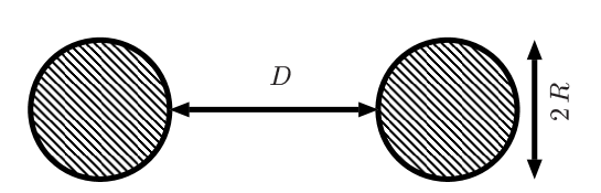
FIG. 1.: The geometry of two equal neighboring spheres.

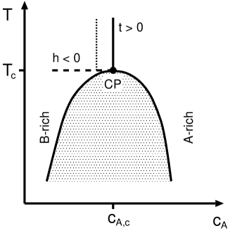
FIG. 2.: Schematic phase diagram of a binary liquid mixture consisting of $A$ and $B$ particles in terms of temperature $T$ and concentration $c_{A}$ of $A$ particles. The shaded area is the two phase region $-$ ending in the critical point $CP$ $-$ which separates the A-rich and the B-rich phase. The relevant thermodynamic variables near the critical point are $t$ and $h$. Three different thermodynamic paths are indicated as considered in the main text.

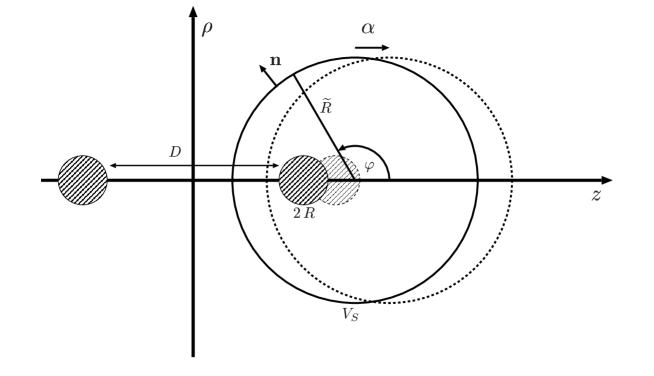
FIG. 4.: Calculating the force via Eq. (39). $\widetilde{R}$ is the radius of a sphere $V_{S}$ that contains one of the spherical particles of diameter $2\,R$. The projection onto the $\rho$-$z$-plane is parametrized with the angle $\varphi$. The interior of $V_{S}$ is shifted by the infinitesimal amount $\alpha$, which is equivalent to an infinitesimal change of the distance $D$ between the two particles.

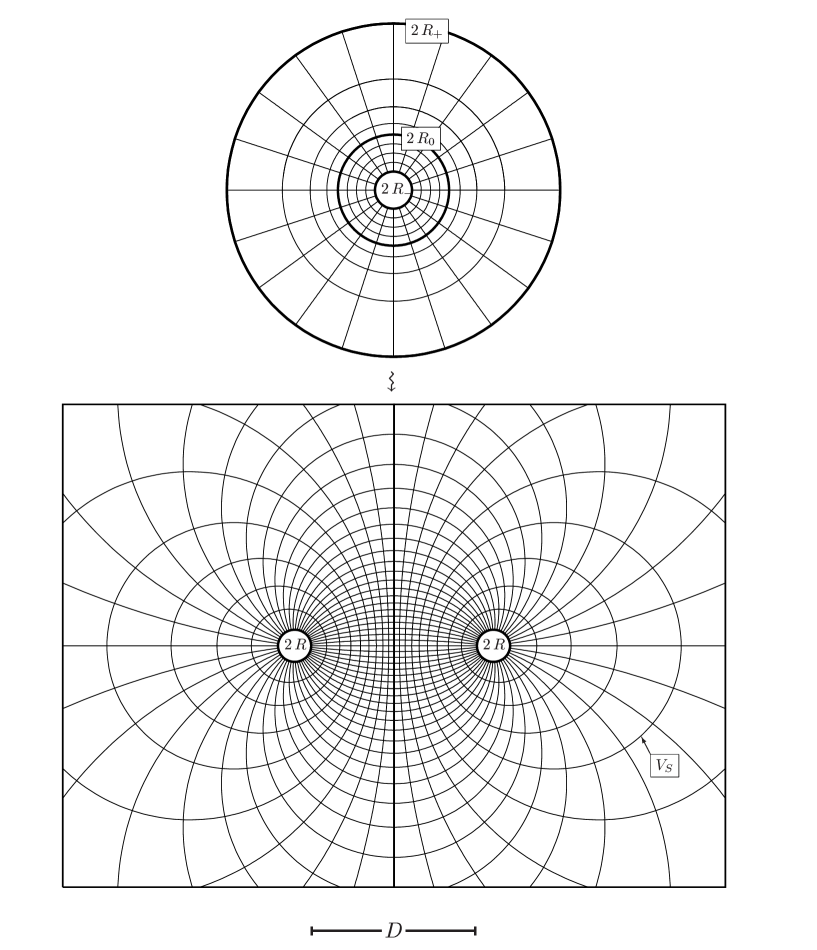
FIG. 3.: The conformal lattice (bottom) for two spheres of diameter $2\,R$ at distance $D$ (see Fig. 1) as obtained from the lattice between concentric spheres of diameter $2\,R_{+}$ and $2\,R_{-}$, respectively. (For the purpose of clear visibility here the two lattices are shown on different scales.) The sphere with diameter $2\,R_{0}=2\,\sqrt{R_{+}\,R_{-}}$ is mapped onto the vertical midplane of the conformal lattice. We note that inside the sphere with diameter $2\,R_{0}$ the spherical lattice lines are chosen equidistant and more dense than outside. $R$ and $D$ are given by Eqs. (17) and (18). $V_{S}$ is introduced in Subsec. III D.

FIG. 5.: Force between two particles as function of temperature $T>T_{c}$ and for $H=0$ relative to the force at criticality. The force is maximal for $\Theta_{+}=\Theta_{\rm max}(\Delta)$ as indicated by the dots.

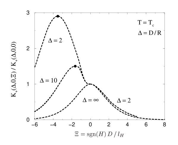
FIG. 6.: Force between two particles as function of the bulk field $H$ at $T=T_{c}$ relative to the force at criticality $(\tau,H)=(0,0)$. The force is maximal for $\Xi=\Xi_{\rm max}(\Delta)$ as indicated by the dots.

FIG. 7.: Maximum force values as function of distance. For small distances the force increases as $\Delta^{-5/2}$ which is scaled out here. Accordingly, the forces are normalized by the value $K_{0}=\lim_{\Delta\to 0}(\Delta^{5/2}K_{+}(\Delta,0,0))$ at the critical point in the limit of vanishing distance. For large distances the forces decay as $\Delta^{-2\,\beta/\nu-1}$, i.e., as $\Delta^{-3}$ within mean-field theory so that $\Delta^{5/2}K_{+}$ decays as $\Delta^{-1/2}$. $\Theta_{+}=D/\xi_{+}$ and $\Xi=\text{sgn}(H)D/l_{H}$.

FIG. 8.: Force between two particles as function of temperature for fixed compositions $c_{A}\neq c_{A,c}$ which implies fixed values of ${m_{b}}^{\ast}=m_{b}\,D^{\beta/\nu}$. Considering the dotted path in Fig. 2, i.e., for $m_{b}=\text{const}$ [for a relation between $m_{b}$ and $M_{b}\sim(c_{A}-c_{A,c})$ see, c.f., Eq. (63)] both thermodynamic variables $\tau$ and $H$ and thus both scaling variables $\Theta_{+}=D/\xi_{+}$ and $\Xi=\text{sgn}(H)D/l_{H}$ are varied simultaneously [see, c.f., Eq. 61]. The Casimir force increases by going further away from the critical composition.

FIG. 9.: Comparison of dispersion forces and Casimir forces at the critical point ($T=T_{c},c_{A}=c_{A,c}$) as function of the distance $D$ in units of the sphere radius $R$. The forces are shown for both a sphere in front of a planar wall (SW) and for two spherical particles (SS). For a detailed discussion see the main text.

FIG. 10.: Normalized scaling function $K_{+}^{||}$ of the force for a film with thickness $L$ at $T_{c}$, i.e., $\Theta_{+}=L/\xi_{+}=0$ as function of the scaling variable $\Xi=\text{sgn}(H)\,L/l_{H}$.

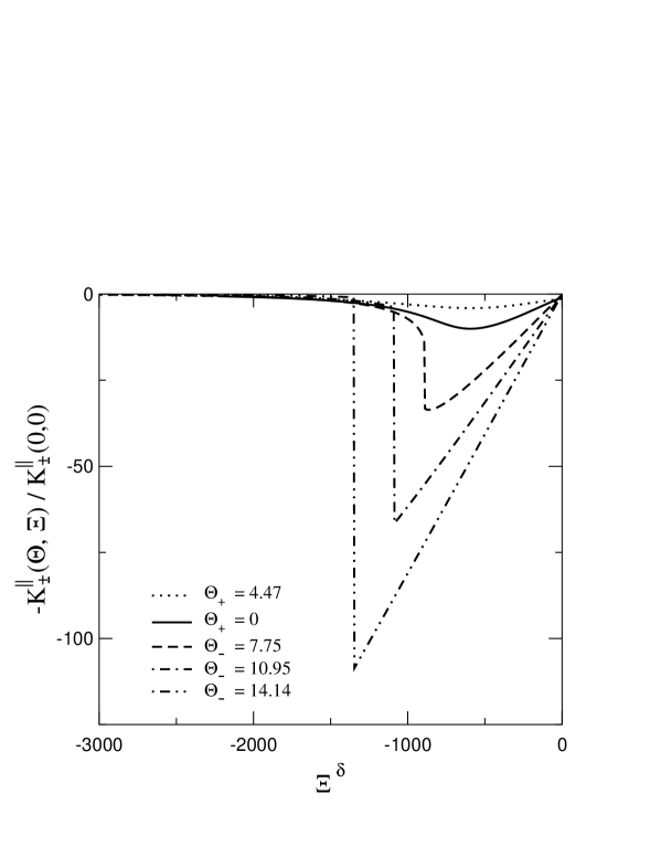
FIG. 11.: Normalized scaling function $K_{\pm}^{||}$ of the force between parallel plates at distance $L$ for different temperatures, i.e., different values of the scaling variable $\Theta_{\pm}=L/\xi_{\pm}$ as function of the bulk field $H$. Note that the scaling variable $\Xi=\text{sgn}(H)\,L/l_{H}$ raised to the power $\delta$, where $\delta=3$ within mean-field theory, is directly proportional to $H$ revealing the almost linear dependence of the force on $H$ over a wide range of values. For details see the main text.

FIG. 12.: Pairs of density profiles coexisting at capillary condensation for various temperatures $T<T_{c}$ relative to the bulk order parameter $m_{b}^{cp}$ at the capillary critical point. The lower curves are stable further away from bulk coexistence whereas for the upper ones capillary condensation has taken place. Above the critical point of capillary condensation (see Fig. 13) the profiles look similar to the upper ones.

FIG. 13.: Phase diagram for capillary condensation as obtained within the present mean field approach. The transition line ends in the capillary critical point ($\Theta_{-}=7.17,\Xi=-9.54$). The straight line ending at ($\Theta_{-}=0,\Xi=0$) is the line of first-order phase transitions in the bulk.

FIG. 14.: The difference $\delta K_{-}^{||}$ between the force values of profiles coexisting at capillary condensation (solid line) and an approximate expression thereof (dashed line). The overall $L$ dependence of the forces ($L^{-4}$) is scaled out in $K_{-}^{||}$, $\delta K_{-}^{||}$, and the approximation.

REFERENCES

- [1] M. E. Fisher and P. G. de Gennes, C. R. Acad. Sc. Paris B 287: 207 (1978).
- [2] This conjecture has been worked out in more detail in P. G. de Gennes, C. R. Acad. Sci. Ser. II 292: 701 (1981).
- [3] D. Beysens and D. Estève, Phys. Rev. Lett. 54: 2123 (1985); for a review see D. Beysens, J.-M. Petit, T. Narayanan, A. Kumar, and M. L. Broide, Ber. Bunsenges. Phys. Chem. 98: 382 (1994).
- [4] P. D. Gallagher, M. L. Kurnaz, and J. V. Maher, Phys. Rev. A 46: 7750 (1992); M. L. Kurnaz and J. V. Maher, Phys. Rev. E 51: 5916 (1995).
- [5] B. M. Law, J.-M. Petit, and D. Beysens, Phys. Rev. E 57: 5782 (1998); J.-M. Petit, B. M. Law, and D. Beysens, J. Colloid Interface Sci. 202: 441 (1998).
- [6] T. Narayanan, A. Kumar, E. S. R. Gopal, D. Beysens, P. Guenoun, and G. Zalczer, Phys. Rev. E 48: 1989 (1993).
- [7] Y. Jayalakshmi and E. W. Kaler, Phys. Rev. Lett. 78: 1379 (1997).
- [8] H. Grüll, D. Woermann, Ber. Bunsenges. Phys. Chem. 101: 814 (1997).
- [9] W. B. Russel, D. A. Saville, and W. R. Schowalter, Colloidal Dispersions (Cambridge University Press, Cambridge, 1989).
- [10] Colloid Physics: Proceedings of the Workshop on Colloid Physics held at the University of Konstanz, Germany, November 30 - December 2, 1995, Physica A 235 (1997).
- [11] F. Schlesener, A. Hanke, R. Klimpel, and S. Dietrich, Phys. Rev. E 63: 041803 (2001).
- [12] C. N. Likos, Phys. Rep. 348: 267 (2001).
- [13] H. Löwen, Phys. Rev. Lett. 74: 1028 (1995); Z. Phys. B 97: 269 (1995).
- [14] T. Bieker and S. Dietrich, Physica A 252: 85 (1998); and references therein.
- [15] C. Bauer, T. Bieker, and S. Dietrich, Phys. Rev. E 62: 5324 (2000).
- [16] U. Brodatzki and K. Mecke, preprint cond-mat/0112009.
- [17] H. B. G. Casimir, Proc. K. Ned. Akad. Wet. 51: 793 (1948).
- [18] S. K. Lamoreaux, Am. J. Phys. 67: 850 (1999).
- [19] G. Bressi, G. Carugno, R. Onofrio, and G. Ruoso, Phys. Rev. Lett. 88: 041804 (2002).
- [20] K. Symanzik, Nucl. Phys. B190: 1 (1981).
- [21] P. Ziherl, R. Podgornik, and S. Žumer, Phys. Rev. Lett. 82: 1189 (1999); A. Borštnik, H. Stark, and S. Žumer, Phys. Rev. E 61: 2831 (2000).
- [22] N. Uchida, Phys. Rev. Lett. 87: 216101 (2001).
- [23] P. Ziherl and I. Muševič, Liq. Cryst. 28: 1057 (2001).
- [24] J. O. Indekeu, M. P. Nightingale, and W. V. Wang, Phys. Rev. B 34: 330 (1986).
- [25] M. Krech and S. Dietrich, Phys. Rev. Lett. 66: 245 (1991); 67: 1055 (1991); Phys. Rev. A 46: 1922 (1992); 46: 1886 (1992); J. Low Temp. Phys. 89: 145 (1992).
- [26] M. Krech, The Casimir Effect in Critical Systems (World Scientific, Singapore, 1994); J. Phys.: Condens. Matter 11: R391 (1999).
- [27] M. Krech, Phys. Rev. E 56: 1642 (1997).
- [28] M. Kardar and R. Golestanian, Rev. Mod. Phys. 71: 1233 (1999).
- [29] A. Mukhopadhyay and B. M. Law, Phys. Rev. Lett. 83: 772 (1999).
- [30] R. Garcia and M. H. W. Chan, Phys. Rev. Lett. 83: 1187 (1999); Physica B 280: 55 (2000); J. Low Temp. Phys. 121: 495 (2000); Phys. Rev. Lett. 88: 086101 (2002).
- [31] The same holds for one- or two-component fluids near their liquid-vapor critical points.
- [32] K. Binder, in Phase Transitions and Critical Phenomena, edited by C. Domb and J. L. Lebowitz (Academic, London, 1983), Vol. 8, p. 1.
- [33] H. W. Diehl, in Phase Transitions and Critical Phenomena, edited by C. Domb and J. L. Lebowitz (Academic, London, 1986), Vol. 10, p. 75; H. W. Diehl, Int. J. Mod. Phys. B 11: 3503 (1997).
- [34] A. J. Liu and M. E. Fisher, Phys. Rev. A 40: 7202 (1989).
- [35] J. L. Cardy, Phys. Rev. Lett. 65: 1443 (1990).
- [36] H. W. Diehl and M. Smock, Phys. Rev. B 47: 5841 (1993); 48: 6740 (1993).
- [37] E. Eisenriegler and M. Stapper, Phys. Rev. B 50: 10009 (1994).
- [38] G. Flöter and S. Dietrich, Z. Phys. B 97: 213 (1995).
- [39] For a review see B. M. Law, Prog. Surf. Sci. 66: 159 (2001).
- [40] A. Hanke and S. Dietrich, Phys. Rev. E 59: 5081 (1999).
- [41] A. Hanke, Phys. Rev. Lett 84: 2180 (2000).
- [42] H. W. Diehl and M. Smock, Physica A 281: 268 (2000); Eur. Phys. J. B 21: 567 (2001).
- [43] A. Hanke and M. Kardar, Phys. Rev. Lett. 86: 4596 (2001); preprint cond-mat/0110532.
- [44] T. W. Burkhardt and E. Eisenriegler, Phys. Rev. Lett. 74: 3189 (1995); 78: 2867 (1997).
- [45] R. Netz, Phys. Rev. Lett. 76: 3646 (1996).
- [46] A. Hanke, F. Schlesener, E. Eisenriegler, and S. Dietrich, Phys. Rev. Lett. 81: 1885, (1998).
- [47] T. W. Burkhardt and E. Eisenriegler, J. Phys. A 18: L83 (1985).
- [48] S. Gnutzmann and U. Ritschel, Z. Phys. B 96: 391 (1995).
- [49] E. Eisenriegler and U. Ritschel, Phys. Rev. B 51: 13717 (1995).
- [50] M. E. Fisher, Rev. Mod. Phys. 46: 597 (1974); 70: 653 (1998).
- [51] M. E. Fisher and P. J. Upton, Phys. Rev. Lett. 65: 2402 (1990).
- [52] M. E. Fisher and P. J. Upton, Phys. Rev. Lett. 65: 3405 (1990).
- [53] Z. Borjan and P. J. Upton, Phys. Rev. Lett. 81: 4911 (1998).
- [54] Z. Borjan and P. J. Upton, Phys. Rev. E 63: 065102 (2001).
- [55] I. S. Gradshteyn and I. M. Ryzhik, Table of Integrals, Series, and Products (Academic, London, 1965).
- [56] M. E. Fisher and H. Au-Yang, Physica A 110: 255 (1980).
- [57] R. L. Burden and J. D. Faires, Numerical Analysis (PWS, Boston, 1993).
- [58] H. Späth, Eindimensionale Spline-Interpolations-Algorithmen (Oldenbourg, 1990); H. Späth, Zweidimensionale Spline-Interpolations-Algorithmen (Oldenbourg, 1991).
- [59] L. S. Brown, Ann. of Phys. 126: 135 (1980).
- [60] B. V. Derjaguin, Kolloid Z. 69: 155 (1934).
- [61] E. Eisenriegler, A. Hanke, and S. Dietrich, Phys. Rev. E 54: 1134 (1996).
- [62] J. Chen and A. Anandarajah, J. Colloid Interface Sci. 180: 519 (1996).
- [63] B. Widom, J. Chem. Phys. 43: 3898 (1965).
- [64] H. B. Tarko and M. E. Fisher, Phys. Rev. Lett. 31: 926 (1973); Phys. Rev. B 11, 1217 (1975).
- [65] N. B. Wilding and M. Krech, Phys. Rev. E 57: 5795 (1998).
- [66] A. M. Ferrenberg, D. P. Landau, and K. Binder, Phys. Rev. E 58: 3353 (1998).
- [67] A. Drzewińzki, A. Maciołek, and R. Evans, Phys. Rev. Lett. 85: 3079 (2000); A. Maciołek, A. Drzewińzki, and R. Evans, Phys. Rev. E 64: 056137 (2001).
- [68] H. Nakanishi and M. E. Fisher, J. Chem. Phys. 78: 3279 (1983).