Density of States in a Mesoscopic SNS Junction Density of States in a Mesoscopic SNS Junction

P. M. Ostrovsky, M. A. Skvortsov, M. V. Feigel’man Ostrovsky, Skvortsov, Feigel’man

Density of States in a Mesoscopic SNS Junction

Abstract

Semiclassical theory of proximity effect predicts a gap $E_{\rm g}\sim\hbar D/L^{2}$ in the excitation spectrum of a long diffusive superconductor/normalmetal/superconductor (SNS) junction. Mesoscopic fluctuations lead to anomalously localized states in the normal part of the junction. As a result, a nonẓero, yet exponentially small, density of states (DOS) appears at energies below $E_{\rm g}$. In the framework of the supermatrix nonlinear $\sigma$ṃodel these prelocalized states are due to instanton configurations with broken supersymmetry. The exact result for the DOS near the semiclassical threshold is found provided the dimensionless conductance of the normal part $G_{\rm N}$ is large. The case of poorly transparent interfaces between the normal and superconductive regions is also considered. In this limit the total number of the subgap states may be large.

73.21.-b, 74.50.+r, 74.80.Fp

1. Introduction. It has recently been shown within several different although related contexts that the excitation energy spectrum of SuperconductiveNormal (SN) chaotic hybrid structures [1, 2] and superconductors with magnetic impurities [3, 4] does not possess a hard gap as predicted by a number of papers [5, 6, 7, 8] using the semiclassical theory of superconductivity [9, 10, 11]. With mesoscopic fluctuations taken into account, the phenomenon of soft gap appears: the density of states is nonzero at all energies, but it decreases exponentially fast below the semiclassical threshold $E_{\rm g}\sim\hbar/\tau_{c}$, with $\tau_{c}$ being the characteristic dwell time in the N region. In particular, for diffusive systems perfectly connected to a superconductor, $E_{\rm g}$ has the order of the Thouless energy $E_{\rm Th}$ in the N region [5, 6].

The first result in this direction was obtained in Ref. [1], where the subgap DOS in a quantum dot was studied by employing the universality hypothesis and the predictions [12] of the random matrix theory (RMT) [13]. Later on, the tail states in a superconductor with magnetic impurities were analysed in Refs. [3, 4] on the basis of the supersymmetric nonlinear $\sigma$ṃodel method [14] extended to include superconductive paring [15].

Fully microscopic approach to the problem of the subgap states in diffusive NS systems was developed in Ref. [2] in the framework of the supersymmetric $\sigma$ṃodel similar to that employed in Refs. [3, 4]. Physically, the lowḷying excitations in SN structures are due to anomalously localized eigenstates [16] in the N region. From the mathematical side, nonzero DOS at $E<E_{\rm g}$ comes about when nontrivial field configurations -instantons -are taken into account in the $\sigma$ṃodel functional integral. As shown in [2], at $E\approx E_{\rm g}$ there are two different types of instantons, their actions being different by the factor 2. The main contribution to the exponentially small subgap DOS is determined by the Gaussian integral near the leastạction instanton.

For a planar (quasi1̣D) SNS junction with ideally transparent SN interfaces it is given by (provided $G_{\rm N}^{-2/3}\ll\varepsilon\ll 1$)

$$\left<\rho\right>=0.97\delta^{-1}G_{\rm N}^{-1/2}\varepsilon^{-1/4}\exp\left[-1.93G_{\rm N}\varepsilon^{3/2}\right],$$ (1)

where $\varepsilon=(E_{\rm g}-E)/E_{\rm g}$, $G_{\rm N}=4\pi\nu DL_{y}L_{z}/L_{x}\gg 1$ is the dimensionless conductance (in units of $e^{2}/2\pi\hbar$) of the normal part connecting two superconductors, $E_{\rm g}=3.12E_{\rm Th}$, $E_{\rm Th}=D/L_{x}^{2}$ is the Thouless energy, and $\delta=(\nu V)^{-1}$ is the mean level spacing. Here $L_{x}$ is the thickness of the N region, assumed to be larger than the superconductive coherence length. It is also assumed that the lateral dimensions $L_{y},L_{z}$ are not much larger than $L_{x}$ (otherwise, the instanton solution acquires additional dimension(s) and the exponent $3/2$ changes, cf. [2] for details). The corresponding meanf̣ield (MF) expression above the gap reads [6]

$$\left<\rho\right>_{\rm MF}=3.72\delta^{-1}\sqrt{|\varepsilon|}.$$ (2)

Generally, the functional form of Eqs. (1), (2) is retained, whereas the coefficients are geometryḍependent and can be found from the solution of the standard Usadel equation [11] for the specific sample geometry. In any case, the total number of states with energies below $E_{\rm g}$ is of the order of one.

In the present Letter we extend our previous results [2] in two different directions. Firstly, we derive exact expression for the DOS in the energy region $|\varepsilon|\ll 1$, without using anymore the inequality $\varepsilon\gg G_{\rm N}^{-2/3}$. The obtained result interpolates smoothly between the semiclassical squareṛoot edge (2) and exponential tail (1). Secondly, we consider the same SNS system allowing for nonịdeal transparencies at the SN interfaces. The result depends upon the relation between dimensionless interface conductance $G_{\rm T}$ and normal conductance $G_{\rm N}$. As long as $G_{\rm T}\geq G_{\rm N}^{1/4}$, all qualitative features of the previous solution are retained, but the value of the semiclassical threshold $E_{\rm g}$ and numerical coefficients in the expression like (1) become dependent upon the value of $t\equiv G_{\rm T}/G_{\rm N}$. However, at further decrease of interface transparency, $G_{\rm T}\ll G_{\rm N}^{1/4}$, the DOS behaviour changes dramatically: in the semiclassical region $E>E_{\rm g}$ it acquires the inverseṣquareṛoot singularity, $\left<\rho\right>_{\rm MF}\sim(-\varepsilon)^{-1/2}$. At smallest $|\varepsilon|$ this singularity smoothens out and crosses over to an exponentially decaying tail of lowẹnergy states. Distinctive feature of this tail, as opposed to the situations discussed previously, is that the total number of subgap states becomes large and grows as $G_{\rm T}^{-1/2}G_{\rm N}^{1/8}\gg 1$. We coined this situation as “strong tail”, and find exponential asymptotics of the DOS in the strong tail region.

2. Outline of the method. We treat the problem within the supersymmetric formalism. The derivation of the $\sigma$ṃodel functionalịntegral representation can be found in Refs. [14, 15, 17]. The DOS is given by the integral over the supermatrix $Q$:

$$\left<\rho(E,{\bf r})\right>=\frac{\nu}{4}\Real\int\operatorname{str}(k\Lambda Q({\bf r}))e^{-{\cal S}[Q]}{\cal D}Q,$$ (3)

$${\cal S}[Q]=\frac{\pi\nu}{8}\int d{\bf r}\;\operatorname{str}\left[D(\nabla Q)^{2}+4iQ(\Lambda E+i\tau_{x}\Delta)\right].$$ (4)

$Q$ is an $8\times 8$ matrix operating in Nambu, timeṛeversal and BoseFermi (supersymmetry) spaces. Pauli matrices operating in Nambu and TR spaces are denoted $\tau_{i}$ and $\sigma_{i}$. The matrix $k$ is the third Pauli matrix in FB space. $\Lambda=\tau_{z}\sigma_{z}$. Integration in (3) runs over the manifold $Q^{2}=1$ with the additional constraint

$$Q=CQ^{T}C^{T},\qquad C=-\tau_{x}\begin{pmatrix}i\sigma_{y}&0\\ 0&\sigma_{x}\end{pmatrix}_{\rm FB}.$$ (5)

This manifold is parameterized by 8 commuting and 8 anticommuting variables. It turns out however that only 4 commuting and 4 anticommuting modes are relevant in the vicinity of the quasiclassical gap while contributions from all other modes to the DOS cancel. The detailed discussion of this fact will be published elsewhere [17]. The reduced parameterization for the commuting part of $Q$ in terms of the 4 variables reads [2]:

$$Q_{c}^{\rm BB} =[\sigma_{z}\cos k_{\rm B}+\tau_{z}\sin k_{\rm B}(\sigma_{x}\cos\chi_{\rm B}+\sigma_{y}\sin\chi_{\rm B})]$$

$$\times[\tau_{z}\cos\theta_{\rm B}+\sigma_{z}\tau_{x}\sin\theta_{\rm B}],$$ (6)

$$Q_{c}^{\rm FF} =\tau_{z}\sigma_{z}\cos\theta_{\rm F}+\tau_{x}\sin\theta_{\rm F}.$$

The commuting part of the action (with all Grassmann variables being zero) is simplified by introducing new variables $\alpha=(\theta_{\rm B}+k_{\rm B})/2$, $\beta=(\theta_{\rm B}-k_{\rm B})/2$. Then the action (4) for the normal part ($\Delta=0$) takes the form

$$S[\theta_{\rm F},\alpha,\beta]=2S_{0}[\theta_{\rm F}]-S_{0}[\alpha]-S_{0}[\beta],$$ (7)

$$S_{0}[\theta]=\frac{\pi\nu}{4}\int d{\bf r}\;\left[D(\nabla\theta)^{2}+4iE\cos\theta\right].$$ (8)

Variation of this action yields the identical Usadel equations for $\theta_{\rm F}$, $\alpha$, and $\beta$:

$$D\nabla^{2}\theta+2iE\sin\theta=0,$$ (9)

with the boundary conditions $\theta(\pm L_{x}/2)=\pi/2$. Eq. (9) generally possesses two different solutions $\theta_{1,2}=\pi/2+i\psi_{1,2}$ which coincide ($\psi_{1,2}({\bf r})=\psi_{0}({\bf r})$) just at the threshold energy $E_{\rm g}$, and are close to each other in the range $|\varepsilon|\ll 1$ we are interested in. Thus there are 8 possible saddle points for the action (7) corresponding to two solutions of the Usadel equation for each variable $\theta_{\rm F},\alpha,\beta$. Rotation over the angle $\chi_{\rm B}\in[0,2\pi)$ connects some of them and produces the whole degenerate family of saddle points (see Refs. [2, 17] for details). In the following, we will need the function $f_{0}({\bf r})$ which is the normalized difference $\psi_{2}({\bf r})-\psi_{1}({\bf r})$ at $E\to E_{\rm g}$; it obeys the linear equation

$$D\nabla^{2}f_{0}+2E_{\rm g}\sinh\psi_{0}\,f_{0}=0.$$ (10)

3. Exact result for the transparent interface. For energies close to $E_{\rm g}$ we substitute $\theta=\pi/2+i\psi_{0}+igf_{0}$ into (8), expand it in powers of $g$ and $\varepsilon$ and integrate over space using (10):

$$S_{0}[\theta]=S_{0}[\pi/2+i\psi_{0}]+\tilde{G}\left[-\tilde{\varepsilon}g+\frac{g^{3}}{3}\right],$$ (11)

$$\tilde{G}=\frac{\pi c_{2}E_{\rm g}}{2\delta},\quad\tilde{\varepsilon}=\frac{2c_{1}}{c_{2}}\varepsilon,$$

where we have introduced the constants $c_{n}=\int(d{\bf r}/V)f_{0}^{2n-1}\cosh\psi_{0}$. For the quasi1̣D geometry, $c_{1}=1.15$ and $c_{2}=0.88$. To describe deviation of the angles $\alpha$, $\beta$, $\theta_{\rm F}$ from $\pi/2+i\psi_{0}$ we introduce, analogously to $g$, three parameters $u$, $v$, $w$, respectively. Grassmann variables are introduced as $Q=e^{-iW_{c}/2}e^{-iW_{a}/2}\Lambda e^{iW_{a}/2}e^{iW_{c}/2}$ where $Q_{c}=e^{-iW_{c}/2}\Lambda e^{iW_{c}/2}$ is specified in Eqs. (6) and

$$W_{a}=\begin{pmatrix}0&W_{a}^{\rm FB}\\ i\tau_{x}\sigma_{x}(W_{a}^{\rm FB})^{T}\sigma_{y}\tau_{x}&0\\ \end{pmatrix},$$

as it must satisfy the antiselfconjugate condition $W_{a}+CW_{a}^{T}C^{T}=0$. Finally,

$$W_{a}^{\rm FB}=\frac{f_{0}}{4}\begin{pmatrix}0&\zeta-\lambda&\zeta+\lambda&0\\ -\zeta+\lambda&0&0&-\zeta-\lambda\\ \xi+\eta&0&0&\xi-\eta\\ 0&-\xi-\eta&-\xi+\eta&0\\ \end{pmatrix}.$$

Expanding the action in $u$, $v$, $w$ and Grassmann variables leads to

$${\cal S}=\tilde{G}\biggl{[}\tilde{\varepsilon}(u+v-2w)-\frac{u^{3}+v^{3}-2w^{3}}{3}\\ -\zeta\xi\frac{u+w}{4}-\lambda\eta\frac{v+w}{4}\biggr{]}.$$ (12)

For calculating the DOS we also need an expansion of the preẹxponential factor in (3) as well as the Jacobian $J$ for the parameterization of the $Q$ṃatrix:

$$\frac{\nu}{4}\int d{\bf r}\;\operatorname{str}(k\Lambda Q)=-\frac{ic_{1}}{2\delta}(u+v+2w),$$

$$J=\frac{8i\tilde{G}^{2}}{\pi}|u-v|.$$

Integrating over Grassmann variables and the cyclic angle $\chi_{\rm B}$, performing a rescaling $(u,v,w)\to(2\tilde{G})^{-1/3}(u,v,w)$ which excludes $\tilde{G}$ from the integrand, and changing the variables to $l=(u+v)/2$, $m=(u-v)^{2}/2$, we arrive at the following expression for the integral DOS:

$$\left<\rho\right>=\frac{c_{1}(2\tilde{G})^{-1/3}}{4\pi\delta}\Real\int\limits_{0}^{\infty}dm\int dl\,dw\;(w+l)\\ \times(w^{2}+2lw+l^{2}-m)\exp\left[-\frac{w^{3}}{3}+\epsilon w+\frac{l^{3}}{3}+ml-\epsilon l\right]\!,$$ (13)

where we introduced the notation $\epsilon=(2\tilde{G})^{2/3}\tilde{\varepsilon}.$

At this stage we have to choose the contours of integration over $w$ and $l$. The usual convergence requirements for the nonexpanded action (7) enforce the contour for $w$ ($l$) go along the imaginary (real) axis at large values of $w$ ($l$). However since the main contribution to the DOS comes from the expression (13) determined by small $w$ and $l$, these contours should be properly deformed to achieve convergence of (13). The integral (13) converges if the contour for $l$ runs to infinity in the dark regions in Fig. 1 and otherwise for $w$. Therefore, we should choose the contour $C_{1}$ for $w$ (see Fig. 1), whereas for $l$ there are two possibilities: $C_{2}$ and $C_{3}$. The correct choice is dictated by positivity of the DOS, which imply the contour $C_{3}$ for $l$.

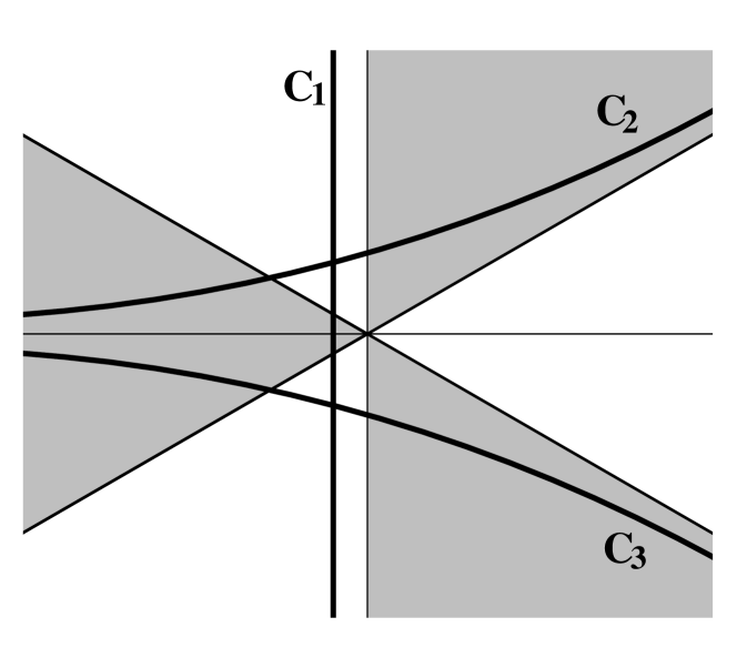
Figure 1: Fig. 1. Possible contours for integration over $w$ and $l$. The proper choice is $C_{1}$ for $w$ and $C_{3}$ for $l$.

Integration in (13) is straightforward although rather cumbersome and leads to the final expression for the DOS:

$$\left<\rho\right>=\frac{2\pi c_{1}}{(2\tilde{G})^{1/3}\delta}\biggl{[}-\epsilon\operatorname{Ai}^{2}(\epsilon)+[\operatorname{Ai}^{\prime}(\epsilon)]^{2}\\ +\frac{\operatorname{Ai}(\epsilon)}{2}\int_{-\infty}^{\epsilon}dy\;\operatorname{Ai}(y)\biggr{]},$$ (14)

where $\operatorname{Ai}(\epsilon)$ is the Airy function. Asymptotic behaviour of the calculated DOS at $\epsilon\gg 1$ coincides with the result (1) of the singleịnstanton approximation [2], see Fig. 2.

Figure 2: Fig. 2. Exact dependence (14) of the DOS on the dimensionless energy $\epsilon$ (solid line). Singleịnstanton approximation (1) (dotted line). Semiclassical result (2) for the DOS (dashed line).

The functional dependence (14) coincides with the RMT prediction for the spectrum edge in the orthogonal ensemble [12]. It is not surprising because the random matrix theory is known to be equivalent to the 0D $\sigma$ṃodel [14]. In our case the problem became effectively 0D when we fixed the coordinate dependence $f_{0}({\bf r})$ for the parameters of $Q$ near $E_{\rm g}$.

Breaking the timeṛeversal symmetry drives the system to the unitary universality class. The corresponding RMT result [12] can be obtained from Eq. (14) by dropping the last integral term. This result can be easily derived by the $\sigma$ṃodel analysis in the following way. Strong magnetic field imposes an additional constraint on the $Q$ṃatrix. As a result the mode associated with the variable $m$ acquires a mass, so, instead of integrating over it we set $m=0$. One of the Grassman modes is also frozen out giving the preẹxponent $(w+l)^{2}$ in the integral (13). Finally, the expression for DoS coincides with Eq. (14) but without the last term.

4. Finite transparency of the NS interface. Now we turn to the analysis of the subg̣ap structure of a quasi1̣D SNS contact with finite conductance $G_{\rm T}$ of the NS boundary. The role of the interface is described by the dimensionless parameter $t=G_{\rm T}/G_{\rm N}$. For $t\gg 1$, the interface is transparent and the result (14) apply. In what follows we will consider the case $t\ll 1$. The effect of finite transparency is described by the additional boundary term [14] in the action

$${\cal S}_{\rm boundary}=-\frac{G_{\rm T}}{16}\operatorname{str}\left(Q^{L}Q^{R}\right),$$ (15)

where $Q^{L,R}$ are the $Q$ṃatrices at both sides of the interface. Eq. (15) is the the first term in the expansion of the general boundary action [14, 4, 18] in the small transparency $\Gamma\ll 1$ of conductive channel and leads to the KupriyanovLukichev [19] boundary conditions. In the diffusive regime ($l\ll L_{x}$) at $t\ll 1$, we have $\Gamma\sim tl/L_{x}$ that justifies the use of Eq. (15). The commuting part of the action can still be written in the form (7) with the additional term in $S_{0}$:

$$S_{0}[\theta]=\frac{\pi\nu L_{y}L_{z}}{4}\int\limits_{-L_{x}/2}^{L_{x}/2}dx\;\left[D(\theta^{\prime})^{2}+4iE\cos\theta\right]\\ -\frac{G_{\rm T}}{4}\sin\left[\theta\left(\frac{L_{x}}{2}\right)\right].$$ (16)

In the limit $t\ll 1$, the Usadel equation has almost space homogeneous solutions, which allows to use an expansion $\psi=A+B[1-4(x/L_{x})^{2}]$ for them. Substituting this ansatz into the action (16), and minimizing over $B$ we obtain the action in terms of $P=e^{A}$:

$$S_{0}(P)=\frac{G_{\rm N}}{8}\left[(s-t)P-\frac{2t}{P}+\frac{t^{2}}{24}P^{2}\right],$$ (17)

where $s=E/E_{\rm Th}$. Here we keep only leading terms and substitute all $s$ except the first one by $t$. After variation we find the cubic saddle point equation for $P$:

$$\frac{s}{t}=1-\frac{2}{P^{2}}-\frac{t}{12}P.$$ (18)

The maximum of the RHS achieved at $P_{0}=(48/t)^{1/3}$ determines the position of the meanf̣ield gap: $s_{\rm g}=t+O(t^{5/3})$ and hence $E_{\rm g}=G_{\rm T}\delta/4\pi$. Depending on the deviation from the threshold, $\varepsilon=(E_{\rm g}-E)/E_{\rm g}=(s_{\rm g}-s)/s_{\rm g}$, there are two regimes for Eq. (18).

Weak tail. If $|\varepsilon|\ll t^{2/3}$ the two solutions of (18) are close to each other and can be seek in the form $P=P_{0}+\delta P$. Expanding the action in powers of $\delta P$ we get

$$S_{0}(P)=S_{0}(P_{0})+\frac{G_{\rm T}}{8}\left[-\varepsilon\delta P+\frac{2}{P_{0}^{4}}(\delta P)^{3}\right].$$ (19)

This equation closely resembles its counterpart (11) for the transparent interface. As mentioned in Ref. [4], this form of the expansion of the action over small deviations near the threshold solution inevitably leads to the instanton action scaling as $\varepsilon^{3/2}$. In fact, there is full equivalence [17] between the DOS for the transparent NS interface given by Eq. (14) and the DOS in the limit $|\varepsilon|\ll t^{2/3}\ll 1$. The latter can be obtained from the former by redefinition of the constants $c_{1,2}$. For a 1D planar contact they appear to be $c_{1}=P_{0}/2$, $c_{2}=6/P_{0}$, $E_{\rm g}/E_{\rm Th}=t$.

In particular, above the threshold, at $\varepsilon<0$, one encounters the meanf̣ield squareṛoot singularity

$$\langle\rho\rangle_{\rm MF}=\frac{4}{\delta}\frac{6^{1/6}}{t^{2/3}}\sqrt{|\varepsilon|}.$$ (20)

The instanton action becomes ${\cal S}=S_{0}(P_{1})-S_{0}(P_{2})=(2/3)6^{1/6}G_{\rm N}t^{1/3}\varepsilon^{3/2}$, and the singleịnstanton asymptotics of the DOS tail reads

$$\left<\rho\right>=\frac{1}{\delta}\sqrt{\frac{\pi 6^{1/6}}{2G_{\rm N}t^{5/3}\sqrt{\varepsilon}}}\exp\left(-\frac{2}{3}6^{1/6}G_{\rm N}t^{1/3}\varepsilon^{3/2}\right).$$ (21)

Strong tail. In the opposite limit, $t^{2/3}\ll|\varepsilon|\ll 1$, the difference between the two solutions for Eq. (18) is large but expansion (17) is still valid (gradients of $\psi_{1,2}$ are small provided $\varepsilon\ll 1$). The roots $P_{1,2}$ can be found neglecting either the second or the third term in Eq. (18): $P_{1}=\sqrt{2/\varepsilon}$, $P_{2}=12\varepsilon/t$, with $P_{2}\gg P_{1}$. Above the threshold that gives the inverseṣquareṛoot singularity in the semiclassical DOS:

$$\left<\rho\right>_{\rm MF}=\frac{2}{\nu}\Real\int d{\bf r}\,\cos\theta=\frac{1}{\delta}\Imag(P-P^{-1})=\frac{1}{\delta}\sqrt{\frac{2}{|\varepsilon|}}.$$ (22)

Below $E_{\rm g}$ one obtains for the instanton action ${\cal S}=-S_{0}(P_{2})=(3/4)G_{\rm N}\varepsilon^{2}$ which determines the oneịnstanton asymptotics of the subgap DOS. The preẹxponent can be calculated by generalizing the method of Ref. [2]. Introducing the deviation parameter $q$ according to $\alpha=\pi/2+i\log P_{2}+iq/\sqrt{2}$ and expanding the action in powers of $q$ and the corresponding Grassmann pair $\zeta\xi$ we obtain for the action and the preẹxponential factor in Eq. (3):

$${\cal S}=\frac{3}{8}G_{\rm N}\varepsilon^{2}\left[2-q^{2}+\frac{q\zeta\xi}{2\sqrt{2}}\right],$$

$$\frac{\nu}{4}\int d{\bf r}\;\operatorname{str}(k\Lambda Q)=-\frac{3i\varepsilon}{t\delta}\left[1-\frac{q}{\sqrt{2}}\right].$$

The measure of integration is ${\cal D}Q=2\sqrt{3/t}(2\varepsilon)^{3/4}dq\,d\zeta\,d\xi$. Inserting these into Eq. (3) we finally obtain

$$\left<\rho\right>=\frac{3}{\delta}\sqrt{\frac{\pi}{G_{\rm N}t^{3}}\sqrt{\frac{\varepsilon^{3}}{2}}}\exp\left(-\frac{3}{4}G_{\rm N}\varepsilon^{2}\right).$$ (23)

5. Discussion. We have considered the integral density of states in a coherent diffusive SNS junction with arbitrary transparency of the SN interface. For the ideal interface ($G_{\rm T}\gg G_{\rm N}$) we managed to go beyond the single-instanton analysis [2] and derived the exact result (14) valid as long as $|E-E_{\rm g}|\ll E_{\rm g}$. This expression uniquely describes the semiclassical square-root DOS (2) above the Thouless gap $E_{\rm g}$, the far subgap tail (1), and the crossover region $\varepsilon\sim G_{\rm N}^{-2/3}$ between the two asymptotics. The functional form of this result coincides with the prediction of the RMT.

As the SN interface become less transparent, $G_{\rm T}\ll G_{\rm N}$, the situation changes. At $G_{\rm T}\gg G_{\rm N}^{1/4}$ these changes are only quantitative: the position of the quasiclassical gap is shifted to $E_{\rm g}=(G_{\rm T}/G_{\rm N})E_{\rm Th}$, but the DOS both above [Eq. (20)] and below [Eq. (21)] the gap has the same dependence on the deviation $\varepsilon$ from $E_{\rm g}$, with the coefficients becoming dependent on $G_{\rm T}$. In this limit, the very far part of the tail [at $\varepsilon\gg(G_{\rm T}/G_{\rm N})^{2/3}$] exhibits another $\varepsilon$-dependence (23), but the corresponding DOS is exponentially small. Therefore, in the limit $G_{\rm T}\gg G_{\rm N}^{1/4}$ the total number of the subgap states is of the order of 1 and is independent on $G_{\rm T}$. We refer to this case as weak tail.

As the interface becomes less transparent, the region of applicability of the weak tail shrinks and finally disappears at $G_{\rm T}\sim G_{\rm N}^{1/4}$. For even lower $G_{\rm T}\ll G_{\rm N}^{1/4}$, the difference between the case of the transparent interface becomes qualitative: the DOS above $E_{\rm g}$ acquires an inverse square-root dependence (22), while the subgap DOS follows (23). In this regime the total number of the subgap states is proportional to $G_{\rm T}^{-1/2}G_{\rm N}^{1/8}\gg 1$ and grows with decreasing $G_{\rm T}$ in contrast to all previous cases when this number is of the order of 1. This indicates that at $G_{\rm T}\sim G_{\rm N}^{1/4}$ the universality class of the problem is changed. At $G_{\rm T}\ll G_{\rm N}^{1/4}$ it is no longer equivalent to the spectral edge of the Wigner-Dyson random matrix ensembles.

The asymptotic results for the DOS above and below the gap, as well as the width of the fluctuation region near $E_{\rm g}$ are summarized in Table I for the three regions considered.

	$\varepsilon<0$	$\varepsilon>0$	$|\varepsilon|_{\rm fluct}$
$t\gg 1$	(2)	(1)	$G_{\rm N}^{-2/3}$
$|\varepsilon|\ll t^{2/3}\ll 1$	(20)	(21)	$G_{\rm N}^{-2/3}t^{-2/9}$
$t^{2/3}\ll|\varepsilon|\ll 1$	(22)	(23)	$G_{\rm N}^{-1/2}$

Table 1: Table I. References to the asymptotic formulas for the DOS above ($\varepsilon<0$) and below ($\varepsilon>0$) the gap, and the width $|\varepsilon|_{\rm fluct}$ of the fluctuation region for the regimes of the transparent interface ($t\gg 1$), weak ($|\varepsilon|\ll t^{2/3}\ll 1$) and strong ($t^{2/3}\ll|\varepsilon|\ll 1$) tails.

Acknowledgements. This research was supported by the SCOPES programme of Switzerland, Dutch Organization for Fundamental Research (NWO), Russian Foundation for Basic Research under grant 01-02-17759, the programme “Quantum Macrophysics” of the Russian Academy of Sciences, and the Russian Ministry of Science.

References

- [1] M. G. Vavilov, P. W. Brower, V. Ambegaokar, and C. W. J. Beenakker, Phys. Rev. Lett. 86, 874 (2001).
- [2] P. M. Ostrovsky, M. A. Skvortsov, and M. V. Feigel’man, Phys. Rev. Lett. 87, 027002 (2001).
- [3] A. Lamacraft and B. D. Simons, Phys. Rev. Lett. 85, 4783 (2000).
- [4] A. Lamacraft and B. D. Simons, Phys. Rev. B64, 014514 (2001).
- [5] A. A. Golubov and M. Yu. Kupriyanov, Zh. Eksp. Teor. Fiz. 96, 1420 (1989) [Sov. Phys. JETP 69, 805 (1989)].
- [6] F. Zhou, P. Charlat, B. Spivak, and B. Pannetier, J. Low Temp. Phys. 110, 841 (1998).
- [7] J. A. Melsen, P. W. Brower, K. M. Frahm, and C. W. J. Beenakker, Europhys. Lett. 35, 7 (1996); Physica Scripta 69, 223 (1997).
- [8] S. Pilgram, W. Belzig, and C. Bruder, Phys. Rev. B62, 12462 (2000).
- [9] G. Eilenberger, Z. Phys. 214, 195 (1968).
- [10] A. I. Larkin and Yu. N. Ovchinnikov, Zh. Eksp. Teor. Fiz. 55, 2262 (1968) [Sov. Phys. JETP 28, 1200 (1969)].
- [11] K. Usadel, Phys. Rev. Lett. 25, 507 (1970).
- [12] C. A. Tracy and H. Widom, Comm. Math. Phys. 159, 151 (1994); 177, 727 (1996).
- [13] M. L. Mehta, Random matrices, Academic, New York, 1991.
- [14] K. B. Efetov, Supersymmetry in Disorder and Chaos, Cambridge University Press, New York, 1997.
- [15] A. Altland, B. D. Simons, and D. TarasṢemchuk, Pis’ma Zh. Eksp. Teor. Fiz. 67, 21 (1997) [JETP Lett. 67, 22 (1997)]; Adv. Phys. 49, 321 (2000).
- [16] B. A. Muzykantskii and D. E. Khmelnitskii, Phys. Rev. B51, 5480 (1995).
- [17] P. M. Ostrovsky, M. A. Skvortsov, and M. V. Feigel’man, Zh. Eksp. Teor. Fiz. to be published
- [18] W. Belzig and Yu. V. Nazarov, Phys. Rev. Lett. 87, 067006 (2001).
- [19] M. Yu. Kuprianov and V. F. Lukichev, Zh. Eksp. Teor. Fiz. 94(6), 139 (1988) [Sov. Phys. JETP, 67, 1163 (1988)].