Quantum Nyquist Temperature Fluctuations

Abstract

We consider the temperature fluctuations of a small object. Classical fluctuations of the temperature have been considered for a long time. Using the Nyquist approach, we show that the temperature of an object fluctuates when in a thermal contact with a reservoir. For large temperatures or large specific heat of the object $C_{v}$, we recover standard results of classical thermodynamic fluctuations $\langle\Delta T^{2}\rangle=\frac{k_{B}T^{2}}{C_{v}}$. Upon decreasing the size of the object, we argue, one necessarily reaches the quantum regime that we call quantum temperature fluctuations. At temperatures below $T^{*}\sim\hbar/k_{B}\tau$, where $\tau$ is the thermal relaxation time of the system, the fluctuations change the character and become quantum. For a nano-scale metallic particle in a good thermal contact with a reservoir, $T^{*}$ can be on a scale of a few Kelvin.

Classical thermodynamic fluctuations have been studied for more than two centuries. The Gibbs canonical distribution function, $P(\alpha)d\alpha\propto\exp[-E(\alpha)/k_{B}T]d\alpha$, is one of the most fundamental concept in statistical physics. All thermodynamic variables can be obtained from this distribution function. According to the initial assertion of Gibbs, the temperature of a canonical ensemble is constant and thus does not fluctuate. Therefore, the temperature fluctuation cannot be generically represented by the above distribution function. Instead it is derived from energy fluctuations ($\delta E$). Alternatively, the von Laue approach LL80 to fluctuating system thermodynamics via the minimal work can also lead to the temperature fluctuation ($\delta T$). In recent years, there has been increasing interest in the nano-scale problems such as the glass transition KTW89 , nucleation Ring2001 , and protein folding Matt00 . Of device importance, the mechanical resonators are being pushed to the nanometer scale CR98 ; CR01 . For these nano-scale systems, the temperature fluctuation can be large. Recently, it has been shown DHS00 that the von Laue approach gives much more reasonable results for the temperature fluctuation in a confined geometry than the treatment with the Gibbs distribution function. To the best of our knowledge, the existing study has been limited to the classical regime. We know that any classical variable, say coordinate, force, etc., has its corresponding standard quantum limit where quantum fluctuations dominate. Similarly, we expect temperature $T$ will have its quantum limit. Here we argue that when the temperature is below $T^{*}\sim\hbar/\tau$, where $\tau$ is the thermal relaxation time of the nano-scale particle, a quantum temperature fluctuation regime emerges.

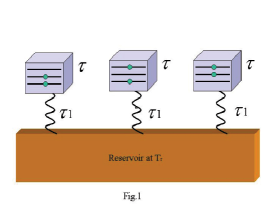
Figure 1: The ensemble of the quantum dots. The thermal relaxation time within each dot is $\tau_{1}$. Each dot is thermally coupled to the reservoir with temperature $T$. Note that each dot contains large enough number of particles that the thermodynamics consideration is still applicable. In particular the notion of a quasi-equilibrium distribution is applicable to each dot. Consider a thermal fluctuation that produces the temperature fluctuation in the $i$th dot, $T+\delta T_{i}$. After the equilibration time $\tau_{1}$, the dot relaxes to the quasi-equilibrium state with temperature $T$. Repeating this measurement on a set of dots, we find the distribution of temperature in an ensemble of dots. The width of this distribution of $T$ will determine the fluctuation of temperature $\delta T$.

Consider an experiment in which we are going to measure the temperature fluctuation of an ensemble of increasingly small objects. Without loss of generality consider a set of quantum dots, as shown in Fig. 1. Assume these dots to be similar in the number of contained particles, size, etc. In addition, each dot has discrete levels, which are filled by a sufficient number ($N\gg 1$) fermions (e.g., electrons) or bosons (e.g., ⁴He atoms). All these dots are in contact with a substrate (large plate) which plays the role of a thermal reservoir. The reservoir is kept at a certain temperature $T$. The thermal contact between the dots and the reservoir will cause the thermal fluctuations in the dots. As a result, the heat flows to/from the reservoir. The relaxation time for the thermal process between the dots and the reservoir is $\tau$.

Let us first briefly recall the derivation of the temperature fluctuation from the von Laue approach LL80 . The propability $w$ for a fluctuation is proportional to $\exp(-R_{min}/k_{B}T)$, where $R_{min}$ is the minimum work needed to fulfill reversibly the given change in the thermodynamic quantities in the quantum dot and $k_{B}$ is Boltzmann’s constant. For simplicity, we assume the volume of each dot be fixed so that $R_{min}=\Delta E-T\Delta S$, where $\Delta E$ and $\Delta S$ are respectively the changes in the energy and entropy. Therefore we have:

$$w=\mathcal{N}_{0}\exp[-\frac{\Delta E-T\Delta S}{k_{B}T}]\;,$$ (1)

where $\mathcal{N}_{0}$ is the normalization constant. For small fluctuations, by expanding $\Delta E$ to the second order in $\Delta S$, and noticing that $\Delta S=(C_{v}/T)\Delta T$ with $C_{v}$ the specific heat, it is found:

$$w=\mathcal{N}_{1}\exp[-\frac{C_{v}\Delta T^{2}}{2k_{B}T}]\;,$$ (2)

where $\mathcal{N}_{1}$ is a new renormalization constant. It follows immediately that the average square fluctuation of temperature at a constant volume is:

$$\langle\Delta T^{2}\rangle=T^{2}/C_{v}\;.$$ (3)

This is the result from the standard classical theory of thermodynamic fluctuations. However, it has to be kept in mind that for the starting equation (1) to be valid, the temperature has to be much bigger than the thermal relaxation rate, i.e.:

$$k_{B}T\gg\hbar/\tau\;,$$ (4)

which also means when the temperature is too low or $\tau$ is too small, the fluctuations can no longer be treated classically.

Here we propose the use of the Nyquist approach Nyquist28 to treat the temperature fluctuation. First consider a generalized coordinate $x$ and its relaxation $\frac{dx}{dt}=-\lambda(x-x_{0})$, where $x_{0}$ is its equilibrium value. The external force $F$, conjugated to the coordinate $x$, determines the equilibrium $x_{0}$. Now, in case there are fluctuations in the external force $F$, equilibrium value $x_{0}={\bar{x}}_{0}+\Delta x_{0}$ fluctuates around its steady state position ${\bar{x}}_{0}$ by $\Delta x_{0}=\frac{\partial x}{\partial F}|_{{\bar{x}}_{0}}\Delta F$. For the equation of motion we get

$$\frac{dx}{dt}=-\lambda(x-{\bar{x}}_{0}-\frac{\partial x}{\partial F}|_{{\bar{x}}_{0}}\Delta F)$$ (5)

Assume now temperature $T=x$ to play the role of a generalized coordinate and the entropy $S=F$ the role of the generalized fluctuating force. The relaxation process of the temperature can be described by a linearized macroscopic “equation of motion”:

$$\frac{d\Delta T}{dt}=-\lambda(\Delta T-\frac{\partial T}{\partial S}|_{{\bar{T}}_{0}}\Delta S)\;,$$ (6)

where $\lambda=1/\tau$, and $\Delta T=T-\bar{T}_{0}$, and is the deviation of the equilibrium temperature $T$ as a result of the fluctuating force $\Delta S$. Equation (6) is valid for the positive time and can be extended to the negative time by changing sign of the derivative. Performing the Fourier transform for $\Delta T$

$$\Delta T(t)=\frac{1}{2\pi}\int d\omega\Delta T_{\omega}e^{-i\omega t}\;,$$ (7)

and similarly for $\Delta S$, we can arrive at

$$\Delta T_{\omega}=\alpha(\omega)\Delta S_{\omega}\;,$$ (8)

where the response function or generalized susceptibility reads:

$$\alpha(\omega)=\frac{\lambda T}{C_{v}(-i\omega+\lambda)}\;,$$ (9)

where we have used $\frac{\partial T}{\partial S}|_{{\bar{T}}_{0}}=\frac{T}{C_{v}}$. Using the fluctuation-dissipation theorem as developed by Callen and Welton, which relates the fluctuation of a thermodynamic quantity to the imaginary part of the susceptibility $\alpha(\omega)$ LL80 ; Callen51 ; GP87 , it immediately follows:

$$\langle\Delta T^{2}\rangle_{\omega}=\hbar\coth(\hbar\omega/2k_{B}T)\alpha^{\prime\prime}(\omega)\;,$$ (10)

where the imaginary part of $\alpha(\omega)$:

$$\alpha^{\prime\prime}(\omega)=\frac{\lambda T}{C_{v}}\frac{\omega}{\omega^{2}+\lambda^{2}}\;.$$ (11)

For the average quadratic fluctuation of $T$, it can be found:

$$\langle\Delta T^{2}\rangle=\frac{\hbar\lambda T}{2\pi C_{v}}\int_{-\infty}^{\infty}d\omega\frac{\omega}{\omega^{2}+\lambda^{2}}\coth(\hbar\omega/2k_{B}T)\;.$$ (12)

The integral on the right side of Eq. (12) depends on the ratio of $k_{B}T/\hbar\lambda$. When $k_{B}T/\hbar\lambda\gg 1$, by expanding $\coth(\hbar\omega/2k_{B}T)=2k_{B}T/\hbar\omega+\hbar\omega/6k_{B}T$ for $\hbar\omega/2k_{B}T\ll 1$, we have

$$\langle\Delta T^{2}\rangle=\frac{k_{B}T^{2}}{C_{v}}\left[1+\frac{\hbar\lambda}{\pi k_{B}T}\ln\frac{\hbar\omega_{c}}{k_{B}T}\right]\;,$$ (13)

where we have introduced an upper band cutoff $\omega_{c}\sim 1/\tau_{1}$ on the order of the relevant bandwidth since at the high frequency the integral $\int_{0}^{\omega_{c}}d\omega\frac{\omega}{\omega^{2}+\eta^{2}}=\ln(\omega_{c}/\eta)$ is logarithmically divergent as $\omega_{c}\rightarrow\infty$. One can recognize immediately that Eq. (13) is the classical limit of the temperature fluctuations as derived above from the von Laue approach. In the opposite limit of low temperatures, $\hbar\lambda\gg k_{B}T$, one finds:

$$\langle\Delta T^{2}\rangle=\frac{\hbar\lambda T}{\pi C_{v}}\ln\frac{\omega_{c}}{\lambda}\;.$$ (14)

Therefore, we find that at low temperatures the temperature fluctuations would acquire a distinctly quantum character with $\hbar/\tau$ entering into the magnitude of $\langle\Delta T^{2}\rangle$. From ergodicity assumption, it follows that the time averaged temperature of each particular dot is equal to the average value of $T$. Any fluctuation, described by Eq.(14), happen on a characteristic time scale $\tau$.

The high temperature expansion in Eq. (13) has already indicated the crossover temperature

$$T^{*}=\frac{\hbar\lambda}{k_{B}\pi}\ln\frac{\omega_{c}}{\lambda}\;,$$ (15)

at which there is a change of the regime from the classical to quantum fluctuations. Physically, $T^{*}\approx\hbar/k_{B}\tau$ corresponds to the uncertainty in energy associated with the relaxation process in the subsystem. The reservoir is attached to a subsystem via a thermal contact that has its own bandwidth $\hbar/\tau$ and any temperature fluctuation will relax on the scale of $\tau$. Once $T\ll T^{*}$, the intrinsic bandwidth of the contact rather than the temperature will dominate the Gaussian fluctuations. As stressed in Ref. LL80 , fluctuations cannot be treated classically if a fluctuating quantity is changing too rapidly or if the subsystems are too small.

Our derivation, which is essentially identical to the classical to quantum Nyquist crossover in the standard Nyquist theory, provides the description of a quantum regime of the temperature fluctuations. There are few possible limitations of this description. One is that our approach in not applicable to the systems outside of thermal equilibrium, say hot electrons and cold phonon bath, as sometimes is the case. Another restriction is that the typical energy level spacing $\delta\sim 1/L^{d}$, $d$ is the dimensionality of the dots, should be small compared to $T$. If the temperature is much smaller than the level spacing, there will be no thermally excited states and the notion of the thermodynamic equilibrium is not applicable to this system. We should also point out that for small particles there are mesoscopic corrections to the total energy of particle, that can be related to the temperature fluctuations. These mesoscopic fluctuations have a typical temperature scale given by Thouless energy $k_{B}T_{Th}=D/L^{2}$, $L$ - is the typical size of the particle, $D$- is diffusion coefficient, and occur in addition to the fluctuations we consider here. We assume here that $T^{*}>T_{Th}$.

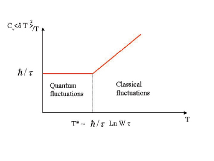
Figure 2: Temperature dependence of the fluctuations $\delta T$. As $T\gg T^{*}$, the classical regime is recovered. As the temperature gets smaller or the subsystem is getting smaller, a quantum fluctuation regime comes into play. Note that the specific heat $C_{v}$ ($\sim T$ for fermions and $\sim T^{3}$ for phonons at low temperature) is temperature dependent.

Experiments on the temperature-dependent fluctuations of magnetization of small paramagnet were performed by Chui et al. Chui92 . Experimentally observed spectral density $\langle\Delta T^{2}\rangle_{\omega}$ was shown to be of the form given by the high temperature expansion of Eq. (10). The thermal relaxation time was $\tau\sim 1$ second for the considered size of the paramagnet (about 1 cm³). The total temperature fluctuation $\langle\Delta T^{2}\rangle=T^{2}/C_{v}$ was also claimed as a result of the integration over Eq. (10). Therefore we can regard this result as an experimental evidence for the classical temperature fluctuation in the canonical ensemble according to Eq. (10). The obvious next step is to extend these measurements to the samples of much smaller sizes, down to 1 $\mu$m in its linear size and study the temperature dependence of the fluctuation spectrum at low temperatures.

Now let us estimate the crossover temperature $T^{*}$ for a metallic dot and for a ⁴He droplet. The low temperature limit $T\ll\hbar\lambda/k_{B}$ implies that the relaxation time of the thermal object has to be short enough. Since the thermal relaxation time $\tau=C_{v}R_{T}$, where $R_{T}$ is the thermal resistance of the contact between the object and the thermal reservoir. The easiest way to achieve a short thermal relaxation time is to work with the smaller objects (smaller $C_{v}$) with good enough thermal contact with the reservoir.

(i) For the metallic system, we consider a nanometer mechanical resonator, which is a cylindrical gold (Au) rod of 1 $\mu\mbox{m}$ in length $L$ and 15 nm in radius $r$. The mass of this Au rod is $m_{Au}=\rho_{Au}L\mathcal{A}=1.36\times 10^{-14}\;\mbox{g}$, where the mass density of Au $\rho_{Au}=19.3\mbox{g}/\mbox{cm}^{3}$, and $\mathcal{A}=\pi r^{2}$ is the cross-section area. The mole mass of Au is 196.97 g/mole, we thus find the specific heat constant for Au per gram is $\gamma_{Au}=0.73\mbox{mJ}/\mbox{mol}\cdot\mbox{K}^{2}=3.7\times 10^{-6}\mbox{J}/\mbox{g}\mbox{K}^{2}$. At $T=0.1$ K, $C_{v}^{Au}=m_{Au}\gamma_{Au}=4.76\times 10^{-21}\mbox{J}/\mbox{K}$. The thermal conductivity of Au at $T=0.1\;\mbox{K}$ is about $\kappa_{T}=1$ Watt/K m. The thermal resistance is $R_{T}=\frac{1}{\kappa_{T}}\frac{L}{\mathcal{A}}=1.4\times 10^{9}\mbox{K}\cdot\mbox{Second}/\mbox{J}$. One then finds $\tau\sim 6.7\mbox{psec}$, and $T^{*}\sim 1$ K, respectively, which is now experimentally accessible. In practice, the thermal impedance mismatch at the interface between the nano-scale subsystem and the reservoir would lead to a much lower conductance and a longer $\tau$. To estimate the role of the “bottleneck”, one would need a specific model. However, from the above estimate, one gets an impression that, regardless of the experimental constraints, the quantum temperature fluctuation below $T^{*}$ is observable.

(ii) For the case of a small bosonic system, we consider a droplet of ⁴He, which is enclosed in a metallic container such as lead. The size of the droplet is taken to be $0.1\;\mu\mbox{m}$. Below the superfluid transition temperature, the specific heat of ⁴He is dominated by phonons, which follows the power law as $0.02\times T^{3}\mbox{J}/\mbox{g}\mbox{K}^{4}$ Wilks87 . For the above given size of the droplet and at $T\sim 0.3$ K, the specific heat $C_{v}=2.7\times 10^{-18}\mbox{J}/\mbox{K}$. At these temperatures, the thermal resistance is dominated by a surface resistance due to the contact of the droplet with the metal. From Fig. 8.6 in Ref. Wilks87 , we estimate the thermal resistivity $R_{T}\sim 2\mbox{K}\mbox{cm}^{2}/\mbox{Watt}$ between the ⁴He droplet and the metal surface. One then obtains the relaxation times $\tau\sim 6.9\times 10^{-8}$ second, which corresponds to $T^{*}\sim 10^{-3}\mbox{K}$, which is small for the given size of the droplet.

Experimentally the proposed crossover to quantum regime can be seen as a change in temperature dependence of noise of some observable. The choice depends on a specifics of the experiment obviously, e.g for an oscillating clamped beam CR01 it can be a noise of the mechanical oscillatior. In the case of magnetization noise Chui92 , one would desire to measure noise in the SQUID at relevant frequencies $1/\tau$.

In summary, we have used the Nyquist approach to study the temperature fluctuation of an object in thermal contact with a reservoir. It is shown for the first time that when at temperatures below a characteristic value $T^{*}\sim\hbar/k_{B}\tau$, the temperature fluctuation would acquire a distinctly quantum character. For a nano-scale particle, $T^{*}$ is on the order of a few Kelvin. In light of recent advances in nano-technology, the quantum fluctuation regime should be experimentally accessible and might be relevant for the experiments on nanoscale systems.

Acknowledgments: We wish to thank B. Altshuler, J. Clarke, J. C. Davis, S. Habib, H. Huang, A. J. Leggett, R. Movshovich, R. de Bruyn Ouboter, and B. Spivak for useful discussions. This work was supported by the Department of Energy.

References

- (1) L. D. Landau and E. M. Lifshitz, Statistical Physics, 3rd edition (Pergamon Press, Oxford, 1980), Part 1, Ch. 112.
- (2) T. R. Kirkpatrick, D. Thirumalai, and P. G. Wolynes, Phys. Rev. A 40, 1045 (1989), and references therein.
- (3) T. A. Ring, Adv. Coll. Inter. Sci. 91, 473 (2001).
- (4) C. R. Matthews, ed., Protein Folding Mechanisms (Academic Press, New York, 2000).
- (5) A. N. Cleland and M. L. Roukes, Nature 392, 160 (1998).
- (6) A. N. Cleland and M. L. Roukes, unpublished.
- (7) E. Donth, E. Hemple, and C. Schick, J. Phys.: Condens. Matter 12, L281 (2000).
- (8) H. Nyquist, Phys. Rev. 32, 110 (1928).
- (9) H. B. Callen and T. A. Welton, Phys. Rev. 83, 34 (1951).
- (10) V. L. Ginburg and L. P. Pitaevskii, Sov. Phys. Uspekhi 30, 168 (1987), and references therein.
- (11) T. C. P. Chui, D. R. Swanson, M. J. Adriaans, J. A. Nissen, and J. A. Lipa, Phys. Rev. Lett. 69, 3005 (1992).
- (12) J. Wilks, An Introduction to Liquid Helium, 2nd edition (Clarendon Press, Oxford, 1987).