Long Josephson junctions with spatially inhomogeneous driving

Abstract

The phase dynamics of a long Josephson junction with spatially inhomogeneously distributed bias current is considered for the case of a dense soliton chain (regime of the Flux Flow oscillator). To derive the analytical solution of the corresponding sine-Gordon equation the Poincare method has been used. In the range of the validity of the theory good coincidence between analytically derived and numerically computed current-voltage characteristics have been demonstrated for the simplest example of unitstep function distribution of bias current (unbiased tail). It is shown, that for the considered example of bias current distribution, there is an optimal length of unbiased tail that maximizes the amplitude of the main harmonic and minimizes the dynamical resistance (thus leading to reduction of a linewidth).

PACS number(s): $74.50.+r$

I Introduction

Long Josephson oscillators operating in the flux-flow regime nei are presently considered as possible devices for applications in superconducting millimeter-wave electronics ksh ,km . In comparison to single fluxon oscillators they have higher output power, wider bandwidth, and easier tunability, but they have a wider linewidth of the emitted radiation from the junction lwss ,kosh ,kosh2 . The phase dynamics in long Josephson junctions has been intensively studied both numerically and analytically. As classified in cdlsg97 , the studies can be divided into two categories. In the first category one can find sine-Gordon solitons created by a small magnetic field confined to the boundaries of the junction and propagating along the junction under the influence of the bias current. In this case one can extract detailed information about the physics of the problem from the McLaughlin and Scott theory scott as the aim of that theory was to investigate the steady-state motion of fluxons (and other solutions of the sine-Gordon equation) under small perturbations. In the second category one can find dense soliton chains distributed along one dimension of the junctions driven by dc and (or) ac currents. The physics of this category cannot be treated by the McLaughlin-Scott perturbation theory for solitons as the perturbations (bias current and magnetic field) are no longer small compared to the sine-Gordon terms. However, namely this regime is interesting for practical flux flow oscillators ksh ,km ,kosh ,kosh2 . The latter regime is called the ”flux-flow” regime and is characterized by excitations which travel on top of a fast rotating background so that the effective nonlinearity in the system is drastically reduced due to fulfilling the following conditions: $\eta_{0}/\alpha\gg 1$ and (or) $\Gamma\gg 1$ (where $\eta_{0}$, $\alpha$ and $\Gamma$ are dimensionless total dc bias current through the junction, the damping and the magnetic field, respectively). It should be noted, that the ”flux-flow” regime has nothing to do with motion of well-distinguishable flux-quanta: the soliton chain is so dense, that one should speak about transmission of quasi-linear waves in a long Josephson junction in this case.

For the flux-flow regime two main approaches are known. One is the approach by Kulik kulik (that has also been used, e.g., in cgssv98 , ss99 ), that is based on linear mode theory and perturbative analysis around rotating background ($\phi=\phi_{0}+\psi$, $\psi\ll 1$). Another approach has been suggested in Ref. jaw and is also based on known form of a solution around which one can make a perturbative expansion, but in a different manner: the unidirectional fluxon train is accompanied by two plasma waves, that allows to satisfy boundary conditions. Using either of the approaches one can compute the current-voltage characteristic of FFO in the second order approximation for spatially homogeneous dc and ac driving. However, if the bias current has inhomogeneous spatial distribution, it is not clear how to derive the corresponding solutions, since the approaches are based on the ”anzats”, some known form of the initial solution, around which the perturbative analysis has to be done. It is known from Zhang that the use of inhomogeneous driving (unbiased tail) may lead to decrease of a dynamical resistance and therefore to reduction of a linewidth. Also recently importance of accounting of magnetic field fluctuations for the analysis and design of FFO has been experimentally demonstrated koshisec . Further theoretical lwp and experimental koshpc investigations have shown that not only usual dynamical resistance $R_{d}=dV/dI$, but also the dynamical resistance with respect to the magnetic field $R_{d}^{H}=dV/dH$ (that may also be attributed to the dynamical resistance of control line $R_{d}^{CL}=dV/dI_{CL}$) is important for calculation of the linewidth of FFO. Therefore in FFO designs one should care about minimization of both above mentioned dynamical resistances and the present theoretical state of the problem should be reconsidered in order to improve characteristics of practical flux flow oscillators since nobody payed attention before to the value of $R_{d}^{H}$.

The aim of this paper is to present the approach that allows to systematically study the regime of large magnetic fields and bias currents and to describe the dynamics of the Flux Flow oscillator with spatially inhomogeneous driving (and, as particular example, with unbiased tail). This approach allows to perform the detailed analysis of FFO and to find an optimal profile of the bias current distribution and an optimal length of unbiased tail in order to maximize the output power of FFO and to reduce the linewidth.

II Basic equations and the Poincare method

The electrodynamics of a long Josephson junction in the presence of magnetic field is described by the perturbed sine-Gordon equation

$$\frac{\partial^{2}\phi}{\partial t^{2}}+\alpha\frac{\partial\phi}{\partial t}-\frac{\partial^{2}\phi}{\partial x^{2}}=\eta(x)-\sin(\phi)$$ (1)

subject to the boundary conditions

$$\frac{\partial\phi(0,t)}{\partial x}=\frac{\partial\phi(L,t)}{\partial x}=\Gamma.$$ (2)

In this equation space and time have been normalized to the Josephson penetration length $\lambda_{J}$ and to the inverse plasma frequency $\omega_{p}^{-1}$, respectively, $\alpha$ is the loss parameter, $\eta(x)$ is the normalized dc bias current density and $\Gamma$ is the normalized magnetic field. In accordance with RSJ model lik ,barone one takes the loss parameter $\alpha=\frac{\omega_{p}}{\omega_{c}}$, where $\omega_{p}=\sqrt{2eI_{c}/\hbar C}$, $\omega_{c}=2eI_{c}R_{N}/\hbar$, $C$ is the capacitance, $R_{N}$ is the normal state resistance ($R_{N}=V/I_{qp}$, $V$ being voltage and $I_{qp}$ – the quasiparticle component of the current), $I_{c}$ is the critical current, $\eta(x)=J(x)/J_{c}$ ($I=\int\limits_{0}^{l}J(x)dx$, $I_{c}=\int\limits_{0}^{l}J_{c}(x)dx$, $I$ is the bias current), $l$ is the dimensional length of the junction, $L=l/\lambda_{J}$.

As it has been mentioned in the introduction, the flux-flow regime is characterized by the fulfilling of the following conditions: $\eta_{0}/\alpha\gg 1$ and (or) $\Gamma\gg 1$, where $\eta_{0}=\int_{0}^{L}\eta(x)dx/L$ is the dimensionless total dc bias current.

Instead of linear mode theory and perturbative analysis around rotating background kulik ,cgssv98 , ss99 , one can use more general Poincare method lwp : obtain the solution as the series with respect to the naturally arising in the flux-flow regime small parameter $\epsilon=\left(\frac{\alpha}{\eta_{0}}\right)^{2}\ll 1$. Let us change variables in Eq. (1), $\tau=\frac{\eta_{0}}{\alpha}t$, $z=\frac{\eta_{0}}{\alpha}x$:

$$\frac{\partial^{2}\phi}{\partial\tau^{2}}+\beta\frac{\partial\phi}{\partial\tau}-\frac{\partial^{2}\phi}{\partial z^{2}}=\frac{\beta}{\eta_{0}}\eta(z)-\epsilon\sin(\phi),$$ (3)

where $\beta=\alpha^{2}/\eta_{0}$.

The steady-state solution of this equation may be found in the form: $\phi(\tau)=\phi_{0}(\tau)+\epsilon\phi_{1}(\tau)+\epsilon^{2}\phi_{2}(\tau)+\dots$ ($|\phi_{0}(\tau)|\gg\epsilon|\phi_{1}(\tau)|\gg\epsilon^{2}|\phi_{2}(\tau)|\gg\dots$). Substituting this into Eq. (3) one can find the zero order equation:

$$\frac{\partial^{2}\phi_{0}}{\partial\tau^{2}}+\beta\frac{\partial\phi_{0}}{\partial\tau}-\frac{\partial^{2}\phi_{0}}{\partial z^{2}}=\frac{\beta}{\eta_{0}}\eta(z).$$ (4)

It is easy to see, that the steady-state solution of this equation is: $\phi_{0}(\tau)=\tau+\gamma z-g(z)=\frac{\eta_{0}}{\alpha}t+\Gamma x-g(x)$, $\gamma=\alpha\Gamma/\eta_{0}$, where:

$$g(x)=\sum_{m=1}^{\infty}\frac{2}{Lk_{m}^{2}}\int_{0}^{L}\eta(x)\cos k_{m}xdx,$$ (5)

$k_{m}=\pi m/L$, so in the $0$-order approximation the current-voltage characteristic is given by the ohmic line: $v(\eta_{0})=d\bar{\phi}/dt=\Omega_{J}(\eta_{0})=\eta_{0}/\alpha$ (due to Josephson relation the voltage is proportional to the Josephson frequency $\Omega_{J}$, here $\bar{\phi}$ means averaging in time). To get higher order equations let us decompose $\sin(\phi_{0}(\tau,z)+\epsilon\phi_{1}(\tau,z)+\epsilon^{2}\phi_{2}(\tau,z)+\dots)$ into Taylor expansion. From the structure of the considered linear recurrent equations it is clear that the steady-state solution $\phi_{n}(\tau,z)$ may be presented in the form: $\phi_{n}(\tau,z)=\omega_{n}\tau+\phi_{np}(\tau,z)$, where $\phi_{np}(\tau,z)$ is periodic nongrowing component.

Collecting together all linearly growing components $\omega_{n}\tau$ one can get: $\sin(\phi(\tau,z))=\sin(\{\omega_{0}\tau+\epsilon\omega_{1}\tau+\epsilon^{2}\omega_{2}\tau+\dots+\gamma z-g(z)\}+\epsilon\phi_{1p}(\tau)+\epsilon^{2}\phi_{2p}(\tau)+\dots)$. Now one can linearize $\sin(\phi)$ as: $\sin(\phi)\approx\sin(\omega_{J}\tau+\gamma z-g(z))+\epsilon\phi_{1p}(\tau,z)\cos(\omega_{J}\tau+\gamma z-g(z))+\epsilon^{2}\phi_{2p}(\tau,z)\cos(\omega_{J}\tau+\gamma z-g(z))+\dots$, where $\omega_{J}=\omega_{0}+\epsilon\omega_{1}+\epsilon^{2}\omega_{2}+\dots$ is the oscillation frequency ($\omega_{0}=1$), and $\omega_{1}$, $\omega_{2}$,…, $\omega_{n}$,…, $\phi_{1p}(\tau,z)$, $\phi_{2p}(\tau,z)$, …, $\phi_{np}(\tau,z)$, … are unknown functions that is required to obtain. One can consider the solution up to the 4-th order (in kulik -ss99 the solution up to the 2-nd order has been derived, but in principle it can be done up to any order, all equations may be solved recursively), and then the following equations for $\phi_{1}(\tau,z)$ – $\phi_{4}(\tau,z)$ may be written:

$$\frac{\partial^{2}\phi_{1}}{\partial\tau^{2}}+\beta\frac{\partial\phi_{1}}{\partial\tau}-\frac{\partial^{2}\phi_{1}}{\partial z^{2}}=-\sin(\omega_{J}\tau+\gamma z-g(z)),$$ (6)

$$\frac{\partial^{2}\phi_{2}}{\partial\tau^{2}}+\beta\frac{\partial\phi_{2}}{\partial\tau}-\frac{\partial^{2}\phi_{2}}{\partial z^{2}}=-\phi_{1p}(\tau)\cos(\omega_{J}\tau+\gamma z-g(z)),$$ (7)

$$\frac{\partial^{2}\phi_{3}}{\partial\tau^{2}}+\beta\frac{\partial\phi_{3}}{\partial\tau}-\frac{\partial^{2}\phi_{3}}{\partial z^{2}}=-\phi_{2p}(\tau)\cos(\omega_{J}\tau+\gamma z-g(z)),$$ (8)

$$\frac{\partial^{2}\phi_{4}}{\partial\tau^{2}}+\beta\frac{\partial\phi_{4}}{\partial\tau}-\frac{\partial^{2}\phi_{4}}{\partial z^{2}}=-\phi_{3p}(\tau)\cos(\omega_{J}\tau+\gamma z-g(z)).$$ (9)

The boundary conditions (2) are taken into account in the solution of the zero order equation and Eqs. (6)-(9) should be solved for zero boundary conditions: $\left.\frac{\partial\phi}{\partial x}\right|_{x=0,L}=0$. The solutions of linear Eqs. (6)-(9) may easily be derived recursively, substituting the solution in the form: $\phi_{n}(\tau,z)=\sum\limits_{m=0}^{\infty}C_{nm}(\tau)\cos\overline{k}_{m}z$. The computer simulations of Eq. (1) have been performed on the basis of an implicit difference scheme (similar to one, presented in the Appendix of Zhang ) with adaptively varying time step and calculation time.

III The 4-th order approximation for the homogeneous case

Since the peculiarities of the derivation of the 2-nd order approximation (solution of equations (6),(7)) for homogeneous case have been considered in detail in lwp , the only solution given in original notations of Eqs. (1),(2) is presented below. The current-voltage characteristic $v(\eta_{0})=\Omega_{J}(\eta_{0})=d\bar{\phi}/dt$ may be obtained in the form: $\Omega_{J}(\eta_{0})=\eta_{0}/\alpha+\Omega_{2}(\eta_{0})+\Omega_{4}(\eta_{0})$, where $\Omega_{2}(\eta_{0})$ and $\Omega_{4}(\eta_{0})$ are the second and the fourth order corrections of frequency (voltage), respectively. As it has been demonstrated in lwp , one has to solve transcendental equations for $\Omega_{2}$ and $\Omega_{4}$ in order to derive the voltage $\Omega_{J}$ as function of the bias current $\eta_{0}$. However, in homogeneous case one can express the bias current $\eta_{0}$ as function of $\Omega_{J}$: $\eta_{0}(\Omega_{J})=\alpha\left\{\Omega_{J}-\Omega_{2}(\Omega_{J})-\Omega_{4}(\Omega_{J})-\dots\right\}$ that gives an analytical expression for $\eta_{0}(\Omega_{J})$ and allows to avoid the solution of the transcendental equation.

For the homogeneous case the 2-nd order correction as function of $\Omega_{J}$ may be presented in the form:

$$\Omega_{2}=-\sum\limits_{n=0}^{\infty}\frac{2-\delta_{0,n}}{2}\left[\frac{\Omega_{J}[I_{Sn}^{2}+I_{Cn}^{2}]}{(\alpha\Omega_{J})^{2}+[k_{n}^{2}-\Omega_{J}^{2}]^{2}}\right],$$ (10)

$$I_{Sn}=\frac{\Gamma L(1-\cos(\Gamma L)\cos(\pi n))}{(\Gamma L)^{2}-(\pi n)^{2}},\,I_{Cn}=\frac{\Gamma L\sin(\Gamma L)\cos(\pi n)}{(\Gamma L)^{2}-(\pi n)^{2}}.$$ (11)

Correspondingly, the 4-th order correction may be written as:

$$\Omega_{4}=-\frac{1}{2\alpha}\sum\limits_{i=0}^{\infty}\left[A_{31i}I_{Ci}-B_{31i}I_{Si}\right],$$ (12)

$$A_{31i}=\frac{2-\delta_{0,i}}{2}\frac{\alpha\Omega_{J}\sum\limits_{m=0}^{\infty}\left[A_{22m}J_{Smi}+B_{22m}J_{Cmi}\right]-(k_{i}^{2}-\Omega_{J}^{2})\sum\limits_{m=0}^{\infty}\left[A_{22m}J_{Cmi}-B_{22m}J_{Smi}\right]}{(\alpha\Omega_{J})^{2}+(k_{i}^{2}-\Omega_{J}^{2})^{2}}$$

$$B_{31i}=-\frac{2-\delta_{0,i}}{2}\frac{\alpha\Omega_{J}\sum\limits_{m=0}^{\infty}\left[A_{22m}J_{Cmi}-B_{22m}J_{Smi}\right]+(k_{i}^{2}-\Omega_{J}^{2})\sum\limits_{m=0}^{\infty}\left[A_{22m}J_{Smi}+B_{22m}J_{Cmi}\right]}{(\alpha\Omega_{J})^{2}+(k_{i}^{2}-\Omega_{J}^{2})^{2}}$$

$$A_{22m}=\frac{2-\delta_{0,m}}{2}\frac{2\alpha\Omega_{J}\sum\limits_{n=0}^{\infty}\left[B_{1n}J_{Cnm}-A_{1n}J_{Snm}\right]-(k_{m}^{2}-4\Omega_{J}^{2})\sum\limits_{n=0}^{\infty}\left[A_{1n}J_{Cnm}+B_{1n}J_{Snm}\right]}{(2\alpha\Omega_{J})^{2}+(k_{m}^{2}-4\Omega_{J}^{2})^{2}}$$

$$B_{22m}=-\frac{2-\delta_{0,m}}{2}\frac{2\alpha\Omega_{J}\sum\limits_{n=0}^{\infty}\left[A_{1n}J_{Cnm}+B_{1n}J_{Snm}\right]+(k_{m}^{2}-4\Omega_{J}^{2})\sum\limits_{n=0}^{\infty}\left[B_{1n}J_{Cnm}-A_{1n}J_{Snm}\right]}{(2\alpha\Omega_{J})^{2}+(k_{m}^{2}-4\Omega_{J}^{2})^{2}}$$

$$A_{1n}=(2-\delta_{0,n})\frac{\alpha\Omega_{J}I_{Cn}-({k}_{n}^{2}-\Omega_{J}^{2})I_{Sn}}{(\alpha\Omega_{J})^{2}+({k}_{n}^{2}-\Omega_{J}^{2})^{2}},$$

$$B_{1n}=-(2-\delta_{0,n})\frac{\alpha\Omega_{J}I_{Sn}+({k}_{n}^{2}-\Omega_{J}^{2})I_{Cn}}{(\alpha\Omega_{J})^{2}+({k}_{n}^{2}-\Omega_{J}^{2})^{2}},$$

$$J_{Cnm}=\frac{1}{2}\left\{\frac{\Gamma L\sin\Gamma L\cos\pi(m+n)}{(\Gamma L)^{2}-[\pi(m+n)]^{2}}+\frac{\Gamma L\sin\Gamma L\cos\pi(m-n)}{(\Gamma L)^{2}-[\pi(m-n)]^{2}}\right\},$$

$$J_{Snm}=\frac{1}{2}\left\{\frac{\Gamma L(1-\cos\Gamma L\cos\pi(m+n))}{(\Gamma L)^{2}-[\pi(m+n)]^{2}}+\frac{\Gamma L(1-\cos\Gamma L\cos\pi(m-n))}{(\Gamma L)^{2}-[\pi(m-n)]^{2}}\right\}.$$

As one can guess, in order to obtain $J_{Cmi}$ and $J_{Smi}$, one has to interchange indexes in $J_{Cnm}$ and $J_{Snm}$, respectively; functions $I_{Sn}$ and $I_{Cn}$ are given by (11).

The current-voltage characteristic $\eta_{0}(\Omega_{J})=\alpha\left\{\Omega_{J}-\Omega_{2}(\Omega_{J})-\Omega_{4}(\Omega_{J})\right\}$ is presented in Fig. 1 for $\alpha=0.1$, $L=5$, $\Gamma=3$. It follows from the analysis that if the deviation from the ohmic line is located in the area where $\eta_{0}/\alpha>2$, it is usually enough to use the 2-nd order approximation only. It is seen, that the account of the fourth order correction gives more precise description of the height of Fiske steps. For description of Fiske or Eck steps that occur below the boundary $\eta_{0}/\alpha>2$ the 4-th order correction becomes of importance and significantly improves the approximation, see the inset of Fig. 1, where it is seen that the 4-th order approximation describes the step missed in the 2-nd order approximation (around $\Omega_{J}\approx 0.95$). It should be noted that for larger magnetic fields the second order approximation coincides well with the results of computer simulation for rather small damping (e.g. for $\alpha=0.04-0.01$, see Fig. 2 for $\alpha=0.04$, $\Gamma=5$, $L=5$), but it is not easy to catch all Fiske steps in computer simulations in this case.

IV The 2-nd order approximation for the inhomogeneous case

For inhomogeneous case, unfortunately, one can not avoid the solution of the transcendental equation and for simplicity let us consider the inhomogeneous case in the second order approximation only. For the second order correction $\Omega_{2}$ of the current-voltage characteristic in the inhomogeneous case one can get the following transcendental equation:

$$\Omega_{2}=-\sum\limits_{n=0}^{\infty}\frac{2-\delta_{0,n}}{2}\left[\frac{(\eta_{0}/\alpha+\Omega_{2})[I_{Sn}^{2}+I_{Cn}^{2}]}{((\eta_{0}+\alpha\Omega_{2}))^{2}+[k_{n}^{2}-(\eta_{0}/\alpha+\Omega_{2})^{2}]^{2}}\right],$$ (13)

$$I_{Sn}=\frac{1}{L}\int_{0}^{L}\sin(\Gamma x-g(x))\cos(k_{n}x)dx,\,I_{Cn}=\frac{1}{L}\int_{0}^{L}\cos(\Gamma x-g(x))\cos(k_{n}x)dx.$$ (14)

It should be noted, that both in the homogeneous and inhomogeneous cases the equation for $\Omega_{2}$ is given by the same formula (13) with the only difference that in homogeneous case $g(x)=0$ in (14) and functions $I_{Sn}$ and $I_{Cn}$ may be evaluated analytically (11).

As an example of spatial distribution of the bias current let us consider the unit-step function (unbiased tail): $\eta(x)=\eta_{s}\sigma(x-x_{0})$, $\eta_{s}=\frac{\eta_{0}L}{L-x_{0}}$. In this case ($k_{n}=\pi n/L$):

$$g(x)=\sum\limits_{n=1}^{\infty}\frac{2\eta_{s}}{\pi nk_{n}^{2}}\sin k_{n}x_{0}\cos k_{n}x=\frac{\eta_{s}}{6L}\left\{\begin{array}[]{ll}(L-x_{0})(x_{0}(2L-x_{0})-3x^{2}),&x<x_{0},\\ x_{0}(2L^{2}-6xL+3x^{2}-x_{0}^{2}),&x>x_{0}\\ \end{array}\right.$$ (15)

The transcendental equation (13) with $g(x)$ given by (15) may easily be solved and the voltage-current characteristic of FFO $\Omega_{J}(\eta_{0})=\eta_{0}/\alpha+\Omega_{2}(\eta_{0})$ may be found. In Fig. 3 the results of computer simulation of Eq. (1) are presented for $\alpha=0.3$, $L=5$, $\Gamma=5,-5$, $x_{0}=2.5$ (long unbiased tail) and $x_{0}=0$ (no unbiased tail). One can see, that in the case where the driving is homogeneous ($x_{0}=0$) the current-voltage characteristic is absolutely antisymmetric with respect to the bias current and the sign of magnetic field $\Gamma$ does not play any role. Contrary, in the case with unbiased tail ($x_{0}=2.5$) the current-voltage characteristic becomes asymmetric: if the bias is applied at the end, where vortices exit the junction, the radiation is amplified, if the bias is applied at the end, where vortices enter the junction, the radiation is suppressed. The comparison between analytically derived IVC on the basis of Eq. (13) and results of computer simulation is presented in the inset of Fig. 3 for $\alpha=0.3$, $L=5$, $\Gamma=-5$, $x_{0}=2.5$.

As it is seen from Fig. 4, not only the location of unbiased tail, but also its length plays an important role: the amplitude of the main harmonic has maximum as function of the length of unbiased tail (for the considered parameters the maximum is located around $x_{0}=2.5$; it follows from Eq. (7) that the second order correction of the IVC $\Omega_{2}$ is proportional to the amplitude of the first harmonic $\phi_{1}(x,t)$). In the inset of Fig. 4 the results of computer simulation of IVC minus ohmic part is given for different values of $x_{0}$ and it is also seen that the main resonance is higher for $x_{0}=2.5$. It should be noted, however, that an optimal length of unbiased tail will be different for different parameters of the long Josephson junction (such as length, damping and magnetic field) and special investigations should be performed for optimization of designs of practical FFOs.

It is clearly seen from Fig. 4 and the inset of Fig. 3, that the second order approximation of IVC in the inhomogeneous case gives rather good coincidence with the results of computer simulation, but the discrepancy increases with the increase of the length of unbiased tail, which is due to the fact that the deviation of IVC from ohmic line occurs for larger values of $\alpha/\eta_{0}$ and the small parameter $\epsilon=(\alpha/\eta_{0})^{2}$ becomes larger leading to worse applicability of the approximation.

Let us perform the analysis of voltage-field characteristic of FFO to study the dependence of $R_{d}^{H}=dV/dH$ (or $r_{d}^{\Gamma}=dv/d\Gamma$ in dimensionless notation) on the length of unbiased tail. From the plots of $\Omega_{J}(\Gamma)$, presented in Fig. 5, we do not see so significant dependence of $R_{d}^{H}$ from the length of the unbiased tail as it was for $R_{d}$. For smaller bias current the curve $\Omega_{J}(\Gamma)$ consists from several branches with positive derivative. However, for larger currents $\eta_{0}\geq 1$ it is intriguing to see that there is a range of parameters, where the derivative ($R_{d}^{H}$) takes negative values. As it has been demonstrated in lwp , if fluctuations of bias current $\eta_{F}(t)$ and magnetic field $\Gamma_{F}(t)$ are correlated (such that $\Gamma_{F}(t)=\sigma\eta_{F}(t)$, $\sigma$ is a numeric coefficient), the linewidth $\Delta f$ of FFO is proportional to $(R_{d}+\sigma R_{d}^{H})^{2}$ (where $R_{d}=dV/dI$, $R_{d}^{H}=dV/dH$) and if $R_{d}<\sigma R_{d}^{H}$ one can see the plato on the plot of $\Delta f(R_{d})$ (see kosh2 ), that is, with further decrease of $R_{d}$ the linewidth does not change. It is obvious that if $R_{d}>0$ and $\sigma R_{d}^{H}<0$ (meaning that the noises of bias current and magnetic field are anticorrelated) the linewidth may be significantly decreased. Certainly, in real situations even if $|R_{d}|=|\sigma R_{d}^{H}|$ (or, alternatively, if $R_{d}$ and $\sigma R_{d}^{H}$ are both positive, but very small), the linewidth will never be zero since other noise sources (e.g., technical fluctuations) that were not taken into account in lwp would become of importance and the saturation of $\Delta f(R_{d},R_{d}^{H})$ should be observed. It follows from estimations that FFO operating in the considered range of parameters (small length and large damping) will have rather small power that may be not enough for practical applications. Nevertheless, since there is still a lack of understanding about nature of magnetic field fluctuations, it could be interesting to experimentally study this case for $\sigma R_{d}^{H}<0$ to check if bias current and magnetic field fluctuations are correlated or not. In the case of negative $\sigma R_{d}^{H}$ this question may easily be resolved: if the noises are correlated the linewidth is proportional to $(R_{d}+\sigma R_{d}^{H})^{2}$ and may be significantly reduced if $|R_{d}|\approx|\sigma R_{d}^{H}|$; if the noises are uncorrelated, the linewidth is proportional to $R_{d}^{2}+(\sigma R_{d}^{H})^{2}$ and the sign of $\sigma R_{d}^{H}$ will not affect the linewidth. It could be interesting to study the possibility to achieve stable generation regimes for $\sigma R_{d}^{H}<0$ for practical FFOs, but as preliminary results demonstrate the curves of $\Omega_{J}(\Gamma)$ are similar to that presented in Fig. 5 for $\eta_{0}=0.5$, i.e. they have positive derivatives. However, the optimization of practical FFO designs with respect to working parameters is out of scope of the paper and will be presented elsewhere.

V Conclusions

In the present paper the approach for description of the dynamics of dense soliton chain in long Josephson junctions for the case of large bias current and magnetic field is outlined. The approach allows to perform the detailed analytical study of flux flow oscillators with spatially inhomogeneous driving and to find an optimal profile of the bias current distribution in order to maximize the output power and to minimize the linewidth. Practically important example of FFO with unbiased tail has been considered and the existence of an optimal length of the unbiased tail has been demonstrated. The possibility to significantly reduce the linewidth by the design of FFOs with anticorrelated bias current and magnetic field fluctuations has been discussed.

VI Acknowledgments

The author wishes to thank V. P. Koshelets, V. V. Kurin, M. Yu. Levitchev, J. Mygind and I. A. Shereshevsky for helpful discussions. The work has been supported by the Russian Foundation for Basic Research (Project N 99-02-17544, Project N 00-02-16528 and Project N 00-15-96620) and by INTAS (Project N 02-0367 and Project N 02-0450).

Figure 1: Current-voltage characteristic of FFO with homogeneous driving. Numerical solution of the sine-Gordon equation is presented by crosses, the fourth order approximation is given by solid line and the second order approximation is given by dashed line for $\alpha=0.1$, $L=5$, $\Gamma=3$. Inset: Enlargement of the IVC for $\Omega_{J}<1.2$, the step (around $\Omega_{J}\approx 0.95$) missed in the second order is reproduced in the fourth order approximation (dimensionless units).

Figure 2: Current-voltage characteristic of FFO with homogeneous driving for $\alpha=0.04$, $L=5$, $\Gamma=5$; crosses - computer simulations, solid line - theory (dimensionless units).

Figure 3: Current-voltage characteristic of FFO with unbiased tail, $\alpha=0.3$, $L=5$; for $x_{0}=0$, $\Gamma=5$ - solid line; for $x_{0}=2.5$, $\Gamma=5$ - triangles; for $x_{0}=2.5$, $\Gamma=-5$ - circles (see explanation in the text). Inset: IVC for $\alpha=0.3$, $L=5$, $x_{0}=2.5$, $\Gamma=-5$; solid line - computer simulations, crosses - second order approximation (dimensionless units).

Figure 4: Current-voltage characteristic of FFO with unbiased tail. $\alpha=0.3$, $L=5$, $\Gamma=-5$, bias is from $x_{0}$ to $L$; solid lines - computer simulation, dots - theory. It is seen, that there is an optimal length of the bias tail both from the point of view of $R_{d}$ and power of the main harmonic. Inset: IVC minus ohmic line for $\alpha=0.3$, $L=5$, $\Gamma=-5$ and $x_{0}=0$ - open circles, $x_{0}=2.5$ - filled diamonds and $x_{0}=4$ - open triangles (dimensionless units).

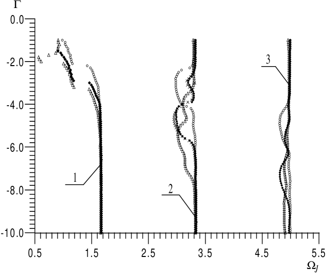
Figure 5: Voltage as function of magnetic field $\Gamma$ for $\alpha=0.3$, $L=5$ and different values of bias current: 1 - $\eta_{0}=0.5$, 2 - $\eta_{0}=1$, 3 - $\eta_{0}=1.5$; open circles - $x_{0}=0$, filled diamonds - $x_{0}=2.5$, open triangles - $x_{0}=4$; crosses - theory for $\eta_{0}=1$, $x_{0}=2.5$ (dimensionless units).

References

- (1) T. Nagatsuma, K. Enpuku, F. Irie, and K. Yoshida, J. Appl. Phys., 54, 3302 (1983); 56, 3284 (1984).
- (2) V. P. Koshelets and S. V. Shitov, Supercond. Sci. Technol., 13, R53 (2000).
- (3) V. P. Koshelets and J. Mygind, ”Flux Flow Oscillators For Superconducting Integrated Submm Wave Receivers”, Studies of High Temperature Superconductors, edited by A. V. Narlikar, NOVA Science Publishers, New York, vol. 39, pp. 213-244, (2001).
- (4) E. Joergensen, V. P. Koshelets, R. Monaco, J. Mygind, M. R. Samuelsen, and M. Salerno, Phys. Rev. Lett., 49, 1093 (1982).
- (5) V. P. Koshelets, A. Shchukin, I. L. Lapytskaya, and J. Mygind, Phys. Rev. B, 51, 6536 (1995).
- (6) V. P. Koshelets, S. V. Shitov, A. V. Shchukin, L. V. Filippenko, J. Mygind, and A. V. Ustinov, Phys. Rev. B, 56, 5572 (1997).
- (7) M. Cirillo, T. Doderer, S. G. Lachenmann, F. Santucci and N. Grønbech-Jensen, Phys. Rev. B, 56, 11889 (1997).
- (8) D. W. McLaughlin and A. C. Scott, Phys. Rev. A, 18, 1652 (1978).
- (9) I. O. Kulik, JETP Lett., 2, 84 (1965).
- (10) M. Cirillo, N. Grønbech-Jensen, M. R. Samuelsen, M. Salerno, G. Verona Rinati, Phys. Rev. B, 58, 12377 (1998).
- (11) M. Salerno and M. R. Samuelsen, Phys. Rev. B, 59, 14653 (1999).
- (12) M. Jaworski, Phys. Rev. B, 60, 7484 (1999).
- (13) Y. Zhang, Dynamics and Applications of Long Josephson Junctions, Ph.D. thesis, Chalmers University of Technology, Sweden, (1993).
- (14) V. P. Koshelets, A. B. Ermakov, P. N. Dmitriev, A. S. Sobolev, A. M. Baryshev, P. R. Wesselius and J. Mygind, Supercond. Sci. Technol., 14, 1 (2001).
- (15) A. L. Pankratov, Phys. Rev. B, 65, 054504-1 (2002).
- (16) V. P. Koshelets, P. N. Dmitriev, A. N. Mashentsev, A. S. Sobolev, V. V. Khodos, A. L. Pankratov, V. L. Vaks, A. M. Baryshev, P. R. Wesselius, and J. Mygind, Physica C, in press (2002).
- (17) K. K. Likharev, Dynamics of Josephson Junctions and Circuits (Gordon and Breach, New York, 1986).
- (18) A. Barone and G. Paternò, Physics and Applications of the Josephson Effect (J. Wiley, New York, 1982).