A Statistical Mechanics Model of Isotropic Turbulence Well-Defined within the Context of the $\epsilon$ Expansion

Abstract

A statistical mechanics model of isotropic turbulence that renormalizes the effects of turbulent stresses into a velocity-gradient-dependent random force term is introduced. The model is well-defined within the context of the renormalization group $\epsilon$ expansion, as the effective expansion parameter is $O(\epsilon)$. The Kolmogorov constant and $N$ parameter of turbulence are of order unity, in accord with experimental results. Nontrivial intermittency corrections to the single-time structure functions are calculated as a controlled expansion in $\epsilon$.

1 Introduction

Turbulence remains an outstanding problem in classical mechanics. Early on, several self-consistent or closure-based statistical models were introduced, with perhaps Kraichnan’s Direct Interaction Approximation the most well known [1]. Within the statistical mechanics literature, attention has focused upon the random force model that Dominicis and Martin [2] generalized from Forster, Nelson, and Stephen’s model of a randomly stirred equilibrium fluid [3]. This model has received quite a bit of attention, and its transport properties have been further examined by Yakhot and Orszag and Avellaneda and Majda and co-workers [4, 5, 6]. Various treatments, up to and including field-theoretic $\epsilon$ expansions, have been applied to the random force model of turbulence. As pointed out by Eyink, however, even the $\epsilon$ expansion does not lead to a controlled calculation in the random force model because the term representing the effects of high Reynolds numbers must be calculated to arbitrarily high order in perturbation theory, even for an $O(\epsilon)$ calculation [7]. More recently, a variety of novel renormalization group techniques has been applied to the problem of Navier-Stokes turbulence [8, 9, 10, 11].

The experimentally observed scaling behavior of turbulent energy dissipation, often called the Kolmogorov energy cascade, suggests that there may be a strong analogy between critical phenomena and turbulence. Indeed, the search for such an analogy motivated much of the field-theoretic work on fluid turbulence [12]. Just as there are wild fluctuations in particle density near a critical point, so to are there large fluctuations in the fluid velocity at high Reynolds number turbulence. This similarity suggests that the effects of turbulence may be modeled by a random, velocity-dependent force, just as the effects of critical fluctuations can be modeled by a random, density-dependent force in the standard $\phi^{4}$ model. While there are likely random forces that are independent of the fluid velocity in the context of turbulence, there are also very likely random forces that are velocity dependent. Thus, the turbulent force should really depend on the gradient of the velocity, as it is not simply large velocities that lead to turbulence, but rather regions of high gradient, such as walls or boundaries, that lead to turbulent behavior. Such boundary roughness is one mechanism for breaking the symmetry from laminar to turbulence fluid flow.

Indeed, random boundary roughness along the walls generates velocity-gradient-dependent forces in the bulk that are quenched in time. Moreover, in practical, engineering-type calculations, the turbulent forces are often related to velocity gradients by a constitutive relation that contains a “turbulent viscosity” parameter, the simplest of these relations being linear [13]. Following this line of reasoning, we introduce a new statistical mechanics model for turbulence that renormalizes the effect of turbulent stresses into a velocity-gradient-dependent term. This model will turn out to be well-defined within the $\epsilon$ expansion. That is, the renormalization group theory takes into account all physical effects of this model, consistently to order $\epsilon$. Due to its similarity with turbulent viscosity type models, this approach may lead to a closer connection with practical turbulence calculations.

We introduce our velocity-gradient-dependent random force model in Sec. 2. The problem is cast in the framework of time-dependent field theory in Sec. 3. Renormalization group flow equations are also calculated in this section, and three appendices provide details of the renormalization group calculations. The behavior of these flow equations in two and three dimensions, and the predictions for the Kolmogorov energy cascade, are described in Sec. 4. Nontrivial intermittency corrections to the single-time structure functions are calculated by an operator product expansion in Sec. 5. We conclude in Sec. 6.

2 Velocity-Gradient-Dependant Random Force Model

Our goal is to write a form of the Navier-Stokes equation that contains a random piece, the random piece representing the statistical effects of the turbulence. The Navier-Stokes equation with a random force is

$$\partial_{t}v_{i}+\sum_{k}\textstyle{\prod_{ik}}\sum_{j}v_{j}\partial_{j}v_{k}=\nu\nabla^{2}v_{i}+f_{i}\ ,$$ (1)

where $\nu=\mu/\rho$ is the kinematic viscosity, and $f_{i}=\sum_{k}\Pi_{ik}(F_{k}-\partial_{k}P)/\rho$ is the total body force on the fluid. The presence of the projection operator $\hat{\Pi}_{ik}({\bf k})=\delta_{ik}-k_{i}k_{k}/k^{2}$ in these formulas ensures that the incompressibility condition $\nabla\cdot{\bf v}=0$ is maintained [3]. The Fourier transform is defined by $\hat{f}({\bf k})=\int d{\bf x}f({\bf x})\exp(i{\bf k}\cdot{\bf x})$.

We choose the random force to depend on the gradient of the velocity:

$$f_{i}({\bf x},t)=-\gamma_{ijk}({\bf x})\partial_{j}v_{k}({\bf x},t)\ .$$ (2)

We assume that $\gamma_{ijk}$ is symmetric under exchange of $j$ and $k$, so that the force looks like a turbulent stress. We average over the statistics of this force using a field-theoretic representation of the Navier-Stokes equation. We choose the correlation function to be

$$\langle\hat{\gamma}_{ijk}({\bf k}_{1})\hat{\gamma}_{lmn}({\bf k}_{2})\rangle=(2\pi)^{d}\delta({\bf k}_{1}+{\bf k}_{2})|{\bf k}_{1}|^{-y}D_{ijk}^{lmn}\ ,$$ (3)

where

$$D_{ijk}^{lmn}=D_{\alpha}(\delta_{il}\delta_{jm}\delta_{kn}+\delta_{in}\delta_{jm}\delta_{kl}$$

$$+\delta_{il}\delta_{jn}\delta_{km}+\delta_{im}\delta_{jl}\delta_{kn}+\delta_{im}\delta_{jn}\delta_{kl}+\delta_{in}\delta_{jl}\delta_{km})$$

$$+D_{\beta}(\delta_{ij}\delta_{lm}\delta_{kn}+\delta_{ik}\delta_{jm}\delta_{ln}+\delta_{ik}\delta_{jn}\delta_{lm}+\delta_{ij}\delta_{km}\delta_{ln})\ .$$

(4)

Initially, we treat this as a mathematical problem, taking $y$ to be arbitrary. Later, we determine $y$ by requiring that the transport properties of turbulence are reproduced. This scaling form of the correlation function, Eq. (3), applies only in the inertial, Kolmogorov regime, for wavevectors below an upper cutoff related to the inverse of the dissipation length scale and above a lower cutoff related to the inverse of the so-called integral length scale. It is this Kolmogorov scaling regime that is of interest in the present work. Given the form of Eq. 2, the parameters $\sqrt{D}_{\alpha}$ and $\sqrt{D}_{\beta}$ can be viewed as modeling gradients of the turbulent viscosity.

3 Renormalization Group Calculations

We write the Navier-Stokes equation in field-theoretic form so that the renormalization group can be applied systematically within the $\epsilon$ expansion [14]. Within the field-theoretic formalism, any observable can be calculated. The average velocity, for example, is given by $v_{i}({\bf x},t)=\langle b_{i}({\bf x},t)\rangle$, where the average over the $b$ field is taken with respect to the weight $\exp(-S)$. Using Eqs. 1–4, we arrive at the following action:

$$S = \int_{\bf k}\int dt~{}\hat{\bar{b}}_{i}(-{\bf k},t)[\partial_{t}+\nu k^{2}+\delta(t)]\hat{b}_{i}({\bf k},t)$$

$$+i\lambda\int_{{\bf k}_{1}{\bf k}_{2}{\bf k}_{3}}\int dt~{}(2\pi)^{d}\delta({\bf k}_{1}+{\bf k}_{2}+{\bf k}_{3})$$

$$~{}~{}~{}~{}~{}~{}~{}~{}~{}~{}\times k_{1_{j}}\hat{\bar{b}}_{k}^{\perp}({\bf k}_{1},t)\hat{b}_{k}^{\perp}({\bf k}_{2},t)\hat{b}_{j}^{\perp}({\bf k}_{3},t)$$

$$+\frac{1}{2}\int_{{\bf k}_{1}{\bf k}_{2}{\bf k}_{3}{\bf k}_{4}}\int dt_{1}dt_{2}~{}(2\pi)^{d}\delta({\bf k}_{1}+{\bf k}_{2}+{\bf k}_{3}+{\bf k}_{4})$$

$$~{}~{}~{}~{}~{}~{}~{}~{}~{}~{}\times{{\bf k}_{2}}_{j}{{\bf k}_{4}}_{m}D_{ijk}^{lmn}|{\bf k}_{1}+{\bf k}_{2}|^{-y}$$

$$~{}~{}~{}~{}~{}~{}~{}~{}~{}~{}\times\hat{\bar{b}}_{i}^{\perp}({\bf k}_{1},t_{1})\hat{b}_{k}^{\perp}({\bf k}_{2},t_{1})\hat{\bar{b}}_{l}^{\perp}({\bf k}_{3},t_{2})\hat{b}_{n}^{\perp}({\bf k}_{4},t_{2})\ .$$

The notation $\int_{\bf k}$ stands for $\int d{\bf k}/(2\pi)^{d}$, the integrals over time are from $t=0$ to some large time $t=t_{f}$, and the summation convention is implied. This action is written in terms of the divergence-free part of the field, $\hat{b}_{i}^{\perp}({\bf k})=\sum_{k}\hat{\Pi}_{ik}({\bf k})\hat{b}_{k}({\bf k})$. We have used the Feynman gauge, adding in a curl-free component in the quadratic terms to make later calculations easier. Initially $\lambda=1$. We have used the replica trick [15] to incorporate the statistical disorder, but have suppressed these details since they do not enter in a one-loop calculation.

We now apply renormalization group theory to this action. It is important to note that the fields must all have zero average value before the renormalization group is applied [16, 17], otherwise it would not be correct to truncate perturbation theory at any finite order. If there were an average velocity, the action in (LABEL:5) would be different, containing a term of the form $-i{\bf k}\cdot\langle{\bf v}\rangle$ in the propagator. The vertices in the theory are shown in Fig. 1.

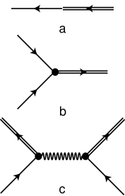
Figure 1: (a) Diagram representing the propagator. The arrow points in the direction of increasing time, and double lines represent the bar fields. (b) Convection vertex $\lambda$. (c) Disorder vertex $D_{\alpha}$ and $D_{\beta}$.

From power counting, the upper critical dimension for this theory is $d_{\rm c}=2+y$. Note that this upper critical dimension is exactly defined once the model is specified [14]. The deviation of the physical dimension from the upper critical dimension is parameterized by $\epsilon=d_{\rm c}-d$. We use the momentum shell procedure, where fields on a shell of differential width $\ln a=dl$ are integrated out, $\Lambda/a<k<\Lambda$. Note that the combination $dl$ invariably means a differential on $l$; in all other cases, the factor $d$ denotes the physical dimension. As usual, we rescale time by the dynamical exponent $t^{\prime}=a^{-z}t$ and distance by ${\bf k}_{\perp}^{\prime}=a{\bf k}_{\perp}$. The $b$ field is scaled as $\hat{b}^{\prime}({\bf k}^{\prime},t^{\prime})=a^{z-1-d+\alpha}\hat{b}({\bf k},t)$. To maintain dimensional consistency, so that the $b$ field scales as a velocity, one must set $\alpha=0$ [17]. To keep the time derivative in $S$ constant [18], the $\bar{b}$ field is scaled as $\hat{\bar{b}}^{\prime}({\bf k}^{\prime},t^{\prime})=a^{1-z-\alpha}\hat{\bar{b}}({\bf k},t)$. In the loop calculation, we make use of the relation for the reference system averages

$$\langle\hat{\bar{b}}_{i}^{\perp}({\bf k}_{1},t_{1})\hat{b}_{j}^{\perp}({\bf k}_{2},t_{2})\rangle_{0} = (2\pi)^{d}\delta({\bf k}_{1}+{\bf k}_{2})$$

$$\times\hat{\Pi}_{ij}({\bf k}_{2})\hat{G}_{0}({\bf k}_{2},t_{2}-t_{1})$$

where $\hat{G}_{0}({\bf k},t)=\exp[-\nu k^{2}t]\Theta(t)$, and $\Theta(t)=1$ if $t>0$ and 0 otherwise. Note that elimination of modes at one end of the spectrum by perturbation theory is the standard procedure in renormalization group theory [14]. Use of Eq. (LABEL:5aaa) does not imply that the system is somehow Gaussian, as the parameters within the renormalized theory are flowing. The critical properties of the Ising model at the non-Gaussian Wilson-Fisher fixed point, for example, are analyzed in exactly this way [14]. We make use of the rotational averages: $\langle k_{l}k_{u}\rangle_{\Omega}=\delta_{lu}k^{2}/d$, $\langle k_{l}k_{m}k_{s}k_{u}\rangle_{\Omega}=(\delta_{lm}\delta_{us}+\delta_{lu}\delta_{ms}+\delta_{ls}\delta_{mu})k^{4}/[d(d+2)]$, and $\langle k_{l}k_{m}k_{n}k_{s}k_{t}k_{u}\rangle_{\Omega}=M_{lmn}^{stu}k^{6}/[d(d+2)(d+4)]$, where the function $M_{lmn}^{stu}$ is equal to all possible couplings of pairs of the arguments:

$$M_{lmn}^{stu} = \delta_{lt}\delta_{ms}\delta_{nu}+\delta_{lt}\delta_{mn}\delta_{su}+\delta_{lt}\delta_{mu}\delta_{ns}$$ (7)

$$+ \delta_{lm}\delta_{ts}\delta_{nu}+\delta_{lm}\delta_{nt}\delta_{su}+\delta_{lm}\delta_{tu}\delta_{ns}$$

$$+ \delta_{ls}\delta_{mt}\delta_{nu}+\delta_{ls}\delta_{mn}\delta_{tu}+\delta_{ls}\delta_{mu}\delta_{nt}$$

$$+ \delta_{ln}\delta_{mt}\delta_{su}+\delta_{ln}\delta_{ms}\delta_{tu}+\delta_{ln}\delta_{mu}\delta_{st}$$

$$+ \delta_{lu}\delta_{mt}\delta_{ns}+\delta_{lu}\delta_{mn}\delta_{st}+\delta_{lu}\delta_{ms}\delta_{nt}\ .$$

The one loop contributions are shown in Fig. 2.

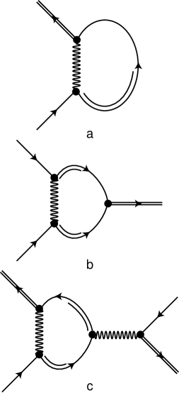
Figure 2: One-loop diagrams: (a) self-energy diagrams contributing to $\nu$, (b) vertex diagrams contributing to $\lambda$, and (c) vertex diagrams contributing to $D_{\alpha}$ and $D_{\beta}$.

There are 13 diagrams of the form Fig. 2a, detailed calculation of which is described in Appendix A. There are 13 similar diagrams of the form Fig. 2b, detailed calculation of which is described in Appendix B. Finally, there are 100 diagrams of the form Fig. 2c, and a detailed discussion of them is given in Appendix C. These last diagrams require some care in their calculation, as they contribute to the complex tensor structure of $D_{ijk}^{lmn}$ in Eq. (LABEL:5). These last diagrams make contributions in the form

$${{\bf k}_{2}}_{j}{{\bf k}_{4}}_{v}\hat{\bar{b}}_{i}^{\perp}({\bf k}_{1},t_{1})\hat{b}_{k}^{\perp}({\bf k}_{2},t_{1})\hat{\bar{b}}_{r}^{\perp}({\bf k}_{3},t_{2})\hat{b}_{w}^{\perp}({\bf k}_{4},t_{2})$$

$$~{}~{}~{}~{}~{}~{}~{}~{}~{}~{}\times M_{lmn}^{stu}D_{ijk}^{lmn}D_{rst}^{uvw}\ .$$ (8)

There are 15 terms of the form Fig. 2c when the sums over $l,m,n$ and $s,t,u$ are taken. Each of these terms corresponds to one of the 15 terms in Eq. (7), and each gives a contribution that is exactly of the form in Eq. (LABEL:5). The theory is, therefore, self-consistent in that no terms are generated at this order that are not of the original form, and the symmetry of the original theory is maintained.

The flow equations that result from the one-loop calculation are

$$\frac{d\ln\nu}{dl} = z-2+[(d^{2}+2d-2)D_{\alpha}+(d-2)D_{\beta}]$$

$$~{}~{}~{}~{}~{}~{}~{}~{}~{}~{}\times\frac{yK_{d}}{\nu^{2}d(d+2)}\Lambda^{-\epsilon}$$

$$\frac{d\ln\lambda}{dl} = -\alpha-[(d^{2}+2d-2)D_{\alpha}+(d-2)D_{\beta}]$$

$$~{}~{}~{}~{}~{}~{}~{}~{}~{}~{}\times\frac{K_{d}}{\nu^{2}d(d+2)}\Lambda^{-\epsilon}$$

$$\frac{d\ln D_{\alpha}}{dl} = 2z-4+\epsilon-[2D_{\alpha}+4D_{\beta}]$$

$$~{}~{}~{}~{}~{}~{}~{}~{}~{}~{}\times\frac{2K_{d}(d^{2}+2d-2)}{\nu^{2}d(d+2)(d+4)}\Lambda^{-\epsilon}$$

$$\frac{d\ln D_{\beta}}{dl} = 2z-4+\epsilon-[2(d^{2}+2d-2)D_{\alpha}^{2}/D_{\beta}$$ (9)

$$~{}~{}~{}+(d^{3}+6d^{2}-8)D_{\alpha}+(d^{2}+2d-8)D_{\beta}]$$

$$~{}~{}~{}~{}~{}~{}~{}~{}~{}~{}\times\frac{2K_{d}}{\nu^{2}d(d+2)(d+4)}\Lambda^{-\epsilon}\ .$$

The constant $K_{d}=S_{d}/(2\pi)^{d}$, and $S_{d}=2\pi^{d/2}/\Gamma(d/2)$. In solving these equations, we set $\alpha=0$ for dimensional consistency. In the standard model of turbulence [2], terms higher order in $\lambda(l)$ must be kept in the flow equations. In the present model, $\lambda(l)$ flows to zero rapidly, and higher order do not contribute at this level.

4 Results and Discussion

In two dimensions, both $D_{\alpha}$ and $D_{\beta}$ are relevant. We find a fixed point of $D_{\alpha}^{*}=D_{\beta}^{*}=2\epsilon\nu^{2}\Lambda^{\epsilon}/[3K_{2}(1+y)]$. The dynamical exponent is given by $z=2-y\epsilon/[2(1+y)]$. The Reynolds number term scales as $\lambda(l)=\lambda_{0}e^{-\epsilon l/[2(1+y)]}$.

In greater than two dimensions, $D_{\beta}$ reaches a fixed point, but $D_{\alpha}$ flows to zero. We find

$$D_{\beta}^{*} = \frac{d(d+2)\nu^{2}\Lambda^{\epsilon}}{2(1+y)(d-2)K_{d}}\epsilon$$

$$z = 2-\frac{y\epsilon}{2(1+y)}$$

$$\lambda(l) = \lambda_{0}e^{-\epsilon l/[2(1+y)]}\ .$$ (10)

Interestingly, the dynamical exponent is the same in two and greater dimensions, as is the decay of $\lambda(l)$.

A particularly beautiful feature of this theory is that $\lambda(l)$ decays exponentially to zero. This property is what makes the theory well defined within the epsilon expansion. If $\lambda(l)$ had stayed at unity, the vertex in Fig. 1b could be inserted arbitrarily many times in the loop expansion, and terminating the expansion at any finite order would not be justified by any small parameter. The present calculation, on the other hand, is a controlled expansion in $\epsilon$ and $\lambda(l)$. Note that the quenched random forces, which mimic the effects of, say, wall roughness, break statistical Galilean invariance, and this allows $\lambda(l)$ to flow, in contrast to the conventional model with random forces delta-correlated in time. Indeed, our explicit calculation shows that $\lambda(l)$ decays exponentially to zero.

We now turn to a calculation of the energy spectrum, defined by [19]

$$E({\bf k})=\frac{(d-1)}{2}K_{d}k^{d-1}\hat{C}_{11}({\bf k})\ ,$$ (11)

where the velocity-velocity correlation function is given in the field-theoretic language as

$$(2\pi)^{d}\delta({\bf k}_{1}+{\bf k}_{2})\hat{\Pi}_{ij}({\bf k}_{1})\hat{C}_{ij}({\bf k}_{1})=\langle\hat{b}_{i}^{\perp}({\bf k}_{1},t)\hat{b}_{j}^{\perp}({\bf k}_{2},t)\rangle\ .$$ (12)

Under the scaling of time and space that occurs within the renormalization group calculation, this correlation function scales as

$$\hat{C}_{ij}({\bf k}) = \frac{a^{2(d+1-z-\alpha)}}{a^{d}}\frac{\langle{\hat{b}_{i}^{\perp}}{{}^{\prime}}({\bf k}_{1}^{\prime},t^{\prime}){\hat{b}_{j}^{\perp}}{{}^{\prime}}({\bf k}_{2}^{\prime},t^{\prime})\rangle}{(2\pi)^{d}\delta({\bf k}_{1}^{\prime}+{\bf k}_{2}^{\prime})\hat{\Pi}_{ij}({\bf k}_{1}^{\prime})}$$ (13)

$$= a^{d+2-2z-2\alpha}\hat{C}^{\prime}_{ij}({\bf k}^{\prime})\ .$$

Making the assumption that $\hat{C}_{ij}({\bf k})\sim({\rm const})k^{-\delta}$, we find from Eq. 13 that $\delta=d+2-2z-2\alpha$. The energy spectrum, therefore, scales as

$$E({\bf k})\sim({\rm const})k^{2z-3+2\alpha}\ .$$ (14)

For any isotropic statistical theory of turbulence, then, the dimensional consistency condition of $\alpha=0$ enforces a relation between the dynamical exponent and the exponent of the energy cascade. In particular, the Richardson separation law implies $z=2/3$, and this result is equivalent to enforcing the Kolmogorov energy cascade: $E({\bf k})\sim({\rm const})k^{-5/3}$. The relation $z=2/3$ implies $y=3.44152$ in two dimensions and $y=4.28849$ in three dimensions.

To calculate the Kolmogorov constant $C_{\rm K}$ we introduce a source of randomness into the model:

$$\delta S=-\frac{D}{2}\sum_{i}\int dt\int_{\bf k}\hat{c}(k)\hat{\bar{b}}_{i}^{\perp}(-{\bf k},t)\hat{\bar{b}}_{i}^{\perp}({\bf k},t)\ .$$ (15)

In the range for which scaling occurs, we set $\hat{c}(k)\sim k^{3z-2-d}$. For later convenience, we also require that $\lim_{r\to 0}c(r)=1$. The randomness expressed in this source term drives the model away from the trivial solution $v_{i}({\bf x},t)\equiv 0$. Note that the randomness parameter scales as $D(l)\equiv D$. This randomness parameter does not contribute to $\nu$ since $\lambda(l)$ flows to zero, and nothing contributes to $D(l)$ at one loop. Since $D(l)$ contributes to physical properties at higher loops only through $\lambda(l)$, $D_{\alpha}(l)$, and $D_{\beta}(l)$, all of which are small, the effects of $D$ are controlled within the $\epsilon$ expansion. Using the matching Eq. 13, the correlation function is given by $\hat{C}_{ij}({\bf k})=[D\Lambda^{z-2}/(2\nu)]k^{-\delta}$. For fully-developed isotropic turbulence $z=2/3$, and using the notation [4]

$$E({\bf k})\sim C_{\rm K}\varepsilon^{2/3}k^{-5/3}\ ,$$ (16)

we find $C_{\rm K}\varepsilon^{2/3}=(d-1)K_{d}D\Lambda^{-4/3}/(4\nu)$. Similarly, the wavevector-dependent viscosity considered in the fluid mechanics literature [4] is given by $\nu({\bf k})=\nu\Lambda^{4/3}k^{-4/3}$. Using the notation [4]

$$\nu({\bf k})\sim N\varepsilon^{1/3}k^{-4/3}\ ,$$ (17)

we find $N\varepsilon^{1/3}=\nu\Lambda^{4/3}$. The energy dissipation rate is given by

$$\varepsilon=\int_{0}^{\Lambda}dk~{}2\nu k^{2}E(k)\ .$$ (18)

Using Eqs. (16) and (18), we find $\varepsilon=(27/8)\nu^{3}C_{\rm K}^{3}\Lambda^{4}$. Finally, to complete the matching we assume that the wavevector cutoff is one-half the Kolmogorov dissipation number, $2\Lambda=k_{d}\equiv(\varepsilon/\nu^{3})^{1/4}$ [20]. Putting these relations together in three dimensions, we find

$$\varepsilon = 0.0380D$$

$$C_{\rm K} = 1.68$$

$$N = 0.397\ .$$ (19)

Note that field theory cannot calculate non-universal parameters such as these with precision, as these results depend on the assumption in Eq. (18) and the relation between $\Lambda$ and $k_{d}$. A more detailed matching calculation of these values using the model of turbulence in Eqs. (3) and (15) to refine the matching calculation would be of interest.

5 Intermittency

We here address the issue of intermittency in our model. That is, we seek to determine the scaling of the single-time structure function

$$S_{2n}(r)=\langle\left[|{\bf b}^{\perp}({\bf x}+{\bf r})-{\bf b}^{\perp}({\bf x})|^{2}\right]^{n}\rangle\sim({\rm const})r^{\zeta_{2n}}\ .$$ (20)

From simple dimensional analysis, we find $\zeta_{2n}=nz$. From explicit calculation for our model, we find an exponent that differs from this value. This difference is referred to in the fluid mechanics literature as intermittency. That $\zeta_{2n}\neq nz$ is an expression of the non-Gaussian nature of the fixed point identified in our model and of the divergence of the single-time structure functions in the limit of an infinite integral length scale.

We use the same arguments about scaling of space and time as in Eq. 13 to express the original correlation function in terms of the renormalized correlation function:

$$S_{2n}(r)\sim e^{n(2-2z)l}S_{2n}(r(l);l)\ .$$ (21)

Here $r=\exp(l)r(l)$. This equation is applied until $r(l)$ is of the order of the dissipation length scale $r(l^{*})=2\pi/\Lambda\equiv h$. At this length scale, we then match the correlation function to a perturbation theory result:

$$S_{2n}(r(l^{*});l^{*}) \propto \left[\frac{h^{2}}{2\nu}c(h;l^{*})\right]^{n}$$ (22)

$$= \left(\frac{h^{2}}{2\nu}\right)^{n}e^{(3z-2)nl^{*}}c^{n}(h)$$

$$= \left(\frac{h^{2}}{2\nu}\right)^{n}e^{(3z-2)nl^{*}}\ ,$$

where we have used the scaling of the small-$r$ behavior of the $c(r)$ function in Eq. 15 and have used $\lim_{h\to 0}c(h)=1$. Combining Eqs. 21 and 22 we find

$$S_{2n}(r)\sim({\rm const})r^{nz}f_{n}(r/L)\ .$$ (23)

We have here introduced the fact that traditional renormalization group arguments can determine asymptotic behavior only up to a scaling function of the ratio $r/L$, where $L$ is the macroscopic size of the system. This is because $r$ and $L$ are scaled by the same factor in the renormalization group analysis, and so no dependence on the ratio $r/L$ is detectable. For turbulence, $h$ is the dissipation length scale, and $L$ is the integral length scale. In many applications of renormalization group theory to condensed matter systems, the scaling function $f_{n}(r/L)\sim({\rm const})$ as $L\to\infty$, and so it does not play a role. In our case, on the other hand, the scaling function gives the corrections to intermittency.

To determine the function $f_{n}$ we use the operator product expansion [14, 21, 22]. A similar strategy has proven successful in the study of turbulent transport of passive scalars [23]. The operator product expansion states that

$$\langle F({\bf x}_{1})F({\bf x}_{2})\rangle\sim\sum_{\alpha}c_{\alpha}(|{\bf x}_{1}-{\bf x}_{2}|)\langle F_{\alpha}^{R}({\bf x})\rangle\ .$$ (24)

Here the ${\bf x}=({\bf x}_{1}+{\bf x}_{2})/2$, and $F_{\alpha}^{R}$ is the set of all renormalized operators that are generated by the renormalization group flow of $F$. Equation 24 is nothing more than a Taylor series expansion, where both the bare terms in the Taylor series and those terms that are generated by the renormalization flow are included. In our particular case, instead of a pair of operators, we have $S_{2n}$, which is a product of $2n$ factors on the left hand side of this equation. The important point about this expansion is that the functions $c_{\alpha}(r)$ are finite and exhibit no dependence on the system size $L$. Any possible system size dependence of this expansion, therefore, is contained within $\langle F_{\alpha}^{R}({\bf x})\rangle$. By comparison to Eq. 23, we see that the scaling function $f_{n}$ is thus determined by the behavior of these renormalized operators. We first determine the scaling of the renormalized operators:

$$\langle F_{\alpha}^{R}\rangle=e^{\Delta_{\alpha}l^{*}}\langle F_{\alpha}^{R}(l^{*})\rangle\ .$$ (25)

We follow the renormalization flows until $L(l^{*})=\exp(-l^{*})L=r$, a criterion that automatically ensures the functional form specified in Eq. 23. We thus conclude that

$$\langle F_{\alpha}^{R}\rangle=\left(\frac{r}{L}\right)^{-\Delta_{\alpha}}\langle F_{\alpha}^{R}(l^{*})\rangle\ .$$ (26)

In fact, we determine the scaling of these operator averages by using the generating functional $\delta S=-A_{\alpha}\int dt\int d^{d}{\bf x}F_{\alpha}^{R}$. We will find

$$A_{\alpha}(l)\sim e^{(z+d-2nz+\gamma_{\alpha})l}A_{\alpha}(0)\ .$$ (27)

In terms of $A_{\alpha}$ and the partition function $Z$, the operator average is given by

$$\int dt\int d^{d}{\bf x}\langle F_{\alpha}^{R}\rangle=\left.\frac{d\ln Z}{dA_{\alpha}(0)}\right|_{A_{\alpha}(0)=0}\ .$$ (28)

This equation makes clear why Eq. 25 has the form that it does and identifies $\Delta_{\alpha}=-2nz+\gamma_{\alpha}$. The value of $\gamma_{\alpha}$ will be determined by a nontrivial fixed point of the renormalization group flow equations for $A_{\alpha}$. Combining Eqs. 26 and 27, we find

$$\langle F_{\alpha}^{R}\rangle\sim\left(\frac{r}{L}\right)^{2nz-\gamma_{\alpha}}\langle F_{\alpha}^{R}(l^{*})\rangle\ .$$ (29)

The function $\langle F_{\alpha}^{R}(l^{*})\rangle$ is determined by matching exactly as in Eq.  22. We, thus, find that

$$\langle F_{\alpha}^{R}\rangle \sim \left(\frac{r}{L}\right)^{2nz-\gamma_{\alpha}}\left(\frac{r}{L}\right)^{(2-3z)n}$$ (30)

$$= \left(\frac{r}{L}\right)^{n(2-z)-\gamma_{\alpha}}\ .$$

To make use of this result of the operator product expansion, it remains only to calculate the value of $\gamma_{\alpha}$. Once we have this value, we find the scaling function to be

$$f_{2n}(r/L)\sim\left(\frac{r}{L}\right)^{n(2-z)-\gamma_{\alpha}}{\rm as~{}}L{\rm~{}to~{}}\infty\ .$$ (31)

In fact, the operator $S_{2n}$ will generate several new operators $F_{\alpha}$ in the expansion of Eq. 24. The appropriate value of $\gamma_{\alpha}$ to use in Eq. 31 is the largest one. These generated operators may mix upon the renormalization, in which case the appropriate value of $\gamma_{\alpha}$ is the largest eigenvalue of the flow equation matrix.

We first determine the scaling function $f_{1}$. We limit consideration to the case $d>2$, where $D_{\alpha}^{*}=0$. The correlation function $S_{2n}$ is given in a Taylor series as $S_{2n}(r)\sim[r^{2}\partial_{x}b_{i}\partial_{x}b_{i}]^{n}$. This will generate the symmetrized operator $F=[\partial_{j}b_{i}\partial_{j}b_{i}+\partial_{i}b_{j}\partial_{j}b_{i}]^{n}$, which we consider.

For the case $n=1$, we consider the generating functional

$$\delta S_{II} = -\int dt\int_{{\bf k}_{1}{\bf k}_{2}}\bigg{[}A^{(1)}{\bf k}_{1}\cdot{\bf k}_{2}\hat{b}^{\perp}({\bf k}_{1},t)\cdot\hat{b}^{\perp}({\bf k}_{2},t)$$ (32)

$$+A^{(0)}{\bf k}_{1}\cdot\hat{b}^{\perp}({\bf k}_{2},t){\bf k}_{2}\cdot\hat{b}^{\perp}({\bf k}_{1},t)\bigg{]}\ .$$

We find

$$\frac{dA^{(i)}}{dl}=(z+d-2z)A^{(i)}+\frac{2(d-1)g}{d}A^{(1)}\ ,$$ (33)

where $g=D_{\beta}K_{d}/(\nu^{2}\Lambda^{\epsilon})$. We, thus, identify $\gamma_{1}=2(d-1)g^{*}/d$. Using Eq. 10 we find in three dimensions $z=2-\epsilon/4+O(\epsilon^{2})$ and $g^{*}=15\epsilon/4+O(\epsilon^{2})$ and conclude from Eqs. 23 and 31 that

$$S_{2}(r) \sim ({\rm const})r^{z}\left(\frac{r}{L}\right)^{2-z-\gamma_{1}}$$ (34)

$$= ({\rm const})r^{2-\epsilon/4}\left(\frac{r}{L}\right)^{\epsilon/4-5\epsilon}\ .$$

We now determine the scaling function $f_{2}$. We start with the symmetrized generating functional

$$\delta S^{(2)} = -\int dt\int_{{\bf k}_{1}{\bf k}_{2}{\bf k}_{3}{\bf k}_{4}}\hat{b}^{\perp}({\bf k}_{1},t)\cdot\hat{b}^{\perp}({\bf k}_{2},t)$$ (35)

$$\times\hat{b}^{\perp}({\bf k}_{3},t)\cdot\hat{b}^{\perp}({\bf k}_{4},t)\bigg{[}A_{1}^{(2)}{\bf k}_{1}\cdot{\bf k}_{2}{\bf k}_{3}\cdot{\bf k}_{4}$$

$$+A_{2}^{(2)}({\bf k}_{1}\cdot{\bf k}_{3}{\bf k}_{2}\cdot{\bf k}_{4}+{\bf k}_{1}\cdot{\bf k}_{4}{\bf k}_{2}\cdot{\bf k}_{3})\bigg{]}\ .$$

This term generates two additional generating functionals:

$$\delta S^{(1)} = -\int dt\int_{{\bf k}_{1}{\bf k}_{2}{\bf k}_{3}{\bf k}_{4}}\hat{b}^{\perp}({\bf k}_{1},t)\cdot\hat{b}^{\perp}({\bf k}_{2},t)$$ (36)

$$\times\bigg{[}A_{1}^{(1)}{\bf k}_{1}\cdot{\bf k}_{2}{\bf k}_{4}\cdot\hat{b}^{\perp}({\bf k}_{3},t){\bf k}_{3}\cdot\hat{b}^{\perp}({\bf k}_{4},t)$$

$$+A_{2}^{(1)}\bigg{(}{\bf k}_{1}\cdot{\bf k}_{3}{\bf k}_{4}\cdot\hat{b}^{\perp}({\bf k}_{3},t){\bf k}_{2}\cdot\hat{b}^{\perp}({\bf k}_{4},t)$$

$$+{\bf k}_{1}\cdot{\bf k}_{4}{\bf k}_{2}\cdot\hat{b}^{\perp}({\bf k}_{3},t){\bf k}_{3}\cdot\hat{b}^{\perp}({\bf k}_{4},t)$$

$$+{\bf k}_{2}\cdot{\bf k}_{3}{\bf k}_{4}\cdot\hat{b}^{\perp}({\bf k}_{3},t){\bf k}_{1}\cdot\hat{b}^{\perp}({\bf k}_{4},t)$$

$$+{\bf k}_{2}\cdot{\bf k}_{4}{\bf k}_{1}\cdot\hat{b}^{\perp}({\bf k}_{3},t){\bf k}_{3}\cdot\hat{b}^{\perp}({\bf k}_{4},t)\bigg{)}$$

$$+A_{3}^{(1)}\bigg{(}{\bf k}_{3}\cdot{\bf k}_{4}{\bf k}_{1}\cdot\hat{b}^{\perp}({\bf k}_{3},t){\bf k}_{2}\cdot\hat{b}^{\perp}({\bf k}_{4},t)$$

$$+{\bf k}_{3}\cdot{\bf k}_{4}{\bf k}_{2}\cdot\hat{b}^{\perp}({\bf k}_{3},t){\bf k}_{1}\cdot\hat{b}^{\perp}({\bf k}_{4},t)\bigg{)}\bigg{]}$$

and

$$\delta S^{(0)} = -\int dt\int_{{\bf k}_{1}{\bf k}_{2}{\bf k}_{3}{\bf k}_{4}}\hat{b}_{i}^{\perp}({\bf k}_{1},t)\hat{b}_{j}^{\perp}({\bf k}_{2},t)\hat{b}_{k}^{\perp}({\bf k}_{3},t)\hat{b}_{l}^{\perp}({\bf k}_{4},t)$$ (37)

$$\times\bigg{[}A_{1}^{(0)}{{\bf k}_{1}}_{j}{{\bf k}_{2}}_{i}{{\bf k}_{3}}_{l}{{\bf k}_{4}}_{k}$$

$$+A_{2}^{(0)}\bigg{(}{{\bf k}_{1}}_{j}{{\bf k}_{2}}_{l}{{\bf k}_{3}}_{i}{{\bf k}_{4}}_{k}+{{\bf k}_{1}}_{j}{{\bf k}_{2}}_{k}{{\bf k}_{3}}_{l}{{\bf k}_{4}}_{i}$$

$$+{{\bf k}_{1}}_{l}{{\bf k}_{2}}_{i}{{\bf k}_{3}}_{j}{{\bf k}_{4}}_{k}+{{\bf k}_{1}}_{k}{{\bf k}_{2}}_{i}{{\bf k}_{3}}_{l}{{\bf k}_{4}}_{j}\bigg{)}$$

$$+A_{3}^{(0)}\bigg{(}{{\bf k}_{1}}_{k}{{\bf k}_{2}}_{l}{{\bf k}_{3}}_{i}{{\bf k}_{4}}_{j}+{{\bf k}_{1}}_{k}{{\bf k}_{2}}_{l}{{\bf k}_{3}}_{j}{{\bf k}_{4}}_{i}$$

$$+{{\bf k}_{1}}_{l}{{\bf k}_{2}}_{k}{{\bf k}_{3}}_{i}{{\bf k}_{4}}_{j}+{{\bf k}_{1}}_{l}{{\bf k}_{2}}_{k}{{\bf k}_{3}}_{j}{{\bf k}_{4}}_{i}\bigg{)}\bigg{]}$$

We will find $A_{2}^{(1)}(l)=A_{3}^{(1)}(l)$. Although we have included $A_{3}^{(0)}$ for generality, we will find that this term is not generated, and $A_{3}^{(0)}(l)=0$.

A lengthy calculation shows that

$$\frac{d{\bf A}}{dl}=(z+d-4z)I{\bf A}+\frac{g}{d(d+2)(d+4)}M{\bf A}$$ (38)

where the vector ${\bf A}=(A_{1}^{(2)},A_{2}^{(2)},A_{1}^{(1)},A_{2}^{(1)},A_{3}^{(1)},A_{1}^{(0)},A_{2}^{(0)})$, and the matrix $M$ is given in Table 1.

Table 1: The matrix $M$ in the calculation of the intermittency exponent $\zeta_{4}$ via Eq. 38.

$$M=\left(\begin{array}[]{ccccccc}4(d^{3}+5d^{2}+2d-6)&8(d+3)^{2}&8&16&4(d^{2}+6d+10)&8&16\\ 2(d+2)^{2}&2(d^{3}+5d^{2}-12)&-4(d+2)&-8(d+2)&d^{3}+4d^{2}-8d-24&2(d+2)^{2}&4(d+2)^{2}\\ 4(d^{3}+5d^{2}+2d-4)&8(d^{2}+6d+10)&2(d^{3}+5d^{2}+2d)&8(d^{2}+6d+12)&4(d^{2}+6d+12)&16&32\\ 2d(d+2)&2(d^{3}+5d^{2}-2d-16)&2d(d+2)&2(d^{3}+5d^{2}-6d-24)&d^{3}+4d^{2}-12d-32&2d(d+2)&4d(d+2)\\ 2d(d+2)&2(d^{3}+5d^{2}-2d-16)&2d(d+2)&2(d^{3}+5d^{2}-6d-24)&d^{3}+4d^{2}-12d-32&2d(d+2)&4d(d+2)\\ 8&8&2(d^{3}+5d^{2}+2d-4)&8(d^{2}+6d+10)&8&8&16\\ -2(d+2)&-2(d+2)&(d+2)^{2}&d^{3}+5d^{2}-2d-16&-2(d+2)&-2(d+2)&-4(d+2)\end{array}\right)$$

We diagonalize the matrix $M$, finding the eigenvalues $(0,0,0,0,d^{3}+4d^{2}-4d-16,2(d^{3}+5d^{2}+2d-8),4(d^{3}+7d^{2}+6d))$. The largest eigenvalue is the last one for all $d$. In three dimensions we identify $\gamma_{2}=432g^{*}/105$. Using Eqs.  23 and 31 we find that

$$S_{4}(r)\sim({\rm const})r^{4-\epsilon/2}\left(\frac{r}{L}\right)^{\epsilon/2-108\epsilon/7}\ .$$ (40)

We have, therefore, derived the intermittency corrections to dimensional analysis for the present model. The corrections are calculated in a controlled fashion and are proportional to $\epsilon$. The coefficients of the correction are not small, and for finite $\epsilon$, higher order terms in the expansion are required for an accurate estimation of the effects of intermittency.

One might wonder whether there are any corrections to the Kolmogorov energy cascade, Eq.  14, that arise from the operator product expansion. More generally, are there any corrections to $\langle[b_{i}^{\perp}({\bf x},t)b_{i}^{\perp}({\bf x},t)]^{n}\rangle$? There are no such corrections. This type of operator flows under the renormalization group only to operators with more derivatives, such as $\partial_{l}b_{j}^{\perp}\partial_{m}b_{k}^{\perp}(b_{i}^{\perp}b_{i}^{\perp})^{n-1}$. These operators are less relevant than the original operator, and so they make no contribution to the scaling at leading order. In the language of Eq. 24, $F_{\alpha}^{R}\equiv 1$, and the scaling function $f_{n}(r/L)\sim({\rm const})$ as $L\to\infty$.

6 Conclusion

An alternative, simpler model would have been to take the turbulent forces to be proportional to the velocity, rather than the velocity gradient. The simplest model, moreover, would take the forces to be white noise in time and uncorrelated in each of the spatial dimensions. For this model to be nontrivial, a mean fluid flow must be introduced [17]. Interestingly, when this is done for forces that are random in time as well as space, the resulting theory has the same flow equations as the traditional random force model of turbulence [2, 3]. Also of interest to note is that a theory with velocity-gradient-dependent random forces that are white noise in time would have no renormalization of any parameter, as the diagrams of Fig. 2 would all vanish due to the causality of the bare propagator, Eq. (LABEL:5aaa).

The scaling of the Kolmogorov energy cascade is determined once the value of the dynamical exponent is fixed, i.e. $z=2/3$ for isotropic turbulence. In random force models such as the present one, the scaling of the energy cascade simply serves to fix the correlation function of the random forcing. The predictive power of models such as these lie in their ability to provide nontrivial predictions of the intermittency corrections. In the present model, we are able to provide these corrections as a systematic expansion in $\epsilon$.

In summary, we have introduced a new statistical mechanics model for isotropic turbulence. This model makes use of a random, velocity-gradient-dependent force. This model is both consistent with practical, engineering-type calculations and well-defined within the renormalization group $\epsilon$ expansion. This model makes stronger the analogy between turbulence and critical phenomena.

Owing to the irrelevance of the convection terms at the fixed point, our results may alternatively be viewed as an analysis of transport in a new class of random media.

Appendix A: One-Loop contributions to $\nu$

We here show how the diagrams of Fig. 2a contribute to the propagator, Fig. 1a. Each of the terms is associated with one of the $D_{ijk}^{lmn}$ terms in Eq. (LABEL:5). In the calculation of the averages on the shell, there are five terms associated with $D_{\alpha}$ and three associated with $D_{\beta}$, as the last two terms associated with $D_{\alpha}$ are identical, and the last two terms associated with $D_{\beta}$ are also identical. The first term, associated with $D_{\alpha}$, is

$$I_{1} = 2\times\frac{D_{\alpha}}{2}\int dt_{1}dt_{2}\int_{{\bf k}_{1}{\bf k}_{2}{\bf k}_{3}{\bf k}_{4}}$$ (41)

$$\times(2\pi)^{d}\delta({\bf k}_{1}+{\bf k}_{2}+{\bf k}_{3}+{\bf k}_{4})|{\bf k}_{1}+{\bf k}_{2}|^{-y}$$

$$\times\Theta(t_{1}-t_{2})(2\pi)^{d}\delta({\bf k}_{2}+{\bf k}_{3})e^{-\nu k_{2}^{2}(t_{1}-t_{2})}$$

$$\times\left\{{\bf k}_{2}\cdot{\bf k}_{4}\hat{\bar{b}}_{i}^{\perp}({\bf k}_{1},t_{1})\hat{b}_{j}^{\perp}({\bf k}_{4},t_{2})\hat{\Pi}_{ij}({\bf k}_{2})\right\}$$

$$= \frac{K_{d}}{\nu^{2}}\left[D_{\alpha}\frac{y(d+1)}{d(d+2)}\right]\int_{\Lambda/a}^{\Lambda}dqq^{d-y-3}$$

$$\times\int dt\int_{\bf k}\nu k^{2}\hat{\bar{b}}_{i}^{\perp}(-{\bf k},t)\hat{b}_{i}^{\perp}({\bf k},t)$$

For the remaining contributions, we list the symmetry factor, terms in braces in the integrand of Eq. (41) that change, and the final contribution in brackets that change. The contributions are shown in Table 2, where the dependence of the fields upon time has been suppressed. The term $e^{-\nu k_{i}^{2}(t_{1}-t_{2})}$, which has the same momentum argument as the $\hat{\Pi}({\bf k}_{i})$ term, has been suppressed. The delta function is also suppressed. Summing all these contributions to $\nu$, we get the first flow equation of Eq. (9).

Table 2: Terms in the contributions from Fig. 2a, via Eq. 41.

Integral	Symmetry	Integrand	Result
$I_{1}$	2	$\left\{{k}_{2_{l}}{k}_{4_{l}}\hat{\bar{b}}_{i}^{\perp}({\bf k}_{1})\hat{b}_{j}^{\perp}({\bf k}_{4})\hat{\Pi}_{ij}({\bf k}_{2})\right\}$	$\left[D_{\alpha}\frac{y(d+1)}{d(d+2)}\right]$
$I_{2}$	2	$\left\{{k}_{2_{l}}{k}_{4_{l}}\hat{\bar{b}}_{i}^{\perp}({\bf k}_{1})\hat{b}_{i}^{\perp}({\bf k}_{4})\hat{\Pi}_{jj}({\bf k}_{2})\right\}$	$\left[D_{\alpha}\frac{y(d-1)}{d}\right]$
$I_{3}^{a}$	1	$\left\{{k}_{2_{i}}{k}_{4_{j}}\hat{\bar{b}}_{k}^{\perp}({\bf k}_{1})\hat{b}_{i}^{\perp}({\bf k}_{4})\hat{\Pi}_{jk}({\bf k}_{2})\right\}$	$\left[-\frac{D_{\alpha}}{2}\frac{y}{d(d+2)}\right]$
$I_{3}^{b}$	1	$\left\{{k}_{2_{i}}{k}_{4_{j}}\hat{\bar{b}}_{k}^{\perp}({\bf k}_{3})\hat{b}_{j}^{\perp}({\bf k}_{2})\hat{\Pi}_{ik}({\bf k}_{4})\right\}$	$\left[-\frac{D_{\alpha}}{2}\frac{y}{d(d+2)}\right]$
$I_{4}^{a}$	1	$\left\{{k}_{2_{i}}{k}_{4_{j}}\hat{\bar{b}}_{j}^{\perp}({\bf k}_{1})\hat{b}_{k}^{\perp}({\bf k}_{4})\hat{\Pi}_{ik}({\bf k}_{2})\right\}$	0
$I_{4}^{b}$	1	$\left\{{k}_{2_{i}}{k}_{4_{j}}\hat{\bar{b}}_{i}^{\perp}({\bf k}_{3})\hat{b}_{k}^{\perp}({\bf k}_{2})\hat{\Pi}_{jk}({\bf k}_{4})\right\}$	0
$I_{5}^{a}$	$1\times 2$	$\left\{{k}_{2_{i}}{k}_{4_{j}}\hat{\bar{b}}_{j}^{\perp}({\bf k}_{1})\hat{b}_{i}^{\perp}({\bf k}_{4})\hat{\Pi}_{kk}({\bf k}_{2})\right\}$	0
$I_{5}^{b}$	$1\times 2$	$\left\{{k}_{2_{i}}{k}_{4_{j}}\hat{\bar{b}}_{k}^{\perp}({\bf k}_{3})\hat{b}_{k}^{\perp}({\bf k}_{2})\hat{\Pi}_{ij}({\bf k}_{4})\right\}$	0
$I_{6}^{a}$	$1$	$\left\{{k}_{2_{i}}{k}_{4_{j}}\hat{\bar{b}}_{i}^{\perp}({\bf k}_{1})\hat{b}_{k}^{\perp}({\bf k}_{4})\hat{\Pi}_{jk}({\bf k}_{2})\right\}$	$\left[-\frac{D_{\beta}}{2}\frac{y}{d(d+2)}\right]$
$I_{6}^{b}$	1	$\left\{{k}_{2_{i}}{k}_{4_{j}}\hat{\bar{b}}_{j}^{\perp}({\bf k}_{3})\hat{b}_{k}^{\perp}({\bf k}_{2})\hat{\Pi}_{ik}({\bf k}_{4})\right\}$	$\left[-\frac{D_{\beta}}{2}\frac{y}{d(d+2)}\right]$
$I_{7}$	2	$\left\{{k}_{2_{l}}{k}_{4_{l}}\hat{\bar{b}}_{i}^{\perp}({\bf k}_{1})\hat{b}_{j}^{\perp}({\bf k}_{4})\hat{\Pi}_{ij}({\bf k}_{2})\right\}$	$\left[D_{\beta}\frac{y(d+1)}{d(d+2)}\right]$
$I_{8}^{a}$	$1\times 2$	$\left\{{k}_{2_{i}}{k}_{4_{j}}\hat{\bar{b}}_{i}^{\perp}({\bf k}_{1})\hat{b}_{k}^{\perp}({\bf k}_{4})\hat{\Pi}_{jk}({\bf k}_{2})\right\}$	$\left[-D_{\beta}\frac{y}{d(d+2)}\right]$
$I_{8}^{b}$	$1\times 2$	$\left\{{k}_{2_{i}}{k}_{4_{j}}\hat{\bar{b}}_{k}^{\perp}({\bf k}_{3})\hat{b}_{j}^{\perp}({\bf k}_{2})\hat{\Pi}_{ik}({\bf k}_{4})\right\}$	$\left[-D_{\beta}\frac{y}{d(d+2)}\right]$

Appendix B: One-Loop contributions to $\lambda$

We here show how the diagrams of Fig. 2b contribute to the convection term, Fig. 1b. Each of the terms is associated with one of the $D_{ijk}^{lmn}$ terms in Eq. (LABEL:5). It is convenient to define the convection operator $\hat{M}_{ijk}({\bf k})=k_{j}\hat{\Pi}_{ik}({\bf k})+k_{k}\hat{\Pi}_{ij}({\bf k})$. The convection term of Eq. (LABEL:5) then becomes

$$+ \frac{i\lambda}{2}\int_{{\bf k}_{1}{\bf k}_{2}{\bf k}_{3}}\int dt~{}(2\pi)^{d}\delta({\bf k}_{1}+{\bf k}_{2}+{\bf k}_{3})$$ (42)

$$\times\hat{M}_{ijk}(k_{1})\hat{\bar{b}}_{i}^{\perp}({\bf k}_{1},t)\hat{b}_{j}^{\perp}({\bf k}_{2},t)\hat{b}_{k}^{\perp}({\bf k}_{3},t)\ .$$

In the calculation of the averages on the shell, there are again five terms associated with $D_{\alpha}$ and three associated with $D_{\beta}$. The first such term is

$$J_{1} = 2\times\left(-\frac{1}{2!}\right)2\left(\frac{i\lambda}{2}\right)\frac{D_{\alpha}}{2}\int dt_{1}dt_{2}$$ (43)

$$\times\int_{{\bf k}_{1}{\bf k}_{2}{\bf k}_{3}{\bf k}_{4}}(2\pi)^{d}\delta({\bf k}_{1}+{\bf k}_{2}+{\bf k}_{3}+{\bf k}_{4})$$

$$\times\int dt_{3}\int_{{\bf k}_{5}{\bf k}_{6}{\bf k}_{7}}(2\pi)^{d}\delta({\bf k}_{5}+{\bf k}_{6}+{\bf k}_{7})$$

$$\times|{\bf k}_{1}+{\bf k}_{2}|^{-y}\Theta(t_{1}-t_{3})\Theta(t_{3}-t_{2})$$

$$\times(2\pi)^{d}\delta({\bf k}_{2}+{\bf k}_{5})(2\pi)^{d}\delta({\bf k}_{6}+{\bf k}_{3})$$

$$\times e^{-\nu k_{2}^{2}(t_{1}-t_{3})}e^{-\nu k_{6}^{2}(t_{3}-t_{2})}\hat{M}_{lmn}({\bf k}_{5})$$

$$\times\bigg{\{}k_{2_{k}}k_{4_{k}}\hat{\bar{b}}_{i}^{\perp}({\bf k}_{1},t_{1})\hat{b}_{j}^{\perp}({\bf k}_{4},t_{2})\hat{b}_{n}^{\perp}({\bf k}_{7},t_{3})$$

$$\times\hat{\Pi}_{jl}({\bf k}_{2})\hat{\Pi}_{im}({\bf k}_{6})\bigg{\}}$$

$$= \frac{i\lambda}{2}\frac{K_{d}}{\nu^{2}}\left[-D_{\alpha}\frac{(d+1)}{d(d+2)}\right]\int_{\Lambda/a}^{\Lambda}dqq^{d-y-3}$$

$$\times\int dt\int_{{\bf k}_{1}{\bf k}_{2}{\bf k}_{3}}(2\pi)^{d}\delta({\bf k}_{1}+{\bf k}_{2}+{\bf k}_{3})$$

$$\times\hat{M}_{ijk}({\bf k}_{1})\hat{\bar{b}}_{i}^{\perp}({\bf k}_{1},t)\hat{b}_{j}^{\perp}({\bf k}_{2},t)\hat{b}_{k}^{\perp}({\bf k}_{3},t)$$

For the remaining contributions, we list the symmetry factor, terms in braces in the integrand of Eq. (43) that change, and the final contribution in brackets that change. The contributions are shown in Table 3, where again the dependence on time has been suppressed. The terms $e^{-\nu k_{i}^{2}(t_{1}-t_{3})}$ and $e^{-\nu k_{j}^{2}(t_{3}-t_{2})}$, which have the same momentum arguments as the two $\hat{\Pi}({\bf k}_{i})$ terms, have been suppressed. The delta functions have also been suppressed. Summing all these contributions to $\lambda$, we get the second flow equation of Eq. (9).

Table 3: Terms in the contributions from Fig. 2b, via Eq. 43.

Integral	Symmetry	Integrand	Result
$J_{1}$	2	$\left\{{k}_{2_{k}}{k}_{4_{k}}\hat{\bar{b}}_{i}^{\perp}({\bf k}_{1})\hat{b}_{j}^{\perp}({\bf k}_{4})\hat{b}_{n}^{\perp}({\bf k}_{7})\hat{\Pi}_{jl}({\bf k}_{2})\hat{\Pi}_{im}({\bf k}_{6})\right\}$	$\left[-D_{\alpha}\frac{(d+1)}{d(d+2)}\right]$
$J_{2}$	2	$\left\{{k}_{2_{k}}{k}_{4_{k}}\hat{\bar{b}}_{i}^{\perp}({\bf k}_{1})\hat{b}_{i}^{\perp}({\bf k}_{4})\hat{b}_{n}^{\perp}({\bf k}_{7})\hat{\Pi}_{jl}({\bf k}_{2})\hat{\Pi}_{mj}({\bf k}_{6})\right\}$	$\left[-D_{\alpha}\frac{(d-1)}{d}\right]$
$J_{3}^{a}$	1	$\left\{{k}_{2_{i}}{k}_{4_{j}}\hat{\bar{b}}_{k}^{\perp}({\bf k}_{1})\hat{b}_{i}^{\perp}({\bf k}_{4})\hat{b}_{n}^{\perp}({\bf k}_{7})\hat{\Pi}_{jl}({\bf k}_{2})\hat{\Pi}_{km}({\bf k}_{6})\right\}$	$\left[+\frac{D_{\alpha}}{2}\frac{1}{d(d+2)}\right]$
$J_{3}^{b}$	1	$\left\{{k}_{2_{i}}{k}_{4_{j}}\hat{\bar{b}}_{k}^{\perp}({\bf k}_{3})\hat{b}_{j}^{\perp}({\bf k}_{2})\hat{b}_{n}^{\perp}({\bf k}_{7})\hat{\Pi}_{il}({\bf k}_{4})\hat{\Pi}_{km}({\bf k}_{6})\right\}$	$\left[+\frac{D_{\alpha}}{2}\frac{1}{d(d+2)}\right]$
$J_{4}^{a}$	1	$\left\{{k}_{2_{i}}{k}_{4_{j}}\hat{\bar{b}}_{j}^{\perp}({\bf k}_{1})\hat{b}_{k}^{\perp}({\bf k}_{4})\hat{b}_{n}^{\perp}({\bf k}_{7})\hat{\Pi}_{lk}({\bf k}_{2})\hat{\Pi}_{im}({\bf k}_{6})\right\}$	0
$J_{4}^{b}$	1	$\left\{{k}_{2_{i}}{k}_{4_{j}}\hat{\bar{b}}_{i}^{\perp}({\bf k}_{3})\hat{b}_{k}^{\perp}({\bf k}_{2})\hat{b}_{n}^{\perp}({\bf k}_{7})\hat{\Pi}_{kl}({\bf k}_{4})\hat{\Pi}_{mj}({\bf k}_{6})\right\}$	0
$J_{5}^{a}$	$1\times 2$	$\left\{{k}_{2_{i}}{k}_{4_{j}}\hat{\bar{b}}_{j}^{\perp}({\bf k}_{1})\hat{b}_{i}^{\perp}({\bf k}_{4})\hat{b}_{n}^{\perp}({\bf k}_{7})\hat{\Pi}_{kl}({\bf k}_{2})\hat{\Pi}_{mk}({\bf k}_{6})\right\}$	0
$J_{5}^{b}$	$1\times 2$	$\left\{{k}_{2_{i}}{k}_{4_{j}}\hat{\bar{b}}_{k}^{\perp}({\bf k}_{3})\hat{b}_{k}^{\perp}({\bf k}_{2})\hat{b}_{n}^{\perp}({\bf k}_{7})\hat{\Pi}_{il}({\bf k}_{4})\hat{\Pi}_{mj}({\bf k}_{6})\right\}$	0
$J_{6}^{a}$	1	$\left\{{k}_{2_{i}}{k}_{4_{j}}\hat{\bar{b}}_{i}^{\perp}({\bf k}_{1})\hat{b}_{k}^{\perp}({\bf k}_{4})\hat{b}_{n}^{\perp}({\bf k}_{7})\hat{\Pi}_{kl}({\bf k}_{2})\hat{\Pi}_{mj}({\bf k}_{6})\right\}$	$\left[+\frac{D_{\beta}}{2}\frac{1}{d(d+2)}\right]$
$J_{6}^{b}$	1	$\left\{{k}_{2_{i}}{k}_{4_{j}}\hat{\bar{b}}_{j}^{\perp}({\bf k}_{3})\hat{b}_{k}^{\perp}({\bf k}_{2})\hat{b}_{n}^{\perp}({\bf k}_{7})\hat{\Pi}_{kl}({\bf k}_{4})\hat{\Pi}_{im}({\bf k}_{6})\right\}$	$\left[+\frac{D_{\beta}}{2}\frac{1}{d(d+2)}\right]$
$J_{7}$	2	$\left\{{k}_{2_{k}}{k}_{4_{k}}\hat{\bar{b}}_{i}^{\perp}({\bf k}_{1})\hat{b}_{j}^{\perp}({\bf k}_{4})\hat{b}_{n}^{\perp}({\bf k}_{7})\hat{\Pi}_{il}({\bf k}_{2})\hat{\Pi}_{jm}({\bf k}_{6})\right\}$	$\left[-D_{\beta}\frac{(d+1)}{d(d+2)}\right]$
$J_{8}^{a}$	$1\times 2$	$\left\{{k}_{2_{i}}{k}_{4_{j}}\hat{\bar{b}}_{i}^{\perp}({\bf k}_{1})\hat{b}_{k}^{\perp}({\bf k}_{4})\hat{b}_{n}^{\perp}({\bf k}_{7})\hat{\Pi}_{jl}({\bf k}_{2})\hat{\Pi}_{km}({\bf k}_{6})\right\}$	$\left[+D_{\beta}\frac{1}{d(d+2)}\right]$
$J_{8}^{b}$	$1\times 2$	$\left\{{k}_{2_{i}}{k}_{4_{j}}\hat{\bar{b}}_{k}^{\perp}({\bf k}_{3})\hat{b}_{j}^{\perp}({\bf k}_{2})\hat{b}_{n}^{\perp}({\bf k}_{7})\hat{\Pi}_{kl}({\bf k}_{4})\hat{\Pi}_{mi}({\bf k}_{6})\right\}$	$\left[+D_{\beta}\frac{1}{d(d+2)}\right]$

Appendix C: One-Loop contributions to $D_{\alpha},D_{\beta}$

We here show how the diagram of Fig. 2c contribute to the disorder term, Fig. 1c. Due to the symmetry of the $D_{ijk}^{lmn}$ term in Eq. (4), the four possible types of diagrams in Fig. 2c contribute the same value. The result is

$$L = 2^{3}\left(-\frac{1}{2!}\right)\left(\frac{1}{2}\right)^{2}$$ (44)

$$\times\int dt_{1}dt_{2}\int_{{\bf k}_{1}{\bf k}_{2}{\bf k}_{3}{\bf k}_{4}}(2\pi)^{d}\delta({\bf k}_{1}+{\bf k}_{2}+{\bf k}_{3}+{\bf k}_{4})$$

$$\times\int dt_{3}dt_{4}\int_{{\bf k}_{5}{\bf k}_{6}{\bf k}_{7}{\bf k}_{8}}(2\pi)^{d}\delta({\bf k}_{5}+{\bf k}_{6}+{\bf k}_{7}+{\bf k}_{8})$$

$$\times|{\bf k}_{1}+{\bf k}_{2}|^{-y}k_{2_{j}}k_{4_{m}}\hat{\bar{b}}_{i}^{\perp}({\bf k}_{1},t_{1})\hat{b}_{k}^{\perp}({\bf k}_{2},t_{1})$$

$$\times|{\bf k}_{5}+{\bf k}_{6}|^{-y}k_{6_{s}}k_{8_{v}}\hat{\bar{b}}_{r}^{\perp}({\bf k}_{5},t_{3})\hat{b}_{w}^{\perp}({\bf k}_{8},t_{4})$$

$$\times e^{-\nu k_{6}^{2}(t_{3}-t_{2})}\Theta(t_{3}-t_{2})\hat{\Pi}_{lt}({\bf k}_{6})(2\pi)^{d}\delta({\bf k}_{6}+{\bf k}_{3})$$

$$\times e^{-\nu k_{4}^{2}(t_{2}-t_{4})}\Theta(t_{2}-t_{4})\hat{\Pi}_{nu}({\bf k}_{4})(2\pi)^{d}\delta({\bf k}_{4}+{\bf k}_{7})$$

$$\times D_{ijk}^{lmn}D_{rst}^{uvw}$$

$$= \frac{-K_{d}}{2\nu^{2}}\bigg{[}\frac{2}{d}\delta_{ms}\delta_{lt}\delta_{nu}$$

$$-\frac{2}{d(d+2)}\delta_{nu}\left(\delta_{ms}\delta_{lt}+\delta_{ml}\delta_{st}+\delta_{mt}\delta_{ls}\right)$$

$$-\frac{2}{d(d+2)}\delta_{lt}\left(\delta_{ms}\delta_{nu}+\delta_{mn}\delta_{su}+\delta_{mu}\delta_{sn}\right)$$

$$+\frac{2}{d(d+2)(d+4)}M_{lmn}^{stu}\bigg{]}D_{ijk}^{lmn}D_{rst}^{uvw}$$

$$\times\int_{\Lambda/a}^{\Lambda}dqq^{d-y-3}$$

$$\times\int dt_{1}dt_{2}\int_{{\bf k}_{1}{\bf k}_{2}{\bf k}_{3}{\bf k}_{4}}(2\pi)^{d}\delta({\bf k}_{1}+{\bf k}_{2}+{\bf k}_{3}+{\bf k}_{4})$$

$$\times|{\bf k}_{1}+{\bf k}_{2}|^{-y}{{\bf k}_{2}}_{j}{{\bf k}_{4}}_{v}$$

$$\times\hat{\bar{b}}_{i}^{\perp}({\bf k}_{1},t_{1})\hat{b}_{k}^{\perp}({\bf k}_{2},t_{1})\hat{\bar{b}}_{r}^{\perp}({\bf k}_{3},t_{2})\hat{b}_{w}^{\perp}({\bf k}_{4},t_{2})$$

It is clear that to evaluate this expression, we need to evaluate a term such as

$$\sum_{lmn,stu} k_{2_{j}}k_{4_{v}}\hat{\bar{b}}_{i}^{\perp}({\bf k}_{1},t_{1})\hat{b}_{k}^{\perp}({\bf k}_{2},t_{1})\hat{\bar{b}}_{r}^{\perp}({\bf k}_{3},t_{2})\hat{b}_{w}^{\perp}({\bf k}_{4},t_{2})$$ (45)

$$\times D_{ijk}^{lmn}D_{rst}^{uvw}\left[\delta_{lt}\delta_{ms}\delta_{nu}\right]$$

Fourteen other terms need to be evaluated in order to calculate the total contribution from Eq. (44). These terms each contribute in a form that can be cast as a contribution to $D_{\alpha}$ and $D_{\beta}$ in Eq. (LABEL:5). Shown in Table 4 are the terms and their contributions.

Table 4: Terms in the contributions from Fig. 2c, via Eq. 45.

Term	Contribution to $D_{\alpha}$	Contribution to $D_{\beta}$
$\delta_{lt}\delta_{ms}\delta_{nu}$	$2D_{\alpha}^{2}+4D_{\alpha}D_{\beta}$	$4D_{\alpha}^{2}+(4+d)D_{\alpha}D_{\beta}+3D_{\beta}^{2}$
$\delta_{lt}\delta_{mn}\delta_{su}$	0	$(4+2d)D_{\alpha}^{2}+(6+2d)D_{\alpha}D_{\beta}+2D_{\beta}^{2}$
$\delta_{lt}\delta_{mu}\delta_{ns}$	$2D_{\alpha}^{2}+4D_{\alpha}D_{\beta}$	$4D_{\alpha}^{2}+(4+d)D_{\alpha}D_{\beta}+3D_{\beta}^{2}$
$\delta_{lm}\delta_{ts}\delta_{nu}$	0	$4D_{\alpha}^{2}+(6+2d)D_{\alpha}D_{\beta}+(2+2d)D_{\beta}^{2}$
$\delta_{lm}\delta_{nt}\delta_{su}$	0	$(4+2d)D_{\alpha}^{2}+(4+3d+d^{2})D_{\alpha}D_{\beta}+(1+d)D_{\beta}^{2}$
$\delta_{lm}\delta_{tu}\delta_{ns}$	0	$(4+2d)D_{\alpha}^{2}+(4+3d+d^{2})D_{\alpha}D_{\beta}+(1+d)D_{\beta}^{2}$
$\delta_{ls}\delta_{mt}\delta_{nu}$	$2D_{\alpha}^{2}+4D_{\alpha}D_{\beta}$	$4D_{\alpha}^{2}+(4+d)D_{\alpha}D_{\beta}+3D_{\beta}^{2}$
$\delta_{ls}\delta_{mn}\delta_{tu}$	0	$(4+2d)D_{\alpha}^{2}+(6+2d)D_{\alpha}D_{\beta}+2D_{\beta}^{2}$
$\delta_{ls}\delta_{mu}\delta_{nt}$	$2D_{\alpha}^{2}+4D_{\alpha}D_{\beta}$	$4D_{\alpha}^{2}+(4+d)D_{\alpha}D_{\beta}+3D_{\beta}^{2}$
$\delta_{ln}\delta_{mt}\delta_{su}$	0	$(4+2d)D_{\alpha}^{2}+(4+3d+d^{2})D_{\alpha}D_{\beta}+(1+d)D_{\beta}^{2}$
$\delta_{ln}\delta_{ms}\delta_{tu}$	0	$(4+2d)D_{\alpha}^{2}+(4+3d+d^{2})D_{\alpha}D_{\beta}+(1+d)D_{\beta}^{2}$
$\delta_{ln}\delta_{mu}\delta_{st}$	0	$4D_{\alpha}^{2}+(6+2d)D_{\alpha}D_{\beta}+(2+2d)D_{\beta}^{2}$
$\delta_{lu}\delta_{mt}\delta_{ns}$	$2D_{\alpha}^{2}+4D_{\alpha}D_{\beta}$	$4D_{\alpha}^{2}+(4+2d)D_{\alpha}D_{\beta}+2D_{\beta}^{2}$
$\delta_{lu}\delta_{mn}\delta_{st}$	0	$4D_{\alpha}^{2}+8D_{\alpha}D_{\beta}+4D_{\beta}^{2}$
$\delta_{lu}\delta_{ms}\delta_{nt}$	$2D_{\alpha}^{2}+4D_{\alpha}D_{\beta}$	$4D_{\alpha}^{2}+(4+2d)D_{\alpha}D_{\beta}+2D_{\beta}^{2}$

Summing all these contributions to $D_{\alpha}$ and $D_{\beta}$, we get the third and fourth flow equations of Eq. (9).

References

- [1] R. H. Kraichnan. Phys. Fluids, 8:575, 1965.
- [2] C. De Dominicis and P. C. Martin. Phys. Rev. A, 19:419, 1979.
- [3] D. Forster, D. R. Nelson, and M. J. Stephen. Phys. Rev. A, 16:732, 1977.
- [4] V. Yakhot and S. A. Orszag. Phys. Rev. Lett., 57:1722, 1986.
- [5] I. Staroselsky, V. Yakhot, S. Kida, and S. A. Orszag. Phys. Rev. Lett., 65:171, 1990.
- [6] M. Avellaneda and A. J. Majda. Phys. Rev. Lett., 68:3028, 1992.
- [7] G. L. Eyink. Phys. Fluids, 6:3063, 1994.
- [8] W. Liao. J. Stat. Phys., 65:1, 1991.
- [9] P. Tomassini. Phys. Lett. B, 411:117, 1997.
- [10] A. Esser and S. Grossmann. Eur. Phys. J. B, 7:467, 1999.
- [11] M. J. Giles. J. Phys. A, 34:4389, 2001.
- [12] G. Eyink and N. Goldenfeld. Phys. Rev. E, 50:4679, 1994.
- [13] R. B. Bird, W. E. Stewart, and E. N. Lighfoot. Transport Phenomena. John Wiley & Sons, New York, 1960.
- [14] J. Zinn-Justin. Quantum Field Theory and Critical Phenomena. Clarendon Press, Oxford, 3rd edition, 1996.
- [15] V. E. Kravtsov, I. V. Lerner, and V. I. Yudson. J. Phys. A, 18:L703, 1985.
- [16] D. R. Nelson and N. M. Shnerb. Phys. Rev. E, 58:1383, 1998.
- [17] M. W. Deem and J.-M. Park. Phys. Rev. Lett., 87:174503, 2001.
- [18] J-M. Park and M. W. Deem. Phys. Rev. E, 57:3618, 1998.
- [19] V. Yakhot and S. A. Orszag. J. Sci. Comput., 1:1, 1986.
- [20] Y.-H. Pao. Phys. Fluids, 8:1063, 1965.
- [21] K. G. Wilson. Phys. Rev., 179:1499, 1969.
- [22] L. P. Kadanoff. Phys. Rev. Lett., 23:1430, 1969.
- [23] L. T. Adzhemyan, N. V. Antonov, and A. N. Vasil’ev. Phys. Rev. E, 58:1823, 1998.