Quantized adiabatic charge pumping and resonant transmission

Abstract

Adiabatically pumped charge, carried by non-interacting electrons through a quantum dot in a turnstile geometry, is studied as function of the strength of the two modulating potentials (related to the conductances of the two point-contacts to the leads) and of the phase shift between them. It is shown that the magnitude and sign of the pumped charge are determined by the relative position and orientation of the closed contour traversed by the system in the parameter plane, and the transmission peaks (or resonances) in that plane. Integer values (in units of the electronic charge $e$) of the pumped charge (per modulation period) are achieved when a transmission peak falls inside the pumping contour. The integer value is given by the winding number of the pumping contour: double winding in the same direction gives a charge of 2, while winding around two opposite branches of the transmission peaks or winding in opposite directions can give a charge close to zero.

I Introduction and summary

Quantized adiabatic charge transport was first invoked by Thouless, [1] who considered the dc current induced in an infinite one-dimensional gas of non-interacting electrons by a periodic potential, which is also a slowly-varying, periodic function of time. The robustness of the quantization in such systems, with respect to the influence of disorder or many-body interactions, was further discussed in Refs. [2] and [3]. Since then, the focus of interest in this phenomenon, termed “electronic pump” [4, 5] has been shifted to investigations of confined nanostructures, e.g., quantum dots or carbon nanotubes, where the realization of the periodic time-dependent potential is achieved by modulating gate voltages applied to the structure, in a “turnstile” form, [6, 7, 8, 9] or by coupling to surface acoustic waves. [10, 11, 12] The pumping of charge in such systems is achieved solely by the application of the time-dependent potential, and it exists even when the system is un-biased otherwise. Moreover, the charge transferred during a single cycle is independent of the modulation period. However, this charge is not necessarily quantized.

The quantization of the pumped charge, that is, the possibility to transmit an integral number of electrons per cycle through an un-biased system, has been realized in devices which are weakly coupled to the leads, in which the (small) conductances of the quantum point contacts separating the dot from the leads are modulated in time. In such systems, the quantization has been attributed to the Coulomb blockade, which quantizes the number of electrons on the device. However, the modulation of the point contact conductances allows, in principle, for the possibility to cross-over from pinched-off conditions, where the Coulomb blockade is effective, to the almost open-dot conditions. In the latter, Coulomb-blockade effects are expected to play a minor role as opposed to those of quantum interference of the electronic wave function over the entire structure. Nonetheless, the possible quantization of the charge pumped during a cycle through a large, almost open quantum dot, with vanishing level spacing, has been related [13, 14] to Coulomb interactions within the dot. Pumping in an open nanostructure was realized experimentally for a quantum dot whose shape has been controlled by oscillating gate voltages. [9] There, the amplitude of the pumped signal, which is independent of the modulation frequency, is found to increase with the driving force, though no quantization has been detected.

While electronic correlations in fabricated nano-devices definitely play a role, it is still of fundamental interest to study electronic pumping of non-interacting electrons resulting from quantum interference effects, to explore the circumstances under which it is optimal. [15, 16] In this context, it is especially useful to investigate simple, tractable models, where it is possible to relate the parameters characterizing the nanostructure, notably the conductance, with those that govern the magnitude of the pumped charge. Thus by considering a small, strongly pinched quantum dot, which supports resonant transmission, it has been shown [17] that when the Fermi energy in the leads aligns with the energy of the quasi-bound state in the dot, the charge pumped through it during each period of the modulation is close to a single electronic charge. The correlation between resonant states and enhanced pumping has also been found in Ref. [18]. Finally, it was pointed out [19] that the pumped charge in a model describing carbon nanotubes can change sign as the amplitude of the modulating potential is varied.

In this paper we explore in detail the relation between resonant transmission and quantized charge pumping. The results we obtain can be summarized generically as follows. Consider a quantum dot, connected by two single-channel point contacts to its external leads. The individual conductances of these point contacts, ${\rm X}_{\ell}$ and ${\rm X}_{r}$, are controlled by split-gate voltages which are modulated periodically in time. Hence, during each cycle the system follows a closed curve in the ${\rm X}_{\ell}-{\rm X}_{r}$ parameter plane, which we call the “pumping contour”. As the various parameters (e.g. the modulation amplitude P and phase shift $\phi$, see below) are varied, this pumping contour changes its shape and location in the parameter plane, forming a Lissajous curve. (This can be also achieved by varying the gate voltage on the dot.) On the other hand, there are lines in that parameter plane, along which the transmission of the quantum dot is large. These are the “resonance lines” of the quantum dot. We find that the magnitude of the pumped charge and its sign are intimately related to the manner by which the pumping contour encircles parts of the resonance lines, and particularly the peaks where the transmission is equal to unity. The charge is quantized when a significant part of the resonance line is trapped within the pumping contour. For example, when the contour goes around the resonance twice, in the same direction, the charge attains the value of $|2|$ in units of the electronic charge $e$. The sign is determined by the sense of the pumping contour. Thus, as function of the modulating amplitude, the pumped charge can vary as depicted, for example, in Fig. 1, or in Fig. 7 bellow.

FIG. 1.: The pumped charge, Q, in units of $e$, as function of the modulating amplitude, P, for $N=4,~{}ka=0.001\pi,~{}J_{D}=J,~{}J_{L}=2J,~{}\epsilon_{0}=0$ and $\phi=0.4\pi$ (See text).

The resonance lines in the parameter plane can be found experimentally. [17] When one of the point contacts is pinched off and the other is open, the conductance of the quantum dot, $G$, is dominated by the conductance of the pinched-off point contact, say X_ℓ. Measuring the dependence of the quantum dot conductance on the gate voltage $U_{\ell}$ controlling that point contact will yield the relation between X_ℓ and $U_{\ell}$. In a similar way, one finds the relation between X_r and $U_{r}$. Using these relations and measuring $G$ as function of $U_{\ell}$ and $U_{r}$, the resonance lines can be determined.

To derive the above result we consider a simple model for a quantum dot, employing the tight-binding description. In this model, the quantum dot is coupled to semi-infinite 1D leads by matrix elements $-J_{\ell}$ and $-J_{r}$, which oscillate in time with frequency $\omega$, such that the modulation amplitude is P and the phase shift between the $J_{\ell}$ modulation and that of $J_{r}$ is $2\phi$. Then, the point contact conductances are given (in dimensionless units) by X${}_{\ell}\equiv J_{\ell}^{2}$ and X${}_{r}\equiv J_{r}^{2}$. Explicitly,

$$J_{\ell} = J_{\rm L}+{\rm P}\cos(\omega t+\phi),\ \ {\rm X}_{\ell}\equiv J_{\ell}^{2},$$ (1)

$$J_{\rm r} = J_{\rm L}+{\rm P}\cos(\omega t-\phi),\ \ {\rm X}_{r}\equiv J_{r}^{2}.$$ (2)

We solve for the charge pumped through the quantum dot using the adiabatic approximation, [1, 15] that is, assuming that the frequency $\omega$ is smaller than any characteristic energy scale of the electrons. Concomitantly, we determine the resonance lines in the X${}_{\ell}-{\rm X}_{r}$ plane. We then show that the pumping is quantized (see Fig. 1) for values of P for which the pumping contour encloses a significant part of a resonance line.

In our model, the couplings of the quantum dot to the leads are modulated in time and hence $J_{\ell}$ and $J_{r}$ can attain both negative and positive values. This reflects a modulation of the potential shaping the dot: the tight-binding parameters $J_{\ell}$ and $J_{\rm r}$, which are derived as integrals over the site “atomic” wave functions and the oscillating potential, can have both signs. The extreme modulation arises when we set $J_{\rm L}=0$, so that the hopping matrix elements which couple the “dot” to the “leads” oscillate in the range $\{-$P,P$\}$. The dimensionless conductances X_ℓ and X_r are then modulated in the range $\{$0,P${}^{2}\}$. The corresponding pumping contour is then a simple closed elliptic curve. As the magnitude of the average hopping $J_{\rm L}$ increases, the shape of the pumping contour becomes more complex, turning into a Lissajous curve which folds on itself. These complex pumping curves yield a rather rich behavior of the pumped charge as function of the modulation amplitude P (see e.g. Figs. 1 and 7).

II Transmission and pumping through a quantum dot

Our description of the quantum dot is a generalization of the model by Ng and Lee. [20] Imagine the quantum dot to be connected to the electronic reservoirs by two 1D chains of sites, whose on-site energies are assumed to vanish, and whose nearest-neighbor transfer amplitudes are denoted by $-J$. The energy of an electron of wave vector $k$ moving on such a chain is

$$E_{k}=-2J\cos ka,$$ (3)

where $a$ is the lattice constant. From now on we measure energies in units of $J$. The confined nanostructure, that is, the quantum dot, is modeled by a ‘bunch’ of tight-binding sites connected among themselves. For simplicity, we take the latter in the form of a finite chain of $N$ sites, each having the on-site energy $\epsilon_{0}$, with a nearest-neighbor transfer amplitude $-J_{\rm D}$. The effects of on-site interactions may be considered as part of $\epsilon_{0}$, within a Hartree approximation. This finite chain is attached to the left-hand-side lead at site 1, with the matrix element $-J_{\ell}$, and to the right-hand-side lead at site $N$, with the matrix element $-J_{r}$ [see Eq. (2)].

The calculation of the pumped charge requires the knowledge of the instantaneous (that is, when the time is frozen) scattering solutions of the problem, and the instantaneous scattering matrix. [21, 22] This scattering matrix also yields the instantaneous transmission coefficient of the quantum dot for any pair of the parameters X_ℓ and X_r, and hence the resonance lines in the X${}_{\ell}-$X_r plane. In the present case, the instantaneous scattering solutions can be straightforwardly obtained. Let us denote by $\chi^{t}_{\ell}$ the instantaneous scattering state at time $t$, which is excited by an incoming wave from the left reservoir, of energy $E_{k}$, and similarly $\chi^{t}_{r}$ is the scattering solution excited by a wave coming from the right. We then have

$$\chi^{t}_{\ell}(x) = A_{0,\ell}\Bigl{[}e^{ikx}+r_{t}e^{-ikx}\Bigr{]},\ {\rm on}\ {\rm the}\ {\rm left}\ {\rm lead,}$$ (4)

$$\chi^{t}_{\ell}(x) = A_{0,\ell}t_{t}e^{ikx},\ {\rm on}\ {\rm the}\ {\rm right}\ {\rm lead,}$$ (5)

where $x=na$, and similarly,

$$\chi^{t}_{r}(x) = A_{0,r}\Bigl{[}e^{-ikx}+r^{\prime}_{t}e^{ikx}\Bigr{]},\ {\rm on}\ {\rm the}\ {\rm right}\ {\rm lead,}$$ (6)

$$\chi^{t}_{r}(x) = A_{0,r}t^{\prime}_{t}e^{-ikx},\ {\rm on}\ {\rm the}\ {\rm left}\ {\rm lead.}$$ (7)

To normalize the incoming waves such that they will carry a unit flux, we put

$$A_{0,\ell}=A_{0,r}=\sqrt{\frac{1}{2J\sin ka}}.$$ (8)

In Eqs. (5) and (7), $t_{t}=t^{\prime}_{t}$, $r_{t}$ and $r^{\prime}_{t}$ are the instantaneous transmission and reflection amplitudes, respectively. In our model, those are given by

$$t_{t} = t^{\prime}_{t}=-e^{-ik(N-1)a}J_{\ell}J_{r}J_{\rm D}\sin qaM_{k},$$ (9)

$$r_{t} = e^{i2ka}\Bigl{[}-1$$ (10)

$$+ \Bigl{(}e^{ika}{\rm X}_{\ell}{\rm X}_{r}\sin(N-1)qa-J_{\rm D}{\rm X}_{\ell}\sin Nqa\Bigr{)}M_{k}\Bigr{]},$$ (11)

$$r^{\prime}_{t} = e^{-i2Nka}\Bigl{[}-1$$ (12)

$$+ \Bigl{(}e^{ika}{\rm X}_{\ell}{\rm X}_{r}\sin(N-1)qa-J_{\rm D}{\rm X}_{r}\sin Nqa\Bigr{)}M_{k}\Bigr{]}.$$ (13)

Here we have introduced the notations

$$M_{k} = \frac{2i\sin ka}{D_{k}},$$ (14)

$$D_{k} = J^{2}_{\rm D}\sin(N+1)qa-J_{\rm D}e^{ika}({\rm X}_{\ell}+{\rm X}_{r})\sin Nqa$$ (15)

$$+ e^{i2ka}{\rm X}_{\ell}{\rm X}_{r}\sin(N-1)qa,$$ (16)

and scaled all energies in units of $J$. The wavevector $q$ describes the propagation of the wave on the quantum dot, such that

$$E_{k}-\epsilon_{0}=-2J_{\rm D}\cos qa.$$ (17)

We begin the analysis by determining the resonance lines of the transmission for our model. From the result for the transmission amplitude $t_{t}$ [see Eqs. (13)], it is readily found that the transmission coefficient is given by

$${\rm T}=|t_{t}|^{2}$$ (18)

$$= \Bigl{[}1+\frac{{\rm Z}^{2}+(J_{\rm D}\sin ka\sin Nqa({\rm X}_{\ell}-{\rm X}_{r}))^{2}}{(2J_{\rm D}\sin ka\sin qa)^{2}{\rm X}_{\ell}{\rm X}_{r}}\Bigr{]}^{-1},$$ (19)

with

$${\rm Z} = J_{\rm D}^{2}\sin(N+1)qa+\frac{E_{k}}{2}J_{\rm D}\sin Nqa({\rm X}_{\ell}+{\rm X}_{r})$$ (20)

$$+ {\rm X}_{\ell}{\rm X}_{r}\sin(N-1)qa.$$ (21)

Clearly, one has T=1 when X${}_{\ell}={\rm X}_{r}$ and Z=0. For $N>1$, these equations give two points on the diagonal in the X${}_{\ell}-$X_r plane. It takes some algebra to show that the second equation, Z$=0$, corresponds to maxima of T when either X_ℓ or X_r is varied while the other parameter is kept fixed. These local maxima occur on two “resonance lines”, shown in Fig. 2. This figure also shows a contour plot of the transmission in the X${}_{\ell}-$X_r plane, for the same parameters as in Fig. 1. For the chosen set of parameters, the transmission is quite flat around the maximum; The resonance lines appear as a “ridge” on that plateau, with T decreasing slowly as one moves away from the maximum points on the diagonal along the resonance lines, but quickly as one moves away from these lines.

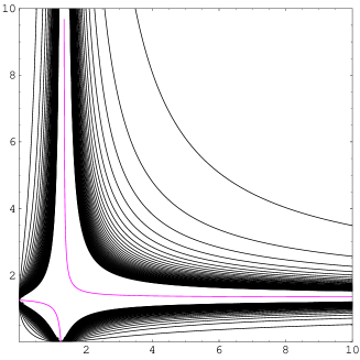
FIG. 2.: A contour plot of the transmission in the X${}_{\ell}-$X_r plane, for the same parameters as in Fig. 1. The resonance lines are the colored curves in the figure.

Next we calculate the charge, Q, pumped through the quantum dot during a single period of the modulation. Here we employ an expression which gives Q in terms of matrix elements of the temporal derivative of the scattering potential, $\dot{V}$, between the instantaneous scattering states. [22, 23] At zero temperature the charge per period reads

$${\rm Q}=\frac{e}{4\pi}\oint dt\Bigl{[}\langle\chi^{t}_{r}|\dot{V}|\chi^{t}_{r}\rangle-\langle\chi^{t}_{\ell}|\dot{V}|\chi^{t}_{\ell}\rangle\Bigr{]}.$$ (22)

This expression can be shown to reproduce the Brouwer [21] formula. [22]

In our model, the temporal derivative of the potential is

$$\dot{V}(n,n^{\prime}) = -\dot{J}_{\ell}\Bigl{(}\delta_{n,1}\delta_{n^{\prime},0}+\delta_{n^{\prime},1}\delta_{n,0}\Bigr{)}$$ (23)

$$- \dot{J}_{r}\Bigl{(}\delta_{n,N}\delta_{n^{\prime},N+1}+\delta_{n^{\prime},N}\delta_{n,N+1}\Bigr{)},$$ (24)

and hence the charge pumped from left to right is

$${\rm Q} = -\Re\Bigl{\{}\frac{e}{2\pi}\oint dt\Bigl{(}\dot{J}_{\ell}\Bigl{[}\chi^{t\ast}_{r}(0)\chi^{t}_{r}(a)-\chi^{t\ast}_{\ell}(0)\chi^{t}_{\ell}(a)\Bigr{]}$$ (25)

$$+ \dot{J}_{r}\Bigl{[}\chi^{t\ast}_{r}(Na)\chi^{t}_{r}((N+1)a)$$ (26)

$$- \chi^{t\ast}_{\ell}(Na)\chi^{t}_{\ell}((N+1)a)\Bigr{]}\Bigr{)}\Bigr{\}}.$$ (27)

This expression requires the knowledge of the scattering solutions on the two ends of the quantum dot. These are given by using Eqs. (5) and (7),

$$\chi^{t}_{\ell}(a) = \frac{1}{J_{\ell}}A_{0,\ell}\Bigl{(}e^{ika}+r_{t}e^{-ika}\Bigr{)},$$ (28)

$$\chi^{t}_{\ell}(Na) = \frac{1}{J_{r}}A_{0,\ell}t_{t}e^{ikNa},$$ (29)

$$\chi^{t}_{r}(a) = \frac{1}{J_{\ell}}A_{0,r}t_{t}e^{-ika},$$ (30)

$$\chi^{t}_{r}(Na) = \frac{1}{J_{r}}A_{0,r}\Bigl{(}e^{-ikNa}+r^{\prime}_{t}e^{ikNa}\Bigr{)},$$ (31)

together with the results in Eq. (13). It then follows that the pumped charge, Q, is given by

$${\rm Q} = \frac{e}{2\pi}\oint dt\frac{J_{\rm D}\sin Nqa\sin ka}{|D_{k}|^{2}}$$ (33)

$$\times\Bigl{[}\Bigl{(}{\rm X}_{\ell}\dot{\rm X}_{r}-{\rm X}_{r}\dot{\rm X}_{\ell}\Bigr{)}J_{\rm D}E_{k}\sin Nqa$$

$$+ \Bigl{(}{\rm X}^{2}_{\ell}\dot{\rm X}_{r}-{\rm X}_{r}^{2}\dot{\rm X}_{\ell}\Bigr{)}\sin(N-1)qa$$ (34)

$$+ \Bigl{(}\dot{\rm X}_{r}-\dot{\rm X}_{\ell}\Bigr{)}J_{\rm D}^{2}\sin(N+1)qa\Bigr{]}.$$ (35)

The temporal integration in this expression, with the time dependence as given by Eq. (2), is now done analytically, separating the four poles of the denominator in $\cos\omega t$. The results, for a selected set of parameters, are shown in Fig. 1.

We now relate the values of Q, for representative values of the pumping amplitude P, to the pumping contour, which is the closed curve the system traverses during a single cycle in the X${}_{\ell}-$X_r plane. Those curves are portrayed in Figs. 3 (P=1), 4 (P=3), 5 (P=5), and 6 (P=10). In each of the these figures, the left plate shows the contours of equal transmission (in black), the resonance lines (in red) and that section of the pumping contour which lies near the transmission maxima (in blue). The right plate exhibits the full pumping contour. (The numbers on the axes in the right plate indicate the scale of the pumping contour.) We begin with the situation at P=1. At this value, as can be seen from Fig. 1, the charge pumped is vanishingly small. At this value, the pumping contour indeed encloses only a small portion of the resonance line, far away from the transmission maxima (see Fig. 3).

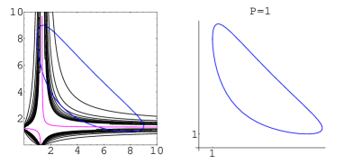
FIG. 3.: The pumping curve in the X${}_{\ell}-$X_r plane, for P=1. The other parameters are the same as in Fig. 1. The right plate shows the full pumping contour; The left one depicts the contours of equal transmission (in black), the resonance lines (in red), and the pumping contour (in blue).

Next, we consider the case P=3, for which the pumped charge is close to $-1$ (in units of $e$). Examining Fig. 4, it is seen that in this case the pumping contour encloses only the upper resonance line, including the transmission peak there. For this value of P, the pumping contour begins to fold on itself (since X_ℓ and X_r are definitely positive), forming a Lissajous curve in that parameter plane. This tendency is of course enhanced as the pumping amplitude P increases. The charge remains close to $-1$ as long as the pumping contour remains between the two branches of the resonance line, as in Fig. 4.

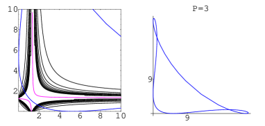
FIG. 4.: The same as Fig. 3, but for P=3. The other parameters are the same as in Fig. 1.

Moving to the case P=5 (Fig. 5), at which the pumped charge is small and positive (see Fig. 1), we find that now the pumping contour encircles both transmission peaks on the resonance lines; The separate contributions of the two resonances to the temporal integration in Eq. (35) almost cancel one another, leading to a rather tiny value for the charge.

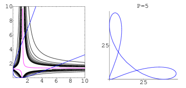
FIG. 5.: The same as Fig. 3, but for P=5. The other parameters are the same as in Fig. 1.

Finally, we consider the case P=10. The left plate in Fig. 6 is similar to the left one in Fig. 4, and indeed, the absolute value of Q is close to the one in both cases. However, the sense in which the pumping contour encircles the resonance is reversed in the two cases, as can be gathered by examining the right plates in Figs. 4 and 6. Hence, the pumped charge changes sign.

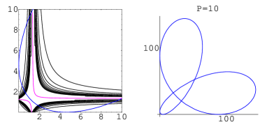
FIG. 6.: The same as Fig. 3, but for P=10. The other parameters are the same as in Fig. 1.

We now examine the pumping when the phase shift $\phi$ of the modulation [see Eq. (2)] is changed. Instead of taking $\phi=0.4\pi$, which was used to plot the previous figures, we now choose $\phi=0.05\pi$, keeping all other parameters as before. Although one might have thought that this smaller value will reduce the magnitude of the pumped charge, we now find that $|{\rm Q}|$ attains the value of $2$, see Fig. 7.

FIG. 7.: The pumped charge, Q, in units of $e$, as function of the modulating amplitude, P. The parameters are the same as in Fig. 1, except that $\phi=0.05\pi$.

The next five figures portray the pumping contours relation to the resonance lines for representative values of the amplitude P, for the parameters of Fig. 7. In Fig. 8 we have P=1. Then the pumping contour encloses just a small part of the upper resonance line, and also touches the peak on the lower resonance line. Indeed, Q has an intermediate value near $-0.5$, decreasing to zero as P moves away from 1 (see Fig. 7).

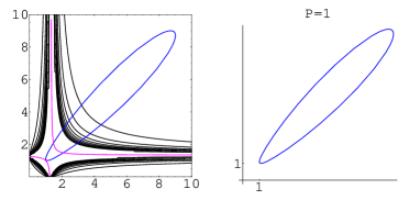
FIG. 8.: The pumping curve in the X${}_{\ell}-$X_r plane, for P=1. The other parameters are the same as in Fig. 7. The right plate shows the full pumping curve; The left one depicts the contours of equal transmission (in black), the resonance lines (in red), and the pumping contour (in blue).

Increasing the amplitude to the value P=3 reveals that the pumping contour encloses both peaks on the resonance lines, and therefore their separate contributions almost cancel one another, leading to a tiny value of Q. Also, the pumping curve begins to fold on itself, giving rise to the small “bubble” close to the origin (see Fig. 9). Following the increase of that bubble as P in enhanced leads to the situation in which the bubble encloses the lower resonance, and then the charge attains the value 1 (see Fig. 7). As the bubble increases further, capturing the two resonance lines, as shown in Fig. 10, Q again becomes very small.

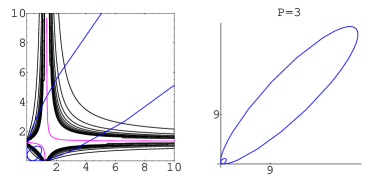
FIG. 9.: The same as Fig. 8, but for P=3. The other parameters are the same as in Fig. 7.

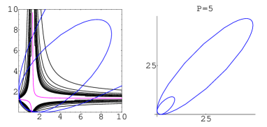
FIG. 10.: The same as Fig. 8, but for P=5. The other parameters are the same as in Fig. 7.

As P grows on, we reach the interesting situation, depicted in Fig. 11 for P=8, in which the bubble encircles twice the upper resonance line, leading to a pumped charge very close to $|2e|$.

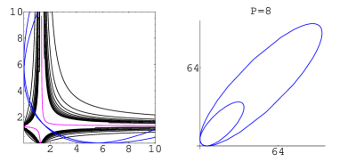
FIG. 11.: The same as Fig. 8, but for P=8. The other parameters are the same as in Fig. 7.

Finally, Fig. 12 shows the pumping contour for P=12. The contour is seen to shift away from the resonance peaks, yielding a vanishingly small value for Q.

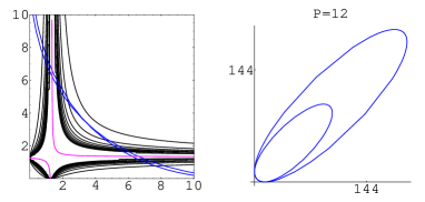
FIG. 12.: The same as Fig. 8, but for P=12. The other parameters are the same as in Fig. 7.

III Conclusions

We have calculated the charge passing through a small quantum dot whose point contact conductances are modulated periodically in time. The calculation is carried out for non-interacting electrons, under the assumption that the modulation frequency is much smaller than the electronic relaxation rates. We have found the conditions for obtaining integral values for the pumped charge: The contour traversed by the system in the parameter plane spanned by the pumping parameters (in our case, the point contact conductances) should encircle a significant portion of a resonance line (along which the transmission of the quantum contact is optimal) in that plane. The magnitude and the sign of the pumped charge are determined by that portion, and by the direction along which the resonance line is encompassed.

The reason for this observation can be traced back to the expression for the pumped charge, Eqs. (22) and (35). The contribution to the temporal integration comes mainly from the poles in the denominator in Eq. (35). These same poles are also responsible for the resonant states of the nanostructure, that is, for the maxima in the transmission coefficient. [17, 22, 23] In this way, we have obtained a topological description for the phenomenon of adiabatic charge pumping. One can now imagine more complex scenarios: including higher harmonics of $\omega$ in the time dependence of the point contact conductances can create more complex Lissajoux contours, which might encircle portions of the resonance lines more times, yielding higher quantized values of the pumped charge.

Finally, it should be mentioned that the results presented above are obtained at zero temperature. At finite temperatures, the expression for Q should be integrated over the the electron energy $E_{k}$, with the Fermi function derivative $-\partial f/\partial E_{k}$.[22, 23] Hence, upon the increase of the temperature, the pumped charge would be smeared and suppressed. It would be very interesting to check the above predictions in more complicated models (for example, when there are several levels on each of the sites forming the quantum dot), allowing for a richer structure of the transmission in the parameter space, and, of course, in real systems.

- [1] D. J. Thouless, Phys. Rev. B 27, 6083 (1983).
- [2] Q. Niu and D. J. Thouless, J. Phys. A 17, 2453 (1984).
- [3] Q. Niu, Phys. Rev. Lett. 64, 1812 (1990).
- [4] F. Hekking and Yu. V. Nazarov, Phys. Rev. B 44, 9110 (1991).
- [5] B. L. Altshuler and L. I. Glazman, Science 283, 1864 (1999).
- [6] L. J. Geerligs, V. F. Anderegg, P. A. M. Holweg, J. E. Mooij, H. Pothier, D. Esteve, C. Urbina, and M. H. Devoret, Phys. Rev. Lett. 64, 2691 (1990).
- [7] L. P. Kouwenhoven, A. T. Johnson, N. C. van der Vaart, A. van der Enden, C. J. P. M. Harmans, and C. T. Foxon, Z. Phys. B85, 381 (1991).
- [8] H. Pothier, P. Lafarge, U. Urbina, D. Esteve and M. H. Devoret, Europhys. Lett. 17, 249 (1992).
- [9] M. Switkes, C. M. Marcus, K. Campman and A. C. Gossard, Science 283, 1905 (1999).
- [10] J. M. Shilton, V. I. Talyanskii, M. Pepper, D. A. Ritchie, J. E. F. Frost, C. J. Ford, C. G. Smith and G. A. C. Jones, J. Phys.: Condens. Matter 8, L531 (1996).
- [11] V. I. Talyanskii, J. M. Shilton, M. Pepper, C. G. Smith, C. J. Ford, E. H. Linfield, D. A. Ritchie, and G. A. C. Jones, Phys. Rev. B 56, 15180 (1997).
- [12] V. I. Talyanskii, D. S. Novikov, B. D. Simons, and L. S. Levitov, Phys. Rev. Lett. 87, 276802 (2001).
- [13] I. L. Aleiner and A. V. Andreev, Phys. Rev. Lett. 81, 1286 (1998).
- [14] T. A. Shutenko, I. L. Aleiner and B. L. Altshuler, Phys. Rev. B 61, 10366 (2000).
- [15] J. E. Avron, A. Elgart, G. M. Graf, and L. Sadun, Phys. Rev. Lett. 87, 236601 (2001).
- [16] Y. Makhlin and A. D. Mirlin, Phys. Rev. Lett. 87, 276803 (2001).
- [17] Y. Levinson, O. Entin-Wohlman, and P. Wölfle, Physica A 302, 335 (2001).
- [18] Y. Wei, J. Wang, and H. Gou, Phys. Rev. B 62, 9947 (2000).
- [19] Y. Wei, J. Wang, H. Guo, and C. Roland, Phys. Rev. B 64, 115321 (2001).
- [20] T. K. Ng and P. A. Lee, Phys. Rev. Lett. 61, 1768 (1988).
- [21] P. W. Brouwer, Phys. Rev. B 58, R10135 (1998).
- [22] O. Entin-Wohlman, A. Aharony, and Y. Levinson, cond-mat/0201073.
- [23] A. Aharony and O. Entin-Wohlman, cond-mat/0111053.