Permutation zones and the fermion sign problem

Abstract

We present a new approach to the problem of alternating signs for fermionic many body Monte Carlo simulations.  We demonstrate that the exchange of identical fermions is typically short-ranged even when the underlying physics is dominated by long distance correlations.  We show that the exchange process has a maximum characteristic range of $\sqrt{2(1-f)\beta h}$ lattice sites, where $\beta$ is the inverse temperature, $h$ is the hopping parameter, and $f$ is the filling fraction.  We introduce the notion of permutation zones, special regions of the lattice where identical fermions may interchange and outside of which they may not.   Using successively larger permutation zones, one can extrapolate to obtain thermodynamic observables in regimes where direct simulation is impossible.

I Introduction

One of the most important challenges for quantum field theory and many body simulations is the study of light fermion dynamics.  Today most fermion algorithms used in lattice field theory are based on pseudofermion methods, which calculate the contribution of fermions indirectly by means of an effective non-local bosonic action. The most popular approach, Hybrid Monte Carlo, deals directly with non-local actions [1].  Molecular dynamics is used to propose new configurations and a Metropolis criterion is used to accept or reject updates.  Although the advantages of pseudofermion methods are substantial, there are still important motivations for doing simulations with explicit fermions.  The primary concern is the question of what fermions actually do in lattice simulations.  In lattice gauge theory, for example, one might be interested in seeing the effects of confinement on quark-antiquark pair separation or the relation between chiral symmetry breaking and light quark mobility.  These questions are most easily addressed in a local field framework which keeps the fermionic degrees of freedom explicit.

In order to do get anywhere with explicit fermion simulations one must of course address the fermion sign problem. In this paper we introduce a new approach to the sign problem which has applications to quantum simulations at finite temperature.  Unlike the fixed-node approach [2, 3, 4], our method makes no assumption about the nodal structure of the eigenfunctions.  It also is not a resummation technique, the underlying principle powering the meron-cluster algorithm [5] and diagonalization/Monte Carlo methods [6, 7].  The approach we introduce here is based on the observation that in most finite temperature simulations fermion permutations are short ranged.  This holds true even for systems with massless modes and long distance correlations, as we demonstrate with two examples.  In this paper we focus on the application of the zone method to simulations with explicit fermions.  These methods have recently been applied to study chiral symmetry breaking in massless quantum electrodynamics in $2+1$ dimensions [8].  The extension to pseudofermion methods and, in particular, applications to Euclidean lattice gauge theory will be discussed in a future publication.

II Worldlines

We begin with a brief review of the worldline formalism [9].  We introduce the basic ideas in one spatial dimension before moving on to higher dimensions.  Let us consider a system with one species of fermion on a periodic chain with $L$ sites, where $L$ is even.  Aside from an additive constant, the general Hamiltonian can be written as

$$H=-h\sum_{i}\left[a_{i+1}^{\dagger}a_{i}+a_{i}^{\dagger}a_{i+1}\right]+\sum_{i}c_{i}a_{i}^{\dagger}a_{i}.$$ (1)

Following [9] we break the Hamiltonian into two parts, $H_{\text{e}}$ and $H_{\text{o}}$,

$$H_{\text{e/o}}=\sum_{i\text{ even/odd}}\left[\begin{array}[]{c}-ha_{i+1}^{\dagger}a_{i}-ha_{i}^{\dagger}a_{i+1}\\ +{\textstyle{c_{i}\over 2}}a_{i}^{\dagger}a_{i}+{\textstyle{c_{i+1}\over 2}}a_{i+1}^{\dagger}a_{i+1}\end{array}\right].$$ (2)

We note that $H=H_{\text{e}}+H_{\text{o}}$.

We are interested in calculating thermal averages,

$$\left\langle O\right\rangle=\frac{Tr\left[O(a^{\dagger},a)\exp(-\beta H)\right]}{Tr\left[\exp(-\beta H)\right]},$$ (3)

where $\beta=(k_{B}T)^{-1}$.  For large $N$, we can write

$$\exp(-\beta H)=\left[\exp\left[-{\textstyle{\beta\over N}}(H_{\text{e}}+H_{\text{o}})\right]\right]^{N}\approx(S_{\text{o}}S_{\text{e}})^{N},$$ (4)

where

$$S_{\text{e/o}}=\exp(-{\textstyle{\beta\over N}}H_{\text{e/o}}).$$ (5)

Inserting a complete set of states at each step, we can write $Tr\left[\exp(-\beta H)\right]$ as

$$\sum_{z_{0},...,z_{2N-1}}\left\langle z_{0}\right|S_{\text{o}}\left|z_{2N-1}\right\rangle...\left\langle z_{1}\right|S_{\text{e}}\left|z_{0}\right\rangle.$$ (6)

In Fig. 1 a typical set of states $\left|z_{0}\right\rangle,...,\left|z_{2N-1}\right\rangle$ are shown which contribute to the sum in (6).  We call such a contribution a worldline configuration.  The shaded plaquettes represent locations where $S_{\text{e}}$ or $S_{\text{o}}$ acts on the corresponding local fermionic state.  The classical trajectory of each of the fermions can be traced from Euclidean time $t=0$ to time $t=\beta$.  In the case when two identical fermions enter the same shaded plaquette, we adopt the convention that the worldlines run parallel and do not cross.  With this convention the fermion sign associated with Fermi statistics is easy to compute.  The worldlines from $t=0$ to $t=\beta$ define a permutation of identical fermions.  Even permutations carry a fermion sign of $+1$ while odd permutations carry sign $-1$.  The generalization to higher dimensions is straightforward.  In two dimensions, for example, $\exp(-\beta H)$ takes the form

$$\left.\begin{array}[]{c}\left[\exp\left[-{\textstyle{\beta\over N}}(H_{\text{e}}^{x}+H_{\text{o}}^{x}+H_{\text{e}}^{y}+H_{\text{o}}^{y})\right]\right]^{N}\\ \qquad\qquad\qquad\approx(S_{\text{o}}^{y}S_{\text{e}}^{y}S_{\text{o}}^{x}S_{\text{e}}^{x})^{N}.\end{array}\right.$$ (7)

The sum over all worldline configurations can be calculated with the help of the loop algorithm [10].  At each occupied/unoccupied site, we place an upward/downward pointing arrow as shown in Fig. 2.  Due to fermion number conservation, the number of arrows pointing into a plaquette equals the number of arrows pointing out of the plaquette.  New Monte Carlo updates of the worldlines are produced by flipping the arrows which form closed loops.

III Wandering length

In one spatial dimension, the Pauli exclusion principle inhibits fermion permutations except in cases where the fermions wrap around the lattice boundary.  For the remainder of our discussion, therefore, we consider systems with two or more dimensions.  The first question we address is how far fermion worldlines can wander from start time $t=0$ to end time $t=\beta$.  We can put an upper bound on this wandering distance by considering the special case with no on-site potential and only nearest neighbor hopping.

Let us consider motion in the $x$-direction.  For each factor of $S_{\text{o}}^{x}S_{\text{e}}^{x}$ in (7) a given fermion may remain at the same $x$ value, move one lattice space to the left, or move one lattice space to the right.  If $h$ is the hopping parameter, then for large $N$ the relative weights for these possibilities are approximately $1$ for remaining at the same $x$ value, $\beta hN^{-1}$ for one move to the left, and $\beta hN^{-1}$ for one move to the right.  In (7) we see that there are $N$ factors of $S_{\text{o}}^{x}S_{\text{e}}^{x}$.  Therefore for a typical worldline configuration at low filling fraction, $f,$ we expect $\sim\beta h$ hops to the left and $\sim\beta h$ hops to the right.  For non-negligible $f$ some of the hops are forbidden by the exclusion principle.  Assuming random filling we expect $\sim(1-f)\beta h$ hops to the left and $\sim(1-f)\beta h$ hops to the right.

The net displacement is equivalent to a random walk with $2(1-f)\beta h$ steps.  The expected wandering length, $\Delta,$ is therefore given by

$$\Delta=\sqrt{2(1-f)\beta h}.$$ (8)

This result is somewhat surprising in that for typical simulation parameters (i.e., $\beta$ not too large), we find $\Delta$ is no larger than a few lattice units.  There is no contradiction between the existence of long distance correlations and the constraint of short distance wandering lengths.  Long range signals are propagated by the net effect of many short range displacements.  A simple analogy can be made with electrical conduction in a wire or sound propagation in a gas, which results from many short range displacements of individual electrons or gas molecules.

In cases with on-site potentials, fermion hopping is dampened by differences in potential energy.  Hence the estimate (8) serves as an upper bound for the general case.  We have checked the upper bound numerically using simulation data generated by several different lattice Hamiltonians with and without on-site potentials.

IV Permutation Zone Method

Let $W$ be the logarithm of the partition function,

$$W=\log\left\{Tr\left[\exp(-\beta H)\right]\right\}.$$ (9)

Let us partition the spatial lattice, $\Gamma$, into zones $Z_{1},Z_{2},...,Z_{k}$ such that the spatial dimensions of each zone are much greater than $\Delta$.  For notational convenience we define $Z_{0}=\emptyset$.  For any $R\subset\Gamma$, let $W_{R}$ be the logarithm of a restricted partition function that includes only worldline configurations where any worldline starting outside of $R$ at $t=0$ returns to the same point at $t=\beta$.  In other words there are no permutations for worldlines starting outside of $R$. We note that $W_{\Gamma}=W,$ and $W_{\emptyset}$ is the logarithm of the restricted partition function with no worldline permutations at all.  Since the zones are much larger than the length scale $\Delta$, the worldline permutations in one zone has little or no effect on the worldline permutations in another zones.  Therefore

$$W_{Z_{0}\cup...\cup Z_{j}}-W_{Z_{0}\cup...\cup Z_{j-1}}\approx W_{Z_{j}}-W_{\emptyset}.$$ (10)

Using a telescoping series, we obtain

$$W_{\Gamma}-W_{\emptyset} = \sum_{j=1,...,k}(W_{Z_{0}\cup...\cup Z_{j}}-W_{Z_{0}\cup...\cup Z_{j-1}})$$ (11)

$$\approx \sum_{j=1,...,k}(W_{Z_{j}}-W_{\emptyset}).$$ (12)

For translationally invariant systems tiled with congruent zones we find

$$W=W_{\Gamma}\approx W_{\emptyset}+{\textstyle{\left|\Gamma\right|\over\left|Z_{1}\right|}}(W_{Z_{1}}-W_{\emptyset}),$$ (13)

where $\left|\Gamma\right|/\left|Z_{1}\right|=k$, the number of zones.  For general zone shapes one can imagine partitioning the zones themselves into smaller congruent tiles.  Therefore the result (13) should hold for large arbitrarily shaped zones.  For this case we take $\left|\Gamma\right|$ to be the number of nearest neighbor bonds in the entire lattice and $\left|Z_{1}\right|$ to be the number of nearest neighbor bonds in the zone.  We will refer to $\left|Z_{1}\right|$ as the zone size of $Z_{1}$.  This is just one choice for zone extrapolation.  A more precise and complicated scheme could be devised which takes into account the circumscribed volume, number of included lattice points, and other geometric quantities.

V Free fermions

As an example of the zone method, we compute the average energy $\left\langle E\right\rangle h^{-1}$ for a free fermion Hamiltonian with only hopping interactions on an $8\times 8$ lattice.  We consider values $\beta h=1.0$, $1.5$, and $2.0$.  The corresponding values for $\Delta$ are $1.0$, $1.2$, and $1.4$ respectively.  The Monte Carlo updates are performed using a single loop flip version of the loop algorithm [10].

In Fig. 3 we show data for rectangular zones with side dimensions $0\times 0$, $1\times 1$, $2\times 1$, $2\times 2$, $3\times 2$, $3\times 3$, …, $6\times 6$.  We also show a least-squares fit (not including the smallest zones $0\times 0$ and $1\times 1$) assuming linear dependence on zone size as predicted in (13).  We find agreement at the $1\%$ level or better when compared with the exact answers shown on the far right, which were computed using momentum-space decomposition.

While the physics of the free hopping Hamiltonian is trivial, the computational problems are in fact maximally difficult.  The severity of the sign problem can be measured in terms of the average sign, $<$Sign$>$, for contributions to the partition function.  For $\beta h=1.0$, $<$Sign$>\sim 0.005;$ for $\beta h=1.5$, $<$Sign$>$ $\sim 10^{-6};$ and for $\beta h=2.0$, $<$Sign$>$$\sim 10^{-9}$.  Direct calculation using position-space Monte Carlo is impossible by several orders of magnitude for $\beta h\geq 1.5$.

VI Fermionic 2D Ising Model

While the free fermion example shows the linear dependence on zone size, we now study an example which better demonstrates the utility of the zone method.  We will consider the Hamiltonian,

$$H = J\sum_{i,j}\left[s_{i,j}s_{i+1,j}+s_{i,j}s_{i,j+1}\right]$$ (15)

$$-h\sum_{i,j}\left[a_{i+1,j}^{\dagger}a_{i,j}+a_{i,j}^{\dagger}a_{i+1,j}+a_{i,j+1}^{\dagger}a_{i,j}+a_{i,j}^{\dagger}a_{i,j+1}\right],$$

where

$$s_{i,j}=2a_{i,j}^{\dagger}a_{i,j}-1=2n_{i,j}-1.$$ (16)

We will refer to this model as the fermionic 2D Ising model.  When $h=0$, our model reduces to the antiferromagnetic 2D Ising model for $J>0$ and the regular 2D Ising model for $J<0$, with $2n_{i,j}-1$ playing the role of Ising spin.  We also note that the model for $h>0$ is equivalent to the $h<0$ model.  On an even lattice, we can reverse the sign of $h$ by multiplying $-1$ to all creation and annihilation operators on sites where $i+j$ is odd.  Unlike other quantum generalizations such as the transverse field Ising model (see for example [11]), we have reinterpreted the Ising spin as an occupation number and introduced nearest neighbor hopping of Fermi-Dirac particles.

To our knowledge the fermionic Ising model has not previously been discussed in the literature.  Therefore let us briefly discuss our interest in the model.  The model is motivated by our studies of time-dependent background field fluctuations in Hamiltonian lattice gauge theories.  In lattice gauge theory we encounter time-dependent Hamiltonians which in the Kogut-Susskind staggered formalism [12] have the form

$$H(t)=\sum_{i,j}\left[H_{1,i,j}(t)+H_{2,i,j}(t)\right]+...,$$ (17)

where

$$H_{1,i,j}(t) = \sum_{m,n}\left[-(h_{1,i,j}^{m,n}(t))^{\ast}a_{i+1,j}^{n\dagger}a_{i,j}^{m}-h_{1,i,j}^{m,n}(t)a_{i,j}^{m\dagger}a_{i+1,j}^{n}\right],$$ (18)

$$H_{2,i,j}(t) = \sum_{m,n}\left[-(h_{2,i,j}^{m,n}(t))^{\ast}a_{i,j+1}^{n\dagger}a_{i,j}^{m}-h_{2,i,j}^{m,n}(t)a_{i,j}^{m\dagger}a_{i,j+1}^{n}\right].$$ (19)

The indices $m$ and $n$ are gauge group indices, and $h_{1,i,j}^{m,n}(t)$ and $h_{2,i,j}^{m,n}(t)$ are background gauge fields.  We will consider a simplified version of this system, where

$$H_{1,i,j}(t) = -h_{1,i,j}(t)\left(a_{i+1,j}^{\dagger}a_{i,j}+a_{i,j}^{\dagger}a_{i+1,j}\right),$$ (20)

$$H_{2,i,j}(t) = -h_{2,i,j}(t)\left(a_{i,j+1}^{\dagger}a_{i,j}+a_{i,j}^{\dagger}a_{i,j+1}\right),$$ (21)

and $h_{1,i,j}(t)$ and $h_{2,i,j}(t)$ are real valued functions.  Let us consider what happens when $h_{1,i,j}(t)$ and $h_{2,i,j}(t)$ are subject to Gaussian fluctuations.  Let us define the Gaussian-integrated exponentials of the Hamiltonian,

$$A_{1,i,j} = \int dh_{1,i,j}(t)\;\exp\left[-dt\cdot H_{1,i,j}(t)\right]\exp\left[-dt\cdot{\textstyle{1\over 8J}}(h_{1,i,j}(t)-h)^{2}\right],$$ (22)

$$A_{2,i,j} = \int dh_{2,i,j}(t)\;\exp\left[-dt\cdot H_{2,i,j}(t)\right]\exp\left[-dt\cdot{\textstyle{1\over 8J}}(h_{2,i,j}(t)-h)^{2}\right].$$ (23)

We find

$$A_{1,i,j} \varpropto \exp\left[dt\cdot h\left(a_{i+1,j}^{\dagger}a_{i,j}+a_{i,j}^{\dagger}a_{i+1,j}\right)+dt\cdot 2J\left(a_{i+1,j}^{\dagger}a_{i,j}+a_{i,j}^{\dagger}a_{i+1,j}\right)^{2}\right],$$ (24)

$$A_{2,i,j} \varpropto \exp\left[dt\cdot h\left(a_{i,j+1}^{\dagger}a_{i,j}+a_{i,j}^{\dagger}a_{i,j+1}\right)+dt\cdot 2J\left(a_{i,j+1}^{\dagger}a_{i,j}+a_{i,j}^{\dagger}a_{i,j+1}\right)^{2}\right].$$ (25)

We note that

$$\left(a_{i+1,j}^{\dagger}a_{i,j}+a_{i,j}^{\dagger}a_{i+1,j}\right)^{2} = {\textstyle{1\over 2}}\left(-s_{i+1,j}s_{i,j}+1\right),$$ (26)

$$\left(a_{i,j+1}^{\dagger}a_{i,j}+a_{i,j}^{\dagger}a_{i,j+1}\right)^{2} = {\textstyle{1\over 2}}\left(-s_{i,j}s_{i,j+1}+1\right),$$ (27)

and so the effect of such fluctuations is exactly modelled by an effective Hamiltonian of the form (15) for $J>0$.  In the staggered formalism, fermion spin states are staggered at odd and even lattice sites, and the onset of antiferromagnetic order corresponds with the spontaneous breaking of chiral symmetry.

The sign problem makes it difficult to study the fermionic Ising model at large volumes.  There is no existing method that can handle this model with explicit fermionic degrees of freedom.  For example near the transition temperature for $h/J=2.00$ on a $20\times 20$ lattice we find $<$Sign$>$$\sim 10^{-4}$.  Given the significant computational difficulties we would like to see if the zone method could be effective for explicit fermion simulations near the critical temperature.  One might expect the zone method to be useful since all of the physics of the $h=0$ Ising model is already contained in $W_{\emptyset}$, the logarithm of the restricted partition function with no worldline permutations.  For $h\neq 0$ the contributions due to fermion permutations can be included in a controlled manner by considering successively larger permutation zones.

Let us define the spontaneous staggered magnetization $\left\langle S\right\rangle$ as

$$\left\langle S\right\rangle=(-1)^{i+j}\left\langle s_{i,j}\right\rangle=(-1)^{i+j}\left\langle 2n_{i,j}-1\right\rangle.$$ (28)

We will compute $\left\langle S\right\rangle$ for various temperatures and values $h/J$ while adding a small external bias

$\displaystyle H\rightarrow H-m\sum_{i,j}(-1)^{i+j}s_{i,j}.$

We compute $\left\langle S\right\rangle$ by linearly extrapolating results for different permutation zone sizes.  For $h/J\leq 1,$ the sign problem is significant but still manageable on a $20\times 20$ lattice near the critical point.  For $h/J>1$, full simulations on a $20\times 20$ lattice are not practical due to the sign.  For $h/J=1.50$ we use permutation zones as large as $10\times 10$, and for $h/J=2.00$ we extrapolate using zones up to $6\times 6$.  In Fig. 4 we show the zone extrapolation for the staggered magnetization $\left\langle S\right\rangle$ at $h/J=1.50$, $T/J=2.00$, and $m/J=0.0256$ on a $20\times 20$ lattice.  In Fig. 5 we plot the zone-extrapolated results as a function of $T/J$ near the critical temperature for $h/J=1.50$, $m/J=0.0256$.  Since the hopping interaction increases the disorder of the system, we expect the critical temperature to decrease as $h$ increases.  Noting that the $h=0$ Ising model has a critical temperature

$$T_{c}^{\text{Ising}}/J={\textstyle{2\over\ln(1+\sqrt{2})}}\approx 2.269,$$ (29)

we see that the data in Fig. 5 does in fact show a decrease in the critical temperature.  We also find a critical exponent of $\beta=0.10(2)$, which is consistent with that of the Ising model, $\beta_{\text{Ising}}=0.125.$

In Fig. 6 we show the deviation of the critical temperature from $T_{c}^{\text{Ising}}$.  In our plot we have included errors due to finite size effects, which we found by recalculating results using $10\times 10$ and $16\times 16$ lattice sizes and several different values for $m/J$.  We note that the deviation of the critical temperature appears to be quadratic in $h/J,$ with possibly a small negative cubic contribution.  It would be interesting to carry these simulations further to see how the curve behaves for larger values of $h/J$.  About 2000 CPU hours on an IBM SP3 were used to collect the data for this study.

VII Summary

We have presented a promising new approach to fermionic simulations at finite temperatures.  We have demonstrated that the exchange of identical fermions is short-ranged and has a maximum range of $\sqrt{2(1-f)\beta h}$ lattice sites, where $\beta$ is the inverse temperature, $h$ is the hopping parameter, and $f$ is the filling fraction.  We have introduced the notion of permutation zones, special regions of the lattice where identical fermions may interchange and outside of which they may not.   Using successively larger zones, one can extrapolate to obtain thermodynamic observables.  We have demonstrated the method using two different examples:  the average energy for a 2D free fermion and the spontaneous staggered spin magnetization for the 2D fermionic Ising model.

The methods presented here are relatively easy to implement.  Correlation functions can be calculated using worm algorithms [13], which are generalizations of the loop algorithm.  Although the full applicability of the zone method still needs to be determined, the method and its future generalizations may have some impact on several problems in strongly correlated solid-state systems and lattice gauge theory.  In this paper we have focused on simulations with explicit fermion degrees of freedom.  The extension of the zone method to pseudofermion algorithms is currently being studied and will presented in a future publication.

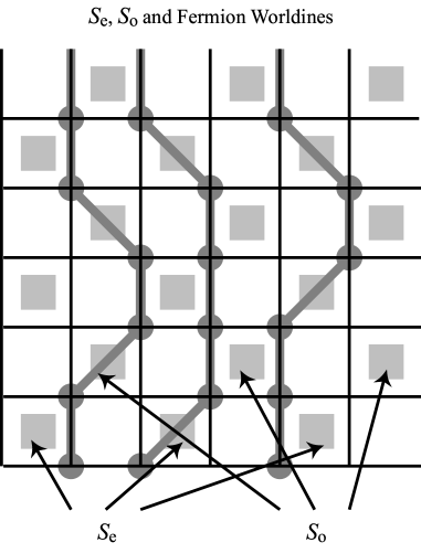
FIG. 1.: Typical worldline configuration for the one-dimensional system.

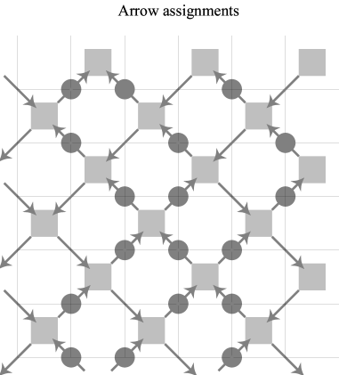
FIG. 2.: Upward/downward arrows are drawn at each occupied/unoccupied site. For each plaquette the number of inward-pointing arrows equals the number of outward-pointing arrows.

FIG. 3.: Average energy at $\beta h=1.0,1.5,2.0$ for free fermions on an $8\times 8$ lattice.

FIG. 4.: Zone extrapolation for the staggered magnetization $\left\langle S\right\rangle$ for the 2D fermionic Ising model at $h/J=1.50,T/J=2.00,m/J=0.0256.$

FIG. 5.: Staggered magnetization $\left\langle S\right\rangle$ for the 2D fermionic Ising model near the critical point for $h/J=1.50,m/J=0.0256$.

FIG. 6.: Change in the critical temperature of the 2D fermionic Ising model as a function of $h/J$.

- [1] S. Duane, A. Kennedy, B. Pendleton, D. Roweth, Phys. Lett. B195 216 (1987).
- [2] J. B. Anderson, J. Chem. Phys. 63 1499 (1975); J. Chem. Phys. 65 4121 (1976).
- [3] P. J. Reynolds, D. M. Ceperley, B. J. Alder, and W. A. Lester, Jr., J. Chem Phys. 77 5593 (1982).
- [4] J. W. Moskowitz, K. E. Schmidt, M. A. Lee, and M. H. Kalos, J. Chem. Phys. 77 349 (1982).
- [5] S. Chandrasekharan, U.-J. Wiese, Phys. Rev. Lett. 83, 3116 (1999).
- [6] D. J. Lee, N. Salwen, D. D. Lee, Phys. Lett. B 503 223-235 (2001).
- [7] D. Lee, N. Salwen, M. Windoloski, Phys. Lett. B 502 329-337 (2001).
- [8] P. Maris, D. Lee, hep-lat/0209052, to appear in the proceedings of Lattice 2002.
- [9] J. Hirsch, D. Scalapino, R. Sugar, R. Blankenbecler, Phys. Rev. Lett. 47 1628 (1981); Phys. Rev. B 26 5033 (1982).
- [10] H. G. Evertz, to appear in Numerical Methods of Lattice Quantum Many-Body Problems, edited by D. J. Scalapino, Perseus, Berlin, 2001; H. G. Evertz, G. Lana, M. Marcu, Phys. Rev. Lett. 70, 875 (1993); H. G. Evertz, M. Marcu in Quantum Monte Carlo Methods in Condensed Matter Physics, p. 65, edited by M. Suzuki, World Scientific, 1994.
- [11] S. Sachdev, Quantum Phase Transitions, Cambridge University Press, Cambridge, 1999.
- [12] L. Susskind, Phys. Rev. D 16, 3031 (1977).
- [13] N. Prokof’ev, B. Svistunov, I. Tupitsyn, Sov. Phys. - JETP 87, 310 (1998).