Steady state properties of a mean field model of driven inelastic mixtures.

Abstract

We investigate a Maxwell model of inelastic granular mixture under the influence of a stochastic driving and obtain its steady state properties in the context of classical kinetic theory. The model is studied analytically by computing the moments up to the eighth order and approximating the distributions by means of a Sonine polynomial expansion method. The main findings concern the existence of two different granular temperatures, one for each species, and the characterization of the distribution functions, whose tails are in general more populated than those of an elastic system. These analytical results are tested against Monte Carlo numerical simulations of the model and are in general in good agreement. The simulations, however, reveal the presence of pronounced non-gaussian tails in the case of an infinite temperature bath, which are not well reproduced by the Sonine method.

I Introduction

Granular materials, a term coined to classify assemblies of macroscopic dissipative objects, are ubiquitous in nature and play a major role in many industrial and technological processes.

Interestingly, when a rarefied granular system is vibrated some of its properties are similar to those of molecular fluids, while others are unique and have no counterpart in ordinary fluids general . A spectacular manifestation of this difference can be observed in a driven mixture of granular particles: if one measures the average kinetic energy per particle, proportional to the so called granular temperature, one finds the surprising result that each species reaches a different value. Such a feature, observed in a recent experiment Menon , is in sharp contrast with the experience with other states of matter. At a more fundamental level such a behavior is in conflict with the Zeroth Law of thermodynamics. This principle states that when two systems globally isolated are brought into thermal contact they exchange energy until they reach a stationary state of mutual equilibrium, characterized by the same value of their temperatures. A corollary to such a principle is the statement that the thermal equilibrium between systems A and B, i.e. $T_{A}=T_{B}$, and between A and C ($T_{A}=T_{C}$) implies the thermal equilibrium between B and C Pippard .

On the contrary, when two granular system A and B subject to an external driving force exchange energy they may reach in general a mutual equilibrium, characterized by two constant but different granular temperatures $T_{A}$ and $T_{B}$. In addition even when A and C are in equilibrium at the same temperature $T_{C}$ and B and C also have the temperature $T_{C}$ one cannot conclude that A and B would be in mutual equilibrium at the same temperature. In other words, one of the most useful properties of the temperature, i.e. the independence from the thermal substance is lost when one deals with granular materials.

In the present paper we shall investigate the properties of a simple model of two component granular mixture. The motivation of our study relies in the fact that granular materials being mesoscopic objects are often constituted by assemblies of grains of different sizes and/or different physical and mechanical properties. The study of granular mixtures has attracted so far the attention both of theoreticians Dufty and of experimentalists Menon . In particular Garzó and Dufty have studied the evolution of a mixture of inelastic hard spheres in the absence of external driving forces, a process termed free cooling because associated with a decrease of the average kinetic energy of the system, i.e. of its granular temperature. During the cooling of a mixture, which can be homogeneous or not, according to the presence of spatial density and velocity gradients, each species may have different granular temperatures, although these may result asymptotically proportional, i.e. they might decrease at the same rate.

Menon and Feitosa instead studied several mixtures of vibrated inelastic grains and reported their failure to reach the same granular temperature.

In the present paper our interest will be concentrated on the statistically stationary state obtained by applying an energy feeding mechanism represented by a stochastic driving force.

The most widely used model of granular materials is, perhaps, the inelastic hard sphere model (IHS) IHS , which assumes the grains to be rigid and the collisions to be binary, instantaneous and momentum conserving. The dissipative nature of the collisions is accounted for by values less than $1$ of the so called restitution coefficient $r$. Even such an idealized model represents a hard problem to the theorist and one has to rely on numerical methods, namely Molecular Dynamics or Event Driven Simulation, or to resort to suitable truncation schemes of the hierarchy of equations for the distribution functions. One of these schemes is represented by the Boltzmann equation based on the molecular chaos hypothesis, which allows to study the evolution of the one-particle distribution function. Its generalization to the two component mixture of inelastic hard spheres has been recently considered by Garzó and Dufty.

Our treatment will depart from previous studies, because we have chosen an even simpler approach based on the so called gases of inelastic (pseudo)-Maxwell molecules. These gases are natural extensions to the inelastic case of the models of Maxwell molecules Ernst1 , where the collision rate is independent of the relative velocity of the particles. Such a feature greatly simplifies both the analytical structure of the Boltzmann equation and the numerical implementation of the algorithm simulating the gas dynamics. Although the constant collision rate is somehow unrealistic one may hope to be able to capture some salient features of granular mixtures, and in particular to reach a better understanding of their global behavior, because the model lends itself to analytical studies.

This type of approach to granular gases had recently a surge of activity since the work of Ben-Naim and Krapivsky BenNaim ; Krapivsky , our group Balda1 ; Balda2 ; Umbm , Ernst and coworkers Ernst2 and Cercignani and collaborators Cercignani ; Carrillo , and is providing a series of new important results concerning the energy behavior and the anomalous velocity statistics of granular systems.

The paper is organized as follows: in Section 2 we define the model and deduce the associated Boltzmann equations governing the evolution of the velocity distribution functions of the two species and set up their moment expansion; in section 3 we shall the exact values of the stationary granular temperatures; in section 4 we consider the moments up to the eighth order and compute the distribution functions by means of the so called Sonine expansion. In section 5 we simulate on a computer the dynamics of the inelastic mixture and compute numerically the distribution functions and compare these with the theoretical predictions. Finally in 6 we present our conclusions.

II Definition of the model

In the following we shall consider a mixture of Maxwell inelastic molecules subject to a random external driving. Let us consider an assembly of $N_{1}$ particles of species $1$ and $N_{2}$ particles of species $2$. For the sake of simplicity we assume the velocities $v_{i}^{\alpha}$, with $\alpha=1,2$, to be scalar quantities. The two species may have different masses, $m_{1}$ and $m_{2}$ and/or constant restitution coefficients which depend on the nature of the colliding grains but not on their velocities, i.e. $r_{11},r_{22}$ and $r_{12}=r_{21}$.

The mixture evolves according to the following set of stochastic equations:

$$m_{i}\frac{dv_{i}}{dt}=F_{i}+f_{i}+\xi_{i}(t)$$ (1)

where the total force acting on particle $i$ is made of three contributions: the impulsive force, $F_{i}$, due to mutual collisions, the velocity dependent force, $f_{i}=-\Gamma v_{i}$, due to the friction of the particles with the surroundings and the stochastic force, $\xi_{i}$, due to an external random drive. Since we are interested in the rapid granular flow regime, we model the collisions as instantaneous binary events, similar to those occurring in a hard sphere system.

The presence of the frictional, velocity dependent term in addition to the random forcing Puglio , not only mimics the presence of friction of the particles with the container, but also is motivated by the idea of preventing the energy of a driven elastic system ($\gamma\to 1$), to increase indefinitely.

Let us observe that in the absence of collisions the velocity changes are described by the following Ornstein-Uhlenbeck process:

$$m_{\alpha}\partial_{t}v_{i}(t)=-\Gamma v_{i}(t)+\xi_{i}^{\alpha}(t)$$ (2)

where the stochastic acceleration term is assumed to have a white spectrum with zero mean:

$$\langle\xi_{i}^{\alpha}(t)\rangle=0$$ (3)

and variance:

$$\langle\xi_{i}^{\alpha}(t)\xi_{j}^{\beta}(t^{\prime})\rangle=2D\delta_{\alpha,\beta}\delta_{i,j}\delta(t-t^{\prime})$$ (4)

By redefining the bath constants $\Gamma_{\alpha}=\frac{\Gamma}{m_{\alpha}}$ and $D_{\alpha}=\frac{D}{m_{\alpha}^{2}}$, it is straightforward to obtain the probability distributions of the velocity of each species, $P_{\alpha}(v,t)$. In fact, the Fokker-Planck equations associated with the process (2):

$$\partial_{t}P_{\alpha}(v,t)=\Gamma_{\alpha}(\partial_{v}vP_{\alpha}(v,t))+D_{\alpha}(\partial^{2}_{v}P_{\alpha}(v,t))$$ (5)

possess the following stationary distribution functions:

$$P_{\alpha}(v)=\sqrt{\frac{m_{\alpha}}{2\pi T_{b}}}e^{-\frac{m_{\alpha}v^{2}}{2T_{b}}}$$ (6)

where $T_{b}=\frac{D}{\Gamma}$ represents the temperature of the heath-bath, that we fix to be the same for the two species footnote .

In order to represent the effect of the collisions on the evolution of the system we assume that the velocities change instantaneously according to the rules:

$$v_{i}^{{}^{\prime}\alpha} =v_{i}^{\alpha}-[1+r_{\alpha\beta}]\frac{m_{\beta}}{m_{\alpha}+m_{\beta}}(v^{\alpha}_{i}-v^{\beta}_{j})$$ (7a)

$$v^{{}^{\prime}\beta}_{j} =v^{\beta}_{j}+[1+r_{\alpha\beta}]\frac{m_{\alpha}}{m_{\alpha}+m_{\beta}}(v^{\alpha}_{i}-v^{\beta}_{j})$$ (7b)

where the primed quantities are the post-collisional velocities and the primed are the velocities before the collisions. A finite fraction of the kinetic energy of each pair is dissipated during a collision. Between collisions the velocities perform a random walk due to the action of the heat-bath. The typical time $\tau_{c}$ between particle-particle collision is assumed to be large compared to the time between random kicks. On the other hand the typical time scales associated with the bath are $\tau_{b1}=\frac{m1}{\Gamma}=\frac{1}{\Gamma_{1}}$ and $\tau_{b2}=\frac{m_{2}}{\Gamma}=\frac{1}{\Gamma_{2}}$. When $\Gamma\to 0$ we must also take $D\to 0$ in performing the elastic limit, otherwise the kinetic energy would diverge asymptotically. In fact in section V we shall discuss the situation of inelastic particles with vanishing friction, a case already considered in refs. BenNaim Cercignani .

The evolution equations for the probability densities of finding particles of species $\alpha$ with velocity $v$ at time $t$ for the system subject both to external forcing and to collisions are simply obtained by adding the two effects:

$$\partial_{t}P_{\alpha}(v,t)\!=\Gamma_{\alpha}(\partial_{v}vP_{\alpha}(v,t))+D_{\alpha}(\partial^{2}_{v}P_{\alpha}(v,t))+\frac{1}{\tau_{c}}Q_{\alpha}(P_{1},P_{2})$$ (8)

where the collision integrals $Q_{\alpha}$ consist of a negative loss term and a positive gain term respectively:

$$\begin{split}Q_{1}(P_{1},P_{2})\!&=-\!P_{1}(v,t)\!+\!\frac{2p}{1+r_{11}}\!\int\!\!\!du\,P_{1}(u,t)P_{1}\left(\frac{2v-(1-r_{11})u}{1+r_{11}},t\right)\\ &+\frac{(1-p)}{1+r_{12}}\frac{m_{1}+m_{2}}{m_{2}}\int\!\!\!du\,P_{1}(u,t)P_{2}\left(\frac{\frac{m_{1}+m_{2}}{m_{2}}v-(\frac{m_{1}}{m_{2}}-r_{12})u}{1+r_{12}},t\right)\end{split}$$ (9a)

$$\begin{split}Q_{2}(P_{1},P_{2})\!&=-\!P_{2}(v,t)\!+\!\frac{2(1-p)}{1+r_{22}}\!\int\!\!\!du\,P_{2}(u,t)P_{2}\left(\frac{2v-(1-r_{22})u}{1+r_{22}},t\right)\\ &+\frac{p}{1+r_{12}}\frac{m_{1}+m_{2}}{m_{1}}\int\!\!\!du\,P_{2}(u,t)P_{1}\left(\frac{\frac{m_{1}+m_{2}}{m_{1}}v-(\frac{m_{2}}{m_{1}}-r_{12})u}{1+r_{12}},t\right)\end{split}$$ (9b)

where $p=N_{1}/(N_{1}+N_{2})$. In writing eqs. (9) we have assumed that the collisions occur instantaneously and that collisions involving more than two particles simultaneously can be disregarded. Moreover, all pairs are allowed to exchange impulse regardless of their mutual separation. In this sense we are dealing with a mean field model. In order to proceed further it is convenient to take Fourier transforms of eqs. (9) and employ the method of characteristic functions Bobylev defined as:

$$\hat{P}_{\alpha}(k,t)=\int_{-\infty}^{\infty}dve^{ikv}P_{\alpha}(v,t)$$ (10)

The resulting equations read:

$$\begin{split}\partial_{t}\hat{P}_{1}(k,t)=-D_{1}k^{2}\hat{P}_{1}(k,t)&-\Gamma_{1}k\partial_{k}\hat{P}_{1}(k,t)-\frac{1}{\tau_{c}}[\hat{P}_{1}(k,t)-p\hat{P}_{1}(\gamma_{11}k,t)\hat{P}_{1}((1-\gamma_{11})k,t)\\ &-(1-p)\hat{P}_{1}(\tilde{\gamma}_{12}k,t)\hat{P}_{2}(1-\tilde{\gamma}_{12})k,t)]\end{split}$$ (11a)

$$\begin{split}\partial_{t}\hat{P}_{2}(k,t)=-D_{2}k^{2}\hat{P}_{2}(k,t)&-\Gamma_{2}k\partial_{k}\hat{P}_{2}(k,t)-\frac{1}{\tau_{c}}[\hat{P}_{2}(k,t)-(1-p)\hat{P}_{2}(\gamma_{22}k,t)\hat{P}_{2}((1-\gamma_{22})k,t)\\ &-p\hat{P}_{2}(\tilde{\gamma}_{21}k,t)\hat{P}_{1}((1-\tilde{\gamma}_{21})k,t)]\end{split}$$ (11b)

with

$$\gamma_{\alpha\beta} =\frac{1-r_{\alpha\beta}}{2}$$ (12a)

$$\tilde{\gamma}_{12} =[1-\frac{2}{1+\zeta}(1-\gamma_{12})]$$ (12b)

$$\tilde{\gamma}_{21} =[1-\frac{2}{1+\zeta^{-1}}(1-\gamma_{12})]$$ (12c)

with $\zeta=m_{1}/m_{2}$

From the mathematical point of view the driven case is very different from the cooling case. As we have seen in the latter case the tails are originated by the presence of a singular point at the origin in the equation for the characteristic function mixture . The singularity is due to the conspiracy of the constant cooling rate and of the scaling form of the evolution equation. Such a singularity is removed in the driven case, thus high velocity tails cease to exist and the distribution will be much more well behaved.

The mathematical structure of eqs. (11) is particularly simple and in fact there exists a standard method of solution. It consists in expanding the Fourier transform $\hat{P}_{\alpha}(k,t)$ of the distributions $P_{\alpha}(v,t)$ in a Taylor series around the origin $k=0$:

$$\hat{P}_{\alpha}(k,t)=\sum_{n=0}^{\infty}\frac{(ik)^{n}}{n!}\mu^{\alpha}_{n}(t)$$ (13)

and substituting (13) into eqs. (11).

Equating like powers of $k$ we obtain a hierarchy of equations for the $\mu^{\alpha}_{n}(t)$ which can be solved by a straightforward iterative method. At this stage one can appreciate the mathematical convenience of the Maxwell model. In fact, the coefficients of the Taylor series represent the moments of the velocity distributions

$$\mu^{\alpha}_{n}(t)=\int_{-\infty}^{\infty}dvv^{n}P_{\alpha}(v,t)$$ (14)

Since the evaluation of the moments of a given order requires only the knowledge of the moments of lower order one can proceed without excessive difficulty to any desired order. In practice, we carried on our calculation up to the eighth moment, assuming that the initial distributions were even, so that the odd moments vanish. In order to render the reading of the paper more expeditious we shall report the equations determining the stationary value of the moments in the Appendix.

III Two Temperature behavior

In order to determine the granular temperatures we equate the coefficients of order $k^{2}$ in eqs. (11) and obtain the governing equations for the second moments:

$$\begin{split}\tau_{c}\partial_{t}\mu^{(1)}_{2}=\{p[2\gamma_{11}(\gamma_{11}-1)]&-(1-p)(1-\tilde{\gamma}_{12}^{2})-2\tau_{c}\Gamma_{1}\}\mu^{(1)}_{2}\\ &+(1-p)(1-\tilde{\gamma}_{12})^{2}\mu^{(2)}_{2}+2\tau_{c}D_{1}\end{split}$$ (15a)

$$\begin{split}\tau_{c}\partial_{t}\mu^{(2)}_{2}=\{(1-p)[2\gamma_{22}(\gamma_{22}-1)]&-p(1-\tilde{\gamma}_{21}^{2})-2\tau_{c}\Gamma_{2}\}\mu^{(2)}_{2}\\ &+p(1-\tilde{\gamma}_{21})^{2}\mu^{(2)}_{1}+2\tau_{c}D_{2}\end{split}$$ (15b)

The r.h.s. of eqs. (15) represent the balance between the energy dissipation due to inelastic collisions and friction and the energy input due to the bath. We define the global and the partial granular temperatures respectively as $T_{g}=pT_{1}+(1-p)T_{2}$ and $T_{\alpha}=\frac{1}{2}m_{\alpha}<v_{\alpha}^{2}>$, where the average is performed over the noise $\xi_{i}$. Since the energy dissipation and the energy supply mechanisms compete, the system under the influence of a stochastic white noise driving achieves asymptotically a statistical steady state. Notice that eqs. (15) feature only the second moments of the velocity distributions, so that the solution is straightforward. Such a state of affairs should be contrasted with the analogue problem of determining the partial temperatures in Boltzmann models Dufty .

Let us start analyzing the behavior of the Maxwell gas in the one component limit limit $p\to 1$. The granular temperature approaches its stationary value $T_{1}$ exponentially:

$$T_{1}(t)=T_{1}(0)e^{-\frac{2t}{\tau}}+T_{1}(\infty)[1-e^{-\frac{2t}{\tau}}]$$ (16)

where the constant $\tau$ represents a combination of the two characteristic times of the process given by:

$$\frac{1}{\tau}=\frac{\gamma_{11}(1-\gamma_{11})}{\tau_{c}}+\frac{\Gamma}{m_{1}}$$ (17)

which shows that $T_{b}$ is an upper bound to the granular temperature. We also obtain a simple relation between the temperature of the bath and the granular temperature $T_{1}$:

$${T_{1}}_{\infty}=m_{1}\frac{D_{1}}{\Gamma_{1}-\frac{\gamma_{11}(\gamma_{11}-1)}{\tau_{c}}}\leq\frac{D}{\Gamma}=T_{b}$$ (18)

On the other hand, when the two components are not identical eqs.(15) show that the equilibrium macro-state is specified by two different partial granular temperatures, both proportional to the heath bath temperature. Hence, the temperature ratio is independent from the driving intensity $D$ as one can see from the formula:

$$\frac{T_{1}}{T_{2}}=\frac{1}{\zeta}\frac{(1-p)[2\gamma_{22}(1-\gamma_{22})]+p(1-\tilde{\gamma}_{21}^{2})+2\frac{\tau_{c}}{\tau_{b1}}+(1-p)\zeta^{2}(1-\tilde{\gamma}_{12})^{2}}{p[2\gamma_{11}(1-\gamma_{11})]+(1-p)(1-\tilde{\gamma}_{12}^{2})+2\frac{\tau_{c}}{\tau_{b2}}+p\zeta^{-2}(1-\tilde{\gamma}_{21})^{2}}$$ (19)

Formula in eq. (19) illustrates the two temperature behavior of an inelastic mixture subject to external driving. Notice that the temperature ratio in the driven case is different from the corresponding quantity in the cooling undriven case, for the same model system. In the undriven case we found that the homogeneous cooling state was characterized by two different exponentially decreasing temperatures, but whose ratio was constant. However, no simple relation exists between the ratio relative to the two cases, on account of the fact that the energy exchanges involved are rather different. Thus, in the presence of a heath bath the inelastic mixture displays the two temperature behavior already reported in the free cooling case Dufty ; mixture and in experiments Menon . This feature seems to be a general property of inelastic systems. In fig. (1) we display the temperature ratio as a function of the mass ratio $\zeta$ for two different values of the inelasticity. Notice that the temperature of the heavier component is lower than the one of the lighter species.

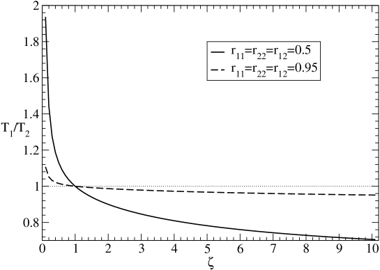
Figure 1: Temperature ratio as a function of the mass ratio for different choices of the inelasticity parameter, for $p=0.5$ and $r_{11}=r_{22}=r_{12}=r=0.8$ (solid line) and $r=0.5$ (dashed-line)

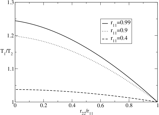
Figure 2: Temperature ratio as a function of the asymmetry $r_{22}/r_{11}$ for $p=0.5$, $\zeta=1$ and different choices of the inelasticity parameter $r_{11}$, from top to bottom this is respectively $0.99$, $0.9$, $0.4$ (line)

In fig. 2 the ratio of the temperatures of the two species is plotted in the case of an asymmetry in the restitution coefficients parametrized by the form: $r_{22}=r_{11}-x$ with $r_{12}=(r_{22}+r_{11})/2$, for $p=1/2$, identical masses and three different values of the coefficient $r_{11}$ as shown in figure. One sees that the variation of $\frac{T_{1}}{T_{2}}$ is much smaller than the corresponding variation with respect to the mass asymmetry shown in fig. 1 in agreement with the experimental observation of reference Menon . It seems reasonable to conclude that the mass asymmetry is the larger source of temperature difference between the two components.

IV Velocity distribution functions

An interesting aspect of granular systems concerns the nature of the single particle velocity distributions. The inelasticity, in fact, causes marked departures of $P_{\alpha}(v,t)$ from the Gaussian form which characterizes gases at thermal equilibrium. In undriven gases these deviations are particularly pronounced and one observes inverse power law high-velocity tails both in gases of pseudo-Maxwell molecules mixture and in IHS Ernst . In the driven case, i.e. in systems subject to Gaussian white noise forcing (similar to that represented by eq. (2) with $\Gamma=0$) exponential tails of the form $exp(-v^{3/2})$ have been predicted theoretically in inelastic hard-sphere models Ernst and tested by direct simulation Monte Carlo of the Enskog-Boltzmann equation Montanero . Have these non Gaussian tails a counterpart in Maxwell models? Ben-Naim and Krapivsky BenNaim on the basis of a re-summation of the moment expansion concluded that the scalar Maxwell models with vanishing viscosity ($\Gamma=0$) should display Gaussian-like tails. However, this prediction is in contrast with the argument, employed by Ernst and van Noije in the case of IHS, which consists in estimating the tails of the distribution by linearizing the master equation (9) by neglecting the gain term. This assumption simplifies the analysis and allows us to reach the conclusion that the velocity distribution for large $v$ should vanish as:

$$\lim_{v\to\infty}P(v)\propto\exp{(-v/v_{0})}$$ (20)

with $v_{0}^{2}=D\tau_{c}$. Clearly such a result is in sharp contrast with the result of ref. BenNaim and seems to indicate that the Sonine expansion does not reproduce faithfully the high-velocity tails in the case of Maxwell models with vanishing viscosity. The test of the limit (20) will be shown in the section 6, where we illustrate the results of our numerical simulations.

On the other hand, the same kind of asymptotic analysis sketched above, allows us to conclude that the presence of a viscous damping is the redeeming feature which renders convergent the Sonine expansion and the associated Gaussian tails. In fact, with a finite value of $\Gamma$ the asymptotic solution is of the form:

$$\lim_{v\to\infty}P(v)\propto\exp{(-Cv^{2})}$$ (21)

We shall test such a prediction in the remaining part of this section and study the velocity distributions of the individual species when $\Gamma\neq 0$ by constructing the solution to the master equation using the Sonine polynomial expansion method, one of the traditional approaches to the solution of the Boltzmann equation burnett .

We shall also investigate whether the two partial distributions can be cast into the same functional form upon re-scaling the velocities with respect to the partial granular thermal velocity, in other words if it is possible to have a data collapse for the two distributions.

We shall first obtain the steady state values of the first eight moments as illustrated in the Appendix and then compute the approximate form of the distribution functions by assuming that these are Gaussians multiplied by a linear combination of Sonine polynomials.

Let us begin by writing the following Sonine expansion of the distribution functions:

$$f_{\alpha}(c)=\frac{1}{\sqrt{\pi}}e^{-c^{2}}[1+\sum_{n=1}^{\infty}a^{\alpha}_{n}S_{n}(c^{2})]$$ (22)

where $f_{\alpha}(c)$ is the re-scaled distribution defined by:

$$f_{\alpha}(c)=\sqrt{2\mu^{\alpha}_{2}}P_{\alpha}(v).$$ (23)

and $c^{2}=v^{2}/2\mu^{\alpha}_{2}$. The expansion gives the distributions in terms of the coefficients $a^{\alpha}_{n}$ of the Sonine polynomials $S_{n}(c^{2})$. In practice, one approximates the series (22) with a finite number of terms. Since the leading term is the Maxwellian, the closer the system to the elastic limit, the less term suffice to describe the state. The expression of the first polynomials is:

$$S_{0}(c^{2}) =1$$ (24a)

$$S_{1}(c^{2}) =\frac{1}{2}-c^{2}$$ (24b)

$$S_{2}(c^{2}) =\frac{3}{8}-\frac{3}{2}c^{2}+\frac{1}{2}c^{4}$$ (24c)

$$S_{3}(c^{2}) =\frac{5}{16}-\frac{15}{8}c^{2}+\frac{5}{4}c^{4}-\frac{1}{6}c^{6}$$ (24d)

$$S_{4}(c^{2}) =\frac{35}{128}-\frac{35}{16}c^{2}+\frac{35}{16}c^{4}-\frac{7}{12}c^{6}+\frac{1}{24}c^{8}$$ (24e)

In order to obtain the first $m$ values $a^{\alpha}_{m}$, we need to compute the re-scaled moments $\langle c^{n}\rangle_{\alpha}$ of the distribution functions up to order $2m$. These moments are evaluated in Appendix by means of a straightforward iterative method. At the end, knowing the re-scaled moments, one obtains the following relation for the coefficients:

$$a^{\alpha}_{n}=\frac{\langle S_{n}(c^{2})\rangle_{\alpha}}{{\cal N}_{n}}$$ (25)

Eq. (25) can be proved by imposing the consistency condition:

$$\langle c^{n}\rangle_{\alpha}=\int_{-\infty}^{\infty}dcc^{n}f_{\alpha}(c)$$ (26)

in conjunction with the orthogonality property of the Sonine polynomials:

$$\int_{-\infty}^{\infty}\frac{1}{\sqrt{\pi}}e^{-c^{2}}S_{n}(c^{2})S_{m}(c^{2})={\cal N}_{n}\delta_{m,n}$$ (27)

where ${\cal N}_{n}$ is a normalization constant. Notice that in order to obtain our results we have not assumed weak inelasticity, therefore these hold for any value of the restitution coefficients.

The coefficients $a^{\alpha}_{m}$ up to the fourth order in terms of the re-scaled moments read:

$$a^{\alpha}_{1} =0$$ (28a)

$$a^{\alpha}_{2} =[1-4\langle c^{2}\rangle_{\alpha}+\frac{4}{3}\langle c^{4}\rangle_{\alpha}]$$ (28b)

$$a^{\alpha}_{3} =[1-6\langle c^{2}\rangle_{\alpha}+4\langle c^{4}\rangle_{\alpha}-\frac{8}{15}\langle c^{6}\rangle_{\alpha}]$$ (28c)

$$a^{\alpha}_{4} =[1-8\langle c^{2}\rangle_{\alpha}+8\langle c^{4}\rangle_{\alpha}-\frac{32}{15}\langle c^{6}\rangle_{\alpha}+\frac{16}{105}\langle c^{8}\rangle_{\alpha}]$$ (28d)

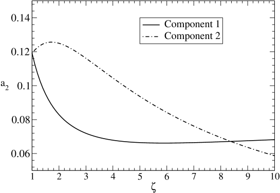
Figure 3: Second Coefficient of the Sonine expansion $a_{2}$, for each component as a function of the mass ratio $\zeta$, $m_{1}=1$ and for $p=0.5$ and $r_{11}=r_{22}=r_{12}=0.5$. We have also fixed $\frac{1}{\Gamma}\equiv\tau_{b1}=200$ and $\tau_{c}=25$.

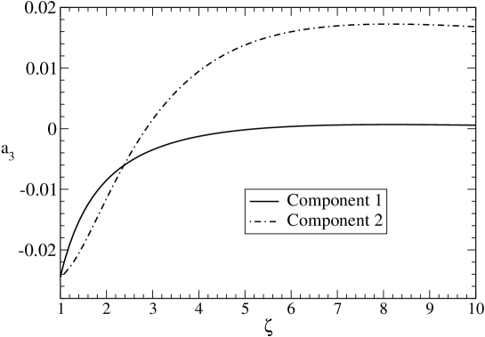
Figure 4: Third Coefficient of the Sonine expansion $a_{3}$, for each component as a function of the mass ratio $\zeta$. The remaining parameters as in fig. 3

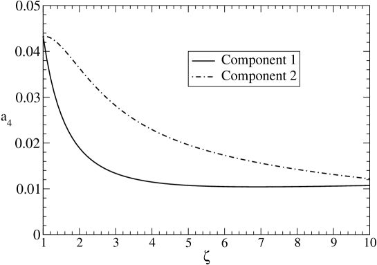
Figure 5: Fourth Coefficient of the Sonine expansion $a_{4}$, for each component as a function of the mass ratio $\zeta$. The remaining parameters as in fig. 3

In fig. (3-5) we display the behavior of the Sonine coefficients for both components in the case of equal restitution coefficients $r=0.5$ as a function of the mass ratio.

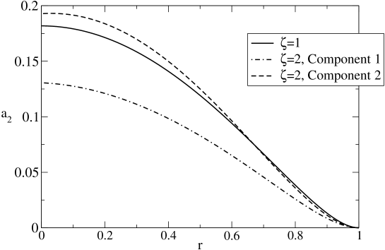
Figure 6: Second Coefficient of the Sonine expansion $a_{2}$, for each component as a function of the inelasticity $r=r_{11}=r_{22}=r_{12}$, for $p=0.5$ and $m_{1}=1$ and $\zeta=2$ and $\zeta=1$. The remaining parameters as in fig. 3.

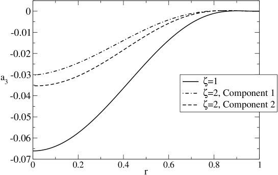
Figure 7: Third Coefficient of the Sonine expansion $a_{3}$, for each component as a function of the inelasticity $r=r_{11}=r_{22}=r_{12}$, for $p=0.5$ and $m_{1}=1$ and $\zeta=2$ and $\zeta=1$.The remaining parameters as in fig. 3.

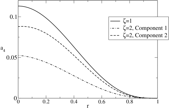
Figure 8: Fourth Coefficient of the Sonine expansion $a_{4}$, for each component as a function of the inelasticity $r=r_{11}=r_{22}=r_{12}$, for $p=0.5$ and $m_{1}=1$ and $\zeta=2$ and $\zeta=1$. The remaining parameters as in fig. 3.

In figs. (6-8) we illustrate the variation of the Sonine coefficients for the two components as a function of the inelasticity for two different values of the mass ratio: $\zeta=1$ and $\zeta=2$. Notice that the coefficients are monotonic functions of the inelasticity as already noticed in pure systems Ernst .

Figure 9: Rescaled distribution functions for the two components for a model system characterized by $m_{1}=1$, $m_{2}=0.5$ and equal inelasticities $r=0.5$.$T_{b}=1$ and the remaining parameters as in fig. 3

In fig.(9) we show the distribution functions for the heated system with non vanishing viscosity. The tails become fatter with increasing order of the approximation, i.e. the high energy tails are overpopulated. Moreover, one sees that when $p=1/2$ and the restitution coefficients are all equal the species with the larger tails is the lighter. On the other hand, for a system with the same masses, but different restitution coefficients, the more elastic species displays the larger tails. We also show the numerical data obtained by simulating the the dynamics. The agreement is quite satisfactory and validates the approximation method employed.

On the other hand, it is also evident, that the two distributions fail to collapse one over the other after the rescaling of the velocities. This fact is consistent with the different values assumed by the coefficients $a^{1}_{n}$ and $a^{2}_{n}$. However, this effect is rather small and can be appreciated only by studying the high velocity region of the distribution functions.

V Numerical Simulations

To investigate the validity of the previous results and in particular to test the convergence of the Sonine expansion in different situations we shall present in this section numerical results obtained by simulating an ensemble of $N$ particles subject to a Gaussian forcing, viscous friction and inelastic collisions.

The scheme consists of the following ingredients:

1. time is discretized, i.e. $t=n\cdot dt$

2. update all the velocities to simulate the random forcing and the viscous damping:

   $$v_{i}^{\alpha}(t+dt)=v_{i}^{\alpha}(t)e^{-\frac{dt}{\tau_{b}}}+\sqrt{T_{b}(1-e^{-\frac{2dt}{\tau_{b}}})}W(t)$$ (29)

   where $W(t)$ is a normally distributed deviate with zero mean and unit variance.

3. Choose randomly $N\frac{dt}{2\tau_{c}}$ pairs of velocities and update each of them with the collision rule (7). In this way a mean collision time $\tau_{c}$ per particle is guaranteed.

4. Change the time counter $n$ and restart from ii.

In other words, at every step each particle experiences a Gaussian kick thus receiving energy from the bath, whereas it dissipates energy by collision and by damping. For example, by choosing $dt=1$, $m_{1}/\Gamma=\tau_{b1}=200$ and $\tau_{c}=25$, we obtain that each particle in the average experiences $25$ Gaussian kicks between two successive collisions and that the resulting average kinetic energy is stationary. In order to compare our numerical simulations with the theoretical predictions we fixed the temperature of the bath to be $T_{b}=1$, i.e. chosen $D=\Gamma$. The results of such simulations are presented in fig. 9 and show a very good agreement between the theory and the simulation.

On the contrary, the agreement between the Sonine expansion and the simulation is not completely satisfactory when we consider a system subject to a white noise acceleration, but without viscous friction, a driving proposed by some authors Peng , Moon . This can be considered as the limit $\Gamma\to 0$, $T_{b}\to\infty$, keeping constant $D=T_{b}\Gamma$, in the model defined by eqs. (8): note that in this case the elastic limit $r\to 1$ cannot be performed without taking also the limit $D\to 0$ as discussed at the beginning, in order to avoid a divergence of kinetic energy. For the sake of simplicity, we simulated a one component system ($p=1$ and $m=1$) with vanishing viscosity $\Gamma=0$, but $D=0.0008$, $\tau_{c}=250$ and $r=0.5$. Such a choice yields a granular temperature $T_{g}=16/15$, as predicted by our formula (18). Notice that in this case the heath bath temperature diverges and the gas does not have a proper elastic limit, since all moments diverge when $\gamma\to 0$. We observed that the tails of the velocity distribution function are strongly non Gaussian. These decay as a simple exponential as predicted by our simple analysis of the previous section. In fig. (9) we report our simulation results against the Sonine approximation. We observe that the theoretical estimate, in spite of incorporating the exact values of the first eight moments, deviates from the numerical data in the large velocity region. In particular the Sonine expansion can only give Gaussian tails, whereas the simulation indicates a slower exponential decay. The reason for such a discrepancy is to be ascribed to the slow convergence of the expansion when $\Gamma=0$.

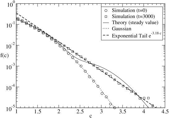
Figure 10: Rescaled distribution functions for a one component system ($p=1$) with vanishing viscosity ($\Gamma=0$), $D=0.0008$ , $r=0.5$ and $\tau_{c}=250$. We show the initial Gaussian distribution ($t=0$) and the asymptotic ($t=3000$) stationary distribution. Notice the presence of high velocity tails. For the sake of comparison we report the theoretical estimate of the distribution obtained by means of the Sonine expansion.

VI Discussion and Conclusions

To summarize we have studied the behavior of a model, which perhaps represent the simplest description of a driven inelastic gas mixture, namely an assembly of two types of scalar pseudo-Maxwell molecules subject to a stochastic forcing. We have obtained the velocity distributions for arbitrary values of the inelasticity, of the composition and of the masses by solving the associated Boltzmann equation by means of a controlled approximation, the moment expansion. The distributions were obtained by computing exactly the moments up to the eighth order and then imposing that the corrections to the Maxwell distribution stemming from the inelasticity are Gaussians multiplied by a linear combination of Sonine polynomials with amplitudes determined self-consistently.

The model predicts a steady two temperature behavior which is in qualitative agreement with existing experimental results. The granular temperatures can be obtained by very simple algebraic manipulations for arbitrary values of the control parameters.

By numerical simulations we demonstrated that the velocity distributions are well described by our series representation in the case of systems in contact with a bath at finite temperature $T_{b}$, whilst the series expansion breaks down in the case of systems in contact with bath at infinite temperature, i.e. with zero viscosity.

What can be learned from such a simple model of granular mixture? Besides obtaining a global picture of the behavior of the system with a minimal numerical effort both in the cooling and in the driven case, the model displays the novel feature of two different distribution functions, which remain different even after rescaling by the associated partial granular temperatures. Of course the detailed form of the probability velocity distributions are strictly model dependent, i.e. depend on the assumption of a constant collision rate inherent in Maxwell models. Finally, the vectorial character of the velocities could be included at the cost of a moderate additional effort. A more interesting and difficult problem would be that of including in the mixture case a collision frequency proportional to an appropriate function of the kinetic granular temperatures, generalizing the work of Cercignani Cercignani .

Finally we might ask the general question of the meaning of granular temperature. Our findings seem to indicate that it is still the main statistical indicator of the model granular system we studied. However, with respect to the temperature of a perfectly elastic system it fails to satisfy a very basic requirement which is known as the zeroth principle of thermodynamics.

*

Appendix A

In the present Appendix we sketch the derivation of the various moments of the distribution functions. By equating the equal powers of $k$ in the master equation (11) we obtain a set linear of coupled equations for the moments. The method of solution is iterative, because the higher moments depend on the lower moments. Thus, for instance, to evaluate the lowest order moments of the distribution functions we must solve the following equations for the steady state value of the fourth moments:

$$(d^{(4)}_{11}-4\Gamma_{1}\tau_{c})\mu^{(1)}_{4}+d^{(4)}_{12}\mu^{(2)}_{4}+a_{11}(\mu^{(1)}_{2})^{2}+a_{12}\mu^{(1)}_{2}\mu^{(2)}_{2}+12D_{1}\tau_{c}\mu^{(1)}_{2} =0$$ (30a)

$$(d^{(4)}_{22}-4\Gamma_{2}\tau_{c})\mu^{(2)}_{4}+d^{(4)}_{21}\mu^{(1)}_{4}+a_{22}(\mu^{(2)}_{2})^{2}+a_{21}\mu^{(1)}_{2}\mu^{(2)}_{2}+12D_{2}\tau_{c}\mu^{(2)}_{2} =0$$ (30b)

In turn, the sixth moments are obtained by solving:

$$(d^{(6)}_{11}-6\Gamma_{1}\tau_{c})\mu^{(1)}_{6}+d^{(6)}_{12}\mu^{(2)}_{6}+b_{11}\mu^{(1)}_{2}\mu^{(1)}_{4}+b_{12}\mu^{(1)}_{2}\mu^{(2)}_{4}+b_{12}^{\prime}\mu^{(2)}_{2}\mu^{(1)}_{4}+30D_{1}\tau_{c}\mu^{(1)}_{4} =0$$ (31a)

$$(d^{(6)}_{22}-6\Gamma_{2}\tau_{c})\mu^{(2)}_{6}+d^{(6)}_{21}\mu^{(1)}_{6}+b_{22}\mu^{(2)}_{2}\mu^{(2)}_{4}+b_{21}\mu^{(1)}_{2}\mu^{(2)}_{4}+b_{21}^{\prime}\mu^{(2)}_{2}\mu^{(1)}_{4}+30D_{2}\tau_{c}\mu^{(2)}_{4} =0$$ (31b)

Finally the eight moments are the solutions of:

$$\begin{split}(d^{(8)}_{11}-8\Gamma_{1}\tau_{c})\mu^{(1)}_{8}&+d^{(8)}_{12}\mu^{(2)}_{8}+c_{11}\mu^{(1)}_{2}\mu^{(1)}_{6}+c_{11}^{\prime}(\mu^{(1)}_{4})^{2}\\ &+c_{12}\mu^{(1)}_{2}\mu^{(2)}_{6}+c_{12}^{\prime}\mu^{(1)}_{4}\mu^{(2)}_{4}+c_{12}^{\prime\prime}\mu^{(1)}_{6}\mu^{(2)}_{2}+56D_{1}\tau_{c}\mu^{(1)}_{6}=0\end{split}$$ (32a)

$$\begin{split}(d^{(8)}_{22}-8\Gamma_{2}\tau_{c})\mu^{(2)}_{8}&+d^{(8)}_{21}\mu^{(1)}_{8}+c_{22}\mu^{(2)}_{2}\mu^{(2)}_{6}+c_{22}^{\prime}(\mu^{(2)}_{4})^{2}\\ &+c_{21}\mu^{(2)}_{2}\mu^{(1)}_{6}+c_{21}^{\prime}\mu^{(2)}_{4}\mu^{(1)}_{4}+c_{21}^{\prime\prime}\mu^{(2)}_{6}\mu^{(1)}_{2}+56D_{2}\tau_{c}\mu^{(2)}_{6}=0\end{split}$$ (32b)

where the general form of the coefficients $d_{ij}$ is given by:

$$d^{(n)}_{11} =-1+p[\gamma_{11}^{n}+(1-\gamma_{11})^{n}]+(1-p)[\tilde{\gamma}_{12}]^{n}$$ (33a)

$$d^{(n)}_{12} =(1-p)[(1-\tilde{\gamma}_{12})]^{n}$$ (33b)

$$d^{(n)}_{22} =-1+(1-p)[\gamma_{22}^{n}+(1-\gamma_{22})^{n}]+p[\tilde{\gamma}_{21}]^{n}$$ (33c)

$$d^{(n)}_{21} =p[(1-\tilde{\gamma}_{21})]^{n}$$ (33d)

and the coefficients $a_{ij}$ are given by:

$$a_{11} =6p[\gamma_{11}(1-\gamma_{11})]^{2}$$ (34a)

$$a_{22} =6(1-p)[\gamma_{22}(1-\gamma_{22})]^{2}$$ (34b)

$$a_{12} =6(1-p)[(1-\tilde{\gamma}_{12})]^{2}[\tilde{\gamma}_{12})]^{2}$$ (34c)

$$a_{21} =6p[(1-\tilde{\gamma}_{21})]^{2}[\tilde{\gamma}_{21})]^{2}$$ (34d)

Finally, the coefficients $b_{ij}$ are given by:

$$b_{11} =15p\gamma_{11}^{2}(1-\gamma_{11})^{2}[\gamma_{11}^{2}+(1-\gamma_{11})^{2}]$$ (35a)

$$b_{22} =15(1-p)\gamma_{22}^{2}(1-\gamma_{22})^{2}[\gamma_{22}^{2}+(1-\gamma_{22})^{2}]$$ (35b)

$$b_{12} =15(1-p)[(1-\tilde{\gamma}_{12})]^{4}[\tilde{\gamma}_{12})]^{2}$$ (35c)

$$b^{\prime}_{12} =15(1-p)[(1-\tilde{\gamma}_{12})]^{2}[\tilde{\gamma}_{12})]^{4}$$ (35d)

$$b_{21} =15p[(1-\tilde{\gamma}_{21})]^{2}[\tilde{\gamma}_{21})]^{4}$$ (35e)

$$b^{\prime}_{21} =15p[(1-\tilde{\gamma}_{21})]^{4}[\tilde{\gamma}_{21})]^{2}$$ (35f)

and $c_{ij}$ are

$$c_{11} =28p\gamma_{11}^{2}(1-\gamma_{11})^{2}[\gamma_{11}^{4}+(1-\gamma_{11})^{4}]$$ (36a)

$$c_{11}^{\prime} =70p\gamma_{11}^{4}(1-\gamma_{11})^{4}$$ (36b)

$$c_{12} =28(1-p)[(1-\tilde{\gamma}_{12})]^{6}[\tilde{\gamma}_{12})]^{2}$$ (36c)

$$c_{12}^{\prime} =70(1-p)[(1-\tilde{\gamma}_{12})]^{4}[\tilde{\gamma}_{12})]^{4}$$ (36d)

$$c_{12}^{\prime\prime} =28(1-p)[(1-\tilde{\gamma}_{12})]^{2}[\tilde{\gamma}_{12})]^{6}$$ (36e)

$$c_{22} =28(1-p)\gamma_{22}^{2}(1-\gamma_{22})^{2}[\gamma_{22}^{4}+(1-\gamma_{22})^{4}]$$ (36f)

$$c_{22}^{\prime} =70(1-p)\gamma_{22}^{4}(1-\gamma_{22})^{4}$$ (36g)

$$c_{21} =28p[(1-\tilde{\gamma}_{21})]^{6}[\tilde{\gamma}_{21})]^{2}$$ (36h)

$$c_{21}^{\prime} =70p[(1-\tilde{\gamma}_{21})]^{4}[\tilde{\gamma}_{21})]^{4}$$ (36i)

$$c_{21}^{\prime\prime} =28p[(1-\tilde{\gamma}_{21})]^{2}[\tilde{\gamma}_{21})]^{6}$$ (36j)

It is useful to consider the behavior of the moments in the one component case. The major simplicity of the resulting formulae allows us to obtain explicit expressions:

$$\mu_{2} =\frac{D\tau_{c}}{\Gamma\tau_{c}+\gamma(1-\gamma)}$$ (37a)

$$\mu_{4} =\frac{12D\tau_{c}\mu_{2}+6\gamma^{2}(1-\gamma)^{2}\mu_{2}^{2}}{4\Gamma\tau_{c}+1-\gamma^{4}-(1-\gamma)^{4}}$$ (37b)

$$\mu_{6} =\frac{30D\tau_{c}\mu_{4}+15\gamma^{2}(1-\gamma)^{2}(\gamma^{2}+(1-\gamma)^{2}\mu_{2}\mu_{4}}{6\Gamma\tau_{c}+1-\gamma^{6}-(1-\gamma)^{6}}$$ (37c)

$$\mu_{8} =\frac{56D\tau_{c}\mu_{6}+28\gamma^{2}(1-\gamma)^{2}(\gamma^{4}+(1-\gamma)^{4})\mu_{2}\mu_{6}+70\gamma^{4}(1-\gamma)^{4}\mu_{4}^{2}}{8\tau_{c}\Gamma+1-\gamma^{8}-(1-\gamma)^{8}}$$ (37d)

References

- (1) H.M. Jaeger, S.R. Nagel and R.P. Behringer, Rev. Mod. Phys. 68, 1259 (1996).
- (2) K.Feitosa and N.Menon, cond-mat/0111391 (2001)
- (3) A.B.Pippard, “The Elements of Classical Thermodynamics”, Cambridge University Press (Cambridge) (1957).
- (4) V.Garzó and J.Dufty, Phys.Rev. E 60, 5706 (1999).
- (5) C. S. Campbell, Annu. Rev. Fluid Mech. 22, 57 (1990).
- (6) M.H. Ernst, Phys.Reports 78, 1 (1981).
- (7) E.Ben-Naim and P.L. Krapivsky, Phys.Rev. E 61, R5 (2000).
- (8) P.L. Krapivsky and E.Ben-Naim, cond-mat/0111044 (2001).
- (9) A.Baldassarri, U. Marini Bettolo Marconi and A. Puglisi, to appear in Europhys.Lett. cond-mat/0105299 (2001)
- (10) A.Baldassarri, U. Marini Bettolo Marconi and A. Puglisi, subm. for publication cond-mat/0111066 (2001)
- (11) U. Marini Bettolo Marconi, A. Baldassarri and A. Puglisi, Advances in Complex Systems 4, 321 (2001).
- (12) M.H. Ernst and R. Brito, cond-mat/0112417 (2001).
- (13) J.A. Carrillo, C.Cercignani and I.M. Gamba, Phys. Rev. E 62, 7700 (2000).
- (14) A.V. Bobylev, J.A. Carrillo and I.M. Gamba, J.Stat.Phys. 98, 743 (2000)
- (15) A.Puglisi, V.Loreto,U. Marini Bettolo Marconi, A. Petri and A.Vulpiani, Phys.Rev.Lett 81, 3848 (1998) and A.Puglisi, V.Loreto,U. Marini Bettolo Marconi, A. Petri and A.Vulpiani, Phys.Rev. E 59, 5582 (1999).
- (16) Notice that, in order to reduce the number of free parameters, we have assumed the constants, and , which specify the interactions with the bath to be species independent. Such a choice implies that in the elastic limit both components reach the same granular temperature given by the temperature of the bath .
- (17) A.V.Bobylev, Sov. Phys.Dokl. 20, 820 (1976).
- (18) U. Marini Bettolo Marconi and A. Puglisi, submitted for publication, cond-mat/0112336 (2001)
- (19) T.P.C. van Noije and M.H. Ernst, Granular Matter 1, 57 (1998).
- (20) J.M. Montanero and A. Santos, Granular Matter 2, 53 (2000).
- (21) D. Burnett, Proc.London Math. Soc. 40, 382 (1935).
- (22) G.Peng and T.Ohta, Phys.Rev. E 58, 4737 (1998).
- (23) S.J. Moon, M.D. Shattuck and J.B. Swift, Phys.Rev. E 64, 031303 (2001).