MMM2D: A fast and accurate summation method for electrostatic interactions in 2D slab geometries

Abstract

We present a new method, in the following called MMM2D, to accurately calculate the electrostatic energy and forces on charges being distributed in a two dimensional periodic array of finite thickness. It is not based on an Ewald summation method and as such does not require any fine-tuning of an Ewald parameter for convergence. We transform the Coulomb sum via a convergence factor into a series of fast decaying functions which can be easily evaluated. Rigorous error bounds for the energies and the forces are derived and numerically verified. Already for small systems our method is much faster than the traditional $2D$–Ewald methods, but for large systems it is clearly superior because its time demand scales like ${\mathcal{O}}(N^{5/3})$ with the number $N$ of charges considered. Moreover it shows a rapid convergence, is very precise and easy to handle.

,

1 Introduction

The calculation of Coulomb interactions are time consuming due to their long range nature. In principle, each charge $q_{i}$ at position $p_{i}$ interacts with all others, leading to a computational effort of ${\mathcal{O}}(N^{2})$ already within the central simulation box. For many physical investigations one wants to simulate bulk properties and therefore introduces periodic boundary conditions to avoid surface effects. The Coulomb energy $E$ then has to be computed as a sum over all periodic images,

$$E=\frac{1}{2}\sideset{}{{}^{\prime}}{\sum}_{n\in\mathbb{Z}^{3}}\sum_{i,j}\frac{q_{i}q_{j}}{|p_{i}-p_{j}+n\lambda|},$$ (1)

where for simplicity we assume a cubic simulation box of length $\lambda$. The prime denotes that for $n=0$ the term $i=j$ has to be omitted. This sum is merely conditionally convergent, meaning that its value depends on the summation order. Normally a spherical limit is used, i. e. the vectors $n$ are added in the order of increasing length. Then $E$ can be computed for example via the traditional Ewald summation method [1]. The basic idea of this method is to split the original sum via a simple transformation involving the splitting parameter $\alpha$ into two exponentially convergent parts, where the first one is short ranged and evaluated in real space, the other one is long ranged and can be analytically Fourier transformed and evaluated in Fourier space. For any choice of the Ewald parameter $\alpha$ and no truncation in the sums the formula yields the exact result. In practice one cuts off the infinite sums at some finite values and obtains $E$ to a user controlled accuracy, which is possible by using error estimates for the cut-offs [2].

Another way of computing Eq. (1) is via a convergence factor

$$\tilde{E}=\lim_{\beta\rightarrow 0}\frac{1}{2}\sideset{}{{}^{\prime}}{\sum}_{n\in\mathbb{Z}^{3}}\sum_{ij}\frac{q_{i}q_{j}\exp{(-\beta|p_{i}-p_{j}+n\lambda|)}}{|p_{i}-p_{j}+n\lambda|}.$$ (2)

This approach is used in a method due to Sperb [3] called MMM.

In Refs.[4, 5] it was shown that Eqs. (1) and (2) differ by a term proportional to the dipole moment for 3D systems. Sperb et al. have developed a factorization approach which yields an ${\mathcal{O}}(N\log N)$ algorithm [6], comparable in speed to the FFT mesh based Ewald algorithms[7, 8]. An different convergence factor was used by Lekner [9] to efficiently sum up the 3D Coulomb sum. But this approach still leads to an ${\mathcal{O}}(N^{2})$ algorithm.

For thin polyelectrolytes films, membrane interactions, or generally confined charged systems, one is interested in summations where only 2 dimensions are periodically replicated and the third one (here always the z-direction) is of finite thickness $h$ ($2D+h$ geometry). For this geometry Ewald based formulas are only slowly convergent, have mostly ${\mathcal{O}}(N^{2})$ scalings and no “a priori” error estimates exist [10]. In Ref.[10] a comparison was made with respect to speed and accuracy of the three most popular versions, the traditional $2d$–Ewald method developed by Heyes, Barber, and Clarke (HBC) [11], the one due to Hautmann-Klein (HK) [12], and the approach attributed to Nijboer and de Wette (NdW) [13, 14]. Another variant is due to Smith [15], which combines HBC and NdW, resulting in a good scaling, but still slow convergence. Recently two more Ewald-type methods were proposed with different ways of approximating the Fourier space sum of the HBC-formula[16, 17].

The aim of this paper is to develop a new method, which we call MMM2D. A brief description of the key features of this algorithm was already given in Ref.[18]. MMM2D will be using the same ideas leading to MMM and is therefore derived from an equation like Eq. (2) using a convergence factor. We will show that for two dimensional systems this approach yields the same results as the spherical limit, i. e. $E=\tilde{E}$. In principle, already the 3D formula developed by Lekner [19] could be used for 2D + h Systems. It employs modified Bessel functions, but is only useful for particles separated in the $z$–direction, and is only calculable pairwise. Sperb [20] derived a different formula, which is also applicable for particles lying in the same $z$–plane. A combination of theses two formula has been used recently in MD simulations, because it is easy to implement [21] for small number of particles, but suffers the drawback of being an ${\mathcal{O}}(N^{2})$ method, and therefore the system sizes which can be investigated are limited. Moreover these methods use different convergence factors, and up to now no investigations have been performed to see whether both methods lead to the same result as the one obtained by using a spherical limit.

To precisely define the problem we consider systems of $N$ particles with charges $q_{i}\in\mathbb{R}$ and pairwise different coordinates $p_{i}=(x_{i},y_{i},z_{i})^{T}\in B_{0}$, $i=1,\ldots,N$, where

$$B_{0}=\biggl{(}-\frac{\lambda_{x}}{2},\frac{\lambda_{x}}{2}\biggr{]}\times\biggl{(}-\frac{\lambda_{y}}{2},\frac{\lambda_{y}}{2}\biggr{]}\times\mathbb{R}\subset\mathbb{R}^{3}$$

is the simulation box. Furthermore it is assumed that the system is charge neutral, i. e. $\sum_{i=1}^{N}q_{i}=0$.

Now let $n_{kl}:=(k\lambda_{x},l\lambda_{y},0)^{T}$ for $k,l\in\mathbb{Z}$. The expressions to be calculated are the interaction energies of particle $i$ with all other charges, defined as

$$E_{i}=\sum_{S=0}^{\infty}\sum_{\begin{subarray}{c}k,l\in\mathbb{Z},\\ k^{2}+l^{2}=S\end{subarray}}\sideset{}{{}^{\prime}}{\sum}_{j=1}^{N}\frac{q_{i}q_{j}}{|p_{i}-p_{j}+n_{kl}|}\quad i=1\ldots N\,\text{.}$$ (3)

As usual the prime ^′ on the inner sum indicates that the term $j=i$ for $k=l=0$ is omitted.

In Sec. 2 we will develop the formulas used by MMM2D for calculating the energy and the forces. In Sec. 3 we develop error formulas for the energy and force calculations, which can be easily calculated prior to a simulation. Then, in Sec. 4 we give the details of our implementation, which is based on a factorization approach resulting in an ${\mathcal{O}}(N^{5/3})$ scaling. In Sec. 5 we apply our algorithm to several test cases and prove its applicability and efficiency. We will also demonstrate that it is much faster than the $2d$–Ewald method, and is thus a superior alternative to all aforementioned methods. We will end with some conclusions, and show for the interested reader in the Appendix A that for two dimensional systems $E=\tilde{E}$, i. e. that the summation using a convergence factor as in Eq. (2) yields exactly the same result as the summation using a spherical limit as the $2d$–Ewald method, there is no dipolar correction term needed.

2 The MMM2D Method

The transformations given here are similar to the transformations used in R. Strebel’s MMM [22, 6] for three–dimensional periodic systems. The ideas used in the following are similar to the ideas used to develop the formulas for MMM. Basically, two different formulas are used to calculate the energy and forces. For the interaction between particles that are well separated, a formula that can be calculated in linear time is used. For the interaction between neighboring particles a second formula is used. This leads to an ${\mathcal{O}}(N^{7/5})$ algorithm. Up to here the same ideas are used for MMM2D. But for the three dimensional case some further tricks are used to achieve the scaling of ${\mathcal{O}}(N\log N)$. These tricks involve the symmetry of the coordinates which is not true for two dimensional systems. Therefore this better scaling cannot be carried over to the two dimensional case.

The formulas needed for MMM2D are derived in the next subsections in the same way as has been done for MMM[22]. We first rewrite the sum (3) using a convergence factor:

$$E_{i}=\,\lim_{\beta\rightarrow 0}\sum_{k,l\in\mathbb{Z}}\sideset{}{{}^{\prime}}{\sum}_{j=1}^{N}\frac{q_{i}q_{j}e^{-\beta|p_{ij}+n_{kl}|}}{|p_{ij}+n_{kl}|}=\,\lim_{\beta\rightarrow 0}\sum_{j=1}^{N}q_{i}q_{j}\phi_{\beta}(x_{ij},y_{ij},z_{ij})$$ (4)

where $p_{ij}=(x_{ij},y_{ij},z_{ij})=p_{i}-p_{j}$,

$$\phi_{\beta}(x,y,z)=\,\tilde{\phi}_{\beta}(x,y,z)+\begin{cases}\frac{e^{-\beta r}}{r}&(x,y,z)\neq(0,0,0)\\ 0&(x,y,z)=(0,0,0)\end{cases}$$ (5)

and

$$\begin{split}\tilde{\phi}_{\beta}(x,y,z)=\,&\sum_{(k,l)\neq(0,0)}\frac{e^{-\beta r_{kl}}}{r_{kl}}\end{split}\,\text{,}$$ (6)

where we abbreviated

$$r_{kl}=\sqrt{(x+k\lambda_{x})^{2}+(y+l\lambda_{y})^{2}+z^{2}}\,\text{,}\quad r_{k}=r_{k0}\,\text{,}\quad r=r_{0}\,\text{.}$$

The fact that the rhs. of Eq. (4) is equal to Eq. (3) is non–trivial; see appendix A for a proof.

2.1 Transformation of $\phi_{\beta}$ for $z\neq 0$

First we concentrate on developing an absolutely and rapidly converging formula for $\phi_{\beta}$. Then we can easily form the limit $\beta\rightarrow 0$ and obtain a formula for $\phi$. For $z\neq 0$ and $\beta>0$ the sum in $\phi_{\beta}$ is an absolutely convergent sum of Schwartz class functions. Therefore for $\delta>0$ and $x\in\mathbb{R}$, we can apply the Poisson formula:

$$\sum_{k\in\mathbb{Z}}f(x+\delta k)=\frac{1}{|\delta|}\sum_{p\in\mathbb{Z}}{\mathcal{F}}(f)\left(\frac{p}{\delta}\right)e^{2\pi i\frac{p}{\delta}x}\,\text{,}$$ (7)

where ${\mathcal{F}}$ denotes the Fourier transformation. Furthermore we will be using the formulas

$${\mathcal{F}}\left(\frac{e^{-\beta\sqrt{\alpha^{2}+\cdot\,^{2}}}}{\sqrt{\alpha^{2}+\cdot\,^{2}}}\right) =2\operatorname{K}_{0}\left(\alpha\sqrt{\beta^{2}+(2\pi\,\cdot)^{2}}\right)\,\text{,}$$

$${\mathcal{F}}\left(\operatorname{K}_{0}\left(\alpha\sqrt{z^{2}+\cdot\,^{2}}\right)\right) =\pi\frac{e^{-z\sqrt{\alpha^{2}+(2\pi\,\cdot)^{2}}}}{\sqrt{\alpha^{2}+(2\pi\,\cdot)^{2}}}$$

which are valid for $\alpha,z\in\mathbb{R}$ and can be found, for example, in [23]. $\operatorname{K}_{0}$ is called the modified Bessel function of order 0. For properties of the Bessel functions, see [24].

Setting

$$\beta_{pq}=\sqrt{\beta^{2}+(2\pi u_{x}p)^{2}+(2\pi u_{y}q)^{2}}\,\text{,}$$

$$\beta_{p}=\sqrt{\beta^{2}+(2\pi u_{x}p)^{2}}\quad\text{and}\quad\beta_{q}=\sqrt{\beta^{2}+(2\pi u_{y}q)^{2}}\,\text{,}$$

$$\rho_{l}=\sqrt{(y+l\lambda_{y})^{2}+z^{2}}\,\text{,}\quad\rho=\rho_{0}\,\text{,}\quad u_{x}=\frac{1}{\lambda_{x}}\quad\text{and}\quad u_{y}=\frac{1}{\lambda_{y}}\,\text{.}$$

we obtain after two Fourier transformations

$$\begin{split}\phi_{\beta}(x,y,z)&=\,\sum_{k,l\in\mathbb{Z}}\frac{e^{-\beta r_{kl}}}{r_{kl}}=\,\sum_{l\in\mathbb{Z}}\left(\sum_{k\in\mathbb{Z}}\frac{e^{-\beta r_{kl}}}{r_{kl}}\right)\\ &=\,2u_{x}\sum_{p\in\mathbb{Z}}\left(\sum_{l\in\mathbb{Z}}\operatorname{K}_{0}\left(\beta_{p}\rho_{l}\right)\right)e^{2\pi iu_{x}px}\\ &=\,2\pi u_{x}u_{y}\sum_{p,q\in\mathbb{Z}}\frac{e^{-\beta_{pq}|z|}}{\beta_{pq}}e^{2\pi iu_{x}px}e^{2\pi iu_{y}qy}\,\text{.}\end{split}$$

Expanding the term for $p=q=0$ we find $\frac{e^{-\beta|z|}}{\beta}=\beta^{-1}-|z|+\underset{\beta\rightarrow 0}{\mathcal{O}}(\beta)$, and obtain our final formula

$$\begin{split}&\phi_{\beta}(x,y,z)=\,8\pi u_{x}u_{y}\sum_{p,q>0}\frac{e^{-\beta_{pq}|z|}}{\beta_{pq}}\cos(2\pi u_{x}px)\cos(2\pi u_{y}qy)\,+\\ &\quad 4\pi u_{x}u_{y}\sum_{q>0}\frac{e^{-\beta_{q}|z|}}{\beta_{q}}\cos(2\pi u_{y}qy)\,+4\pi u_{x}u_{y}\sum_{p>0}\frac{e^{-\beta_{p}|z|}}{\beta_{p}}\cos(2\pi u_{x}px)\,-\\ &\quad 2\pi u_{x}u_{y}|z|+2\pi u_{x}u_{y}\beta^{-1}+\underset{\beta\rightarrow 0}{\mathcal{O}}(\beta)\,\text{.}\end{split}$$ (8)

It has a singularity of $2\pi u_{x}u_{y}\beta^{-1}$ which is independent of the particle coordinates. However, once the sum of $\phi_{\beta}$ is taken over all particles, the singularity vanishes via the charge neutrality condition. For the other parts of Eq. (8) taking the limit $\beta\rightarrow 0$ is trivial. The resulting formula (see Sec. 2.3) can be evaluated linearly in time, just like the Fourier part of the Ewald sum. This will be shown in more detail in section 4.

Unfortunately the convergence becomes slower with decreasing $z$ and for $z=0$ the sum is not defined. Thus we will need an alternative method for small $z$.

2.2 Transformation of $\tilde{\phi}_{\beta}$ for $z\approx 0$

For small particle distances, the term for $k=l=0$ is dominant (and must be omitted for the interaction of a particle with its own images). Therefore we leave it out for now and concentrate on a rapidly convergent formula for $\tilde{\phi}_{\beta}(x,y,z)$. This requires a little more work. For a more detailed derivation see [22, 25].

Since we omit the $k=l=0$ term, the area to sum over has a hole. To efficiently treat the sum over this area we split $\tilde{\phi}_{\beta}(x,y,z)=\Sigma_{1}+\Sigma_{2}$ where

$$\Sigma_{1}=\sum_{l\neq 0}\sum_{k\in\mathbb{Z}}\frac{e^{-\beta r_{kl}}}{r_{kl}}\quad\text{and}\quad\Sigma_{2}=\sum_{k\neq 0}\frac{e^{-\beta r_{k0}}}{r_{k0}}\,\text{.}$$

Graphically this can be displayed like that:

We start by calculating $\Sigma_{1}$. Using the same argument as for formula (8) we obtain

$$\begin{split}\Sigma_{1}&=\,\sum_{l\neq 0}\sum_{k\in\mathbb{Z}}\frac{e^{-\beta r_{kl}}}{r_{kl}}=\,2u_{x}\sum_{l\neq 0}\sum_{p\in\mathbb{Z}}\operatorname{K}_{0}(\beta_{p}\rho_{l})e^{2\pi iu_{x}px}\\ &=\,2u_{x}\sum_{l,p\neq 0}\operatorname{K}_{0}(\beta_{p}\rho_{l})e^{2\pi iu_{x}px}+2u_{x}\sum_{l\neq 0}\operatorname{K}_{0}(\beta\rho_{l})\,\text{.}\end{split}$$

While the first sum converges fast, the second one is still singular in $\beta$ and has to be investigated further:

$$\begin{split}2u_{x}\sum_{l\neq 0}\operatorname{K}_{0}(\beta\rho_{l})&=\,2u_{x}\sum_{l\in\mathbb{Z}}\operatorname{K}_{0}(\beta\rho_{l})-2u_{x}\operatorname{K}_{0}(\beta\rho)\\ &=\,2u_{x}\sum_{l\in\mathbb{Z}}\operatorname{K}_{0}(\beta\rho_{l})-2u_{x}(\log 2-\gamma-\log(\beta\rho))+\underset{\beta\rightarrow 0}{\mathcal{O}}(\beta^{2})\end{split}$$

where we have used the asymptotic behavior $\operatorname{K}_{0}(x)=-\log\frac{x}{2}-\gamma+{\mathcal{O}}(x^{2})$ for $x\rightarrow 0$.

The first sum can now be Fourier transformed again:

$$\begin{split}\sum_{l\in\mathbb{Z}}\operatorname{K}_{0}(\beta\rho_{l})&=\,\pi u_{y}\sum_{q>0}\frac{e^{-\beta_{q}|z|}}{\beta_{q}}\left(e^{2\pi iu_{y}qy}+e^{-2\pi iu_{y}qy}\right)+\pi u_{y}\frac{e^{-\beta|z|}}{\beta}\\ &=\,2\pi u_{y}\operatorname{Re}\left(\sum_{q>0}\frac{e^{-2\pi u_{y}q|z|}}{2\pi u_{y}q}e^{2\pi iu_{y}qy}\right)+\pi u_{y}(\beta^{-1}-|z|)+\underset{\beta\rightarrow 0}{\mathcal{O}}(\beta)\,\text{.}\end{split}$$

If we set $\zeta:=2\pi u_{y}(|z|+iy)$, we obtain

$$\begin{split}2\pi u_{y}\sum_{q>0}\frac{e^{-2\pi u_{y}q|z|}}{2\pi u_{y}q}e^{2\pi iu_{y}qy}&=\,\sum_{q>0}\frac{e^{-q\zeta}}{q}=\,-\log(\zeta)+\frac{\zeta}{2}-\sum_{n\geq 2}\frac{b_{n}}{n\,n!}\zeta^{n}\end{split}$$

where $b_{n}$ are the Bernoulli numbers. This series expansion is valid only for $|\zeta|\leq 2\pi$, which is fulfilled if $|z|\leq\frac{\lambda_{y}}{2}$. The last equality is found by integration from

$$\begin{split}&\frac{d}{dz}\log\left(\frac{1-e^{-z}}{z}\right)=z^{-1}\left(\frac{z}{e^{z}-1}-1\right)\\ &\quad=z^{-1}\left(\sum_{n=0}^{\infty}\frac{b_{n}}{n!}z^{n}-1\right)=-\frac{1}{2}+\sum_{n=1}^{\infty}\frac{b_{2n}}{(2n)!}z^{2n-1}\,\text{,}\end{split}$$

where the defining series $\frac{z}{e^{z}-1}=\sum_{n=0}^{\infty}\frac{b_{n}}{n!}z^{n}$ for the Bernoulli numbers was used.

Using $\operatorname{Re}(-\log\zeta)=-\log|\zeta|=-\log(2\pi u_{y}\rho)$ and $\operatorname{Re}\left(\frac{\zeta}{2}\right)=\pi u_{y}|z|$ we obtain

$$\begin{split}\sum_{l\in\mathbb{Z}}\operatorname{K}_{0}(\beta\rho_{l})=\,&-\sum_{n\geq 2}\frac{b_{n}}{n\,n!}\operatorname{Re}\left(\zeta^{n}\right)-\log(2\pi u_{y}\rho)+\pi u_{y}\beta^{-1}+\underset{\beta\rightarrow 0}{\mathcal{O}}(\beta)\,\text{.}\end{split}$$

It is easy to see that $\zeta$ can be replaced by $\xi:=2\pi u_{y}(z+iy)$ without changing the value of the sum. This is of advantage for the calculation of the forces by differentiation.

Combining everything we obtain

$$\begin{split}\Sigma_{1}=\,&2u_{x}\sum_{l,p\neq 0}\operatorname{K}_{0}(\beta_{p}\rho_{l})e^{2\pi iu_{x}px}-2u_{x}\sum_{n\geq 2}\frac{b_{n}}{n\,n!}\operatorname{Re}\bigl{(}(2\pi u_{y}(z+iy))^{n}\bigr{)}-\\ &2u_{x}\log(4\pi u_{y})+2u_{x}\log(\beta)+2\pi u_{x}u_{y}\beta^{-1}+2u_{x}\gamma+\underset{\beta\rightarrow 0}{\mathcal{O}}(\beta)\,\text{.}\end{split}$$ (9)

Now we concentrate on $\Sigma_{2}=\sum_{k>0}\frac{e^{-\beta r_{k}}}{r_{k}}+\sum_{k<0}\frac{e^{-\beta r_{k}}}{r_{k}}$. It is sufficient to investigate the first of the two sums, because by replacing $x$ by $-x$ the value of the second sum can be obtained.

We start with

$$\begin{split}\sum_{k>0}\frac{e^{-\beta r_{k}}}{r_{k}}&=\,\sum_{k>0}e^{-\beta r_{k}}\left(\frac{1}{r_{k}}-\frac{1}{k\lambda_{x}}\right)+\sum_{k>0}\frac{e^{-\beta r_{k}}}{k\lambda_{x}}\\ &=\,\sum_{k>0}\left(\frac{1}{r_{k}}-\frac{1}{k\lambda_{x}}\right)+\underset{\beta\rightarrow 0}{\mathcal{O}}(\beta)+\sum_{k>0}\frac{e^{-\beta r_{k}}}{k\lambda_{x}}\,\text{.}\end{split}$$

Details about the precise derivation of the equation can again be found in [22, 25].

Moreover by $r_{k}-k\lambda_{x}=\underset{k\rightarrow\infty}{{\mathcal{O}}}(1)$ and $\log\left(1-e^{-\alpha}\right)=\log\alpha+{\mathcal{O}}(\alpha)$ we obtain

$$\begin{split}\sum_{k>0}\frac{e^{-\beta r_{k}}}{k\lambda_{x}}=\,\sum_{k>0}\frac{e^{-\beta k\lambda_{x}}}{k\lambda_{x}}\left(1+\underset{\beta\rightarrow 0}{\mathcal{O}}(\beta)\right)=\,-u_{x}\log(\lambda_{x}\beta)+\underset{\beta\rightarrow 0}{\mathcal{O}}(\beta\log\beta))\,\text{.}\end{split}$$

To evaluate the sum $\sum_{k>0}\left(\frac{1}{r_{k}}-\frac{1}{k\lambda_{x}}\right)$, we consider a $N_{\psi}$ such that $N_{\psi}>u_{x}\rho+1$. Then for $k\geq N_{\psi}$ we have $\rho/|x+k\lambda_{x}|\leq 1$ and therefore we can use the binomial series for $\sqrt{1+\frac{\rho^{2}}{|x+k\lambda_{x}|^{2}}}$ to obtain

$$\begin{split}&\sum_{k\geq N_{\psi}}\left(\frac{1}{r_{k}}-\frac{1}{k\lambda_{x}}\right)\\ &\quad=\,\sum_{k\geq N_{\psi}}\left(\frac{1}{|x+k\lambda_{x}|}-\frac{1}{k\lambda_{x}}\right)+\sum_{n>0}\binom{-\frac{1}{2}}{n}\sum_{k\geq N_{\psi}}\frac{\rho^{2n}}{|x+k\lambda_{x}|^{2n+1}}\\ &\quad=\,-u_{x}\psi^{(0)}(N_{\psi}+u_{x}x)-u_{x}\gamma-u_{x}\sum_{n>0}\binom{-\frac{1}{2}}{n}\frac{\psi^{(2n)}(N_{\psi}+u_{x}x)}{\lambda_{x}^{2n}(2n)!}(u_{x}\rho)^{2n}\end{split}$$

where $\psi^{(n)}$ are the polygamma functions. For details on these functions, see [24].

In summary we obtain for $\Sigma_{2}$:

$$\begin{split}\Sigma_{2}&=\,-u_{x}\sum_{n\geq 0}\binom{-\frac{1}{2}}{n}\frac{\left(\psi^{(2n)}(N_{\psi}+u_{x}x)+\psi^{(2n)}(N_{\psi}-u_{x}x)\right)}{(2n)!}(u_{x}\rho)^{2n}-\\ &\phantom{=\,}2u_{x}\gamma+2u_{x}\log(u_{x})-2u_{x}\log(\beta)+\sum_{k=1}^{N_{\psi}-1}\left(\frac{1}{r_{k}}+\frac{1}{r_{-k}}\right)+\underset{\beta\rightarrow 0}{\mathcal{O}}(\beta\log\beta))\,\text{.}\end{split}$$

Combining the formulas for $\Sigma_{1}$ and $\Sigma_{2}$ we obtain, for $|x|\leq\frac{\lambda_{x}}{2}$, $|y|,|z|\leq\frac{\lambda_{y}}{2}$ and $N_{\psi}$ such that $N_{\psi}>u_{x}\rho+1$, the final formula

$$\begin{split}\tilde{\phi}_{\beta}(x,y,z)=\,&4u_{x}\sum_{l,p>0}\left(\operatorname{K}_{0}(\beta_{p}\rho_{l})+\operatorname{K}_{0}(\beta_{p}\rho_{-l})\right)\cos(2\pi u_{x}px)-\\ &2u_{x}\sum_{n\geq 1}\frac{b_{2n}}{2n(2n)!}\operatorname{Re}\bigl{(}(2\pi u_{y}(z+iy))^{2n}\bigr{)}+\sum_{k=1}^{N_{\psi}-1}\left(\frac{1}{r_{k}}+\frac{1}{r_{-k}}\right)-\\ &u_{x}\sum_{n\geq 0}\binom{-\frac{1}{2}}{n}\frac{\left(\psi^{(2n)}(N_{\psi}+u_{x}x)+\psi^{(2n)}(N_{\psi}-u_{x}x)\right)}{(2n)!}(u_{x}\rho)^{2n}-\\ &2u_{x}\log(4\pi\frac{u_{y}}{u_{x}})+2\pi u_{x}u_{y}\beta^{-1}+\underset{\beta\rightarrow 0}{\mathcal{O}}(\beta\log\beta)\,\text{.}\end{split}$$ (10)

Of course this formula leads to the same singularity in $\beta$ as formula (8) and the charge neutrality argument also holds for any combination of the two formulas as long as the sum is performed over all particles.

2.3 Energy expressions

Now we want to give the full expressions for the energy after taking the limit $\beta\rightarrow 0$.

Setting

$$f_{pq}=\,\sqrt{(u_{x}p)^{2}+(u_{y}q)^{2}}\,\text{,}\quad f_{p}=\,u_{x}p\,\text{,}\quad f_{q}=\,u_{x}q\,\text{,}$$

$$\omega_{p}=2\pi u_{x}p\quad\text{and}\quad\omega_{q}=2\pi u_{y}q$$

we obtain for $z\neq 0$

$$\phi(x,y,z)=\,4u_{x}u_{y}\sum_{p,q>0}\frac{e^{-2\pi f_{pq}|z|}}{f_{pq}}\cos(\omega_{p}x)\cos(\omega_{q}y)\,+\\ 2u_{x}u_{y}\left(\sum_{q>0}\frac{e^{-2\pi f_{q}|z|}}{f_{q}}\cos(\omega_{q}y)\,+\sum_{p>0}\frac{e^{-2\pi f_{p}|z|}}{f_{p}}\cos(\omega_{p}x)\right)\,-2\pi u_{x}u_{y}|z|\,\text{.}$$ (11)

Eq. (11) will be called the far formula, since it will be used only for particles that are separated in the $z$–plane by a fixed minimum distance. See Sec. 4 for details of the implementation.

For $|z|\leq\frac{\lambda_{y}}{2}$ we have

$$\begin{split}\tilde{\phi}(x,y,z)=\,&4u_{x}\sum_{l,p>0}\left(\operatorname{K}_{0}(\omega_{p}\rho_{l})+\operatorname{K}_{0}(\omega_{p}\rho_{-l})\right)\cos(\omega_{p}x)-\\ &2u_{x}\sum_{n\geq 1}\frac{b_{2n}}{2n(2n)!}\operatorname{Re}\bigl{(}(2\pi u_{y}(z+iy))^{2n}\bigr{)}\,+\,\sum_{k=1}^{N_{\psi}-1}\left(\frac{1}{r_{k}}+\frac{1}{r_{-k}}\right)-\\ &u_{x}\sum_{n\geq 0}\binom{-\frac{1}{2}}{n}\frac{\left(\psi^{(2n)}(N_{\psi}+u_{x}x)+\psi^{(2n)}(N_{\psi}-u_{x}x)\right)}{(2n)!}(u_{x}\rho)^{2n}-\\ &2u_{x}\log\left(4\pi\frac{u_{y}}{u_{x}}\right)\,\text{.}\end{split}$$ (12)

In the same spirit as above this expression will be called the near formula.

The far formula looks the same as an expression derived by Smith [15] and which is attributed to an approach originally due to Nijboer and de Wette [13]. Smith employed a spherical limit instead of a convergence factor, and therefore obtained a totally different singularity. Therefore his formula can be combined with any other formula using a spherical limit for small $z$, for example $2D$–Ewald [11]. This combination leads then to the algorithm described in detail in Ref.[15]. Compared to this method, our combination has the advantage that the near formula is faster to evaluate than the $2D$–Ewald sum and possesses an easy to use error formula that will be derived in the next section. Therefore the MMM2D algorithm is faster than the Smith algorithm, and in addition possesses full error control.

2.4 The force

Since the sums in equations (11) rsp. (12) converge absolutely, the electrostatic force $F_{i}=-\nabla_{p_{i}}E_{i}$ can be derived by simple term-wise differentiation and the force can be calculated as

$$F_{i}=\sum_{j=1}^{N}q_{i}q_{j}F(x_{i}-x_{j},y_{i}-y_{j},z_{i}-z_{j})$$

where for $z\neq 0\quad F=(F_{x},F_{y},F_{z})^{T}$ is given by

$$\begin{split}F_{x}(x,y,z)=\,&8\pi u_{x}^{2}u_{y}\sum_{p,q>0}p\frac{e^{-2\pi f_{pq}|z|}}{f_{pq}}\sin(\omega_{p}x)\cos(\omega_{q}y)\,+\\ &4\pi u_{x}u_{y}\sum_{p>0}e^{-2\pi f_{p}|z|}\sin(\omega_{p}x)\,\text{,}\\ \intertext{\vfill}F_{y}(x,y,z)=\,&8\pi u_{x}u_{y}^{2}\sum_{p,q>0}q\frac{e^{-2\pi f_{pq}|z|}}{f_{pq}}\cos(\omega_{p}x)\sin(\omega_{q}y)\,+\\ &4\pi u_{x}u_{y}\sum_{q>0}e^{-2\pi f_{q}|z|}\sin(\omega_{q}y)\,\text{,}\\ \intertext{\vfill}F_{z}(x,y,z)=\,&8\pi\operatorname{sign}(z)u_{x}u_{y}\sum_{p,q>0}e^{-2\pi f_{pq}|z|}\cos(\omega_{p}x)\cos(\omega_{q}y)\,+\\ &4\pi\operatorname{sign}(z)u_{x}u_{y}\sum_{q>0}e^{-2\pi f_{q}|z|}\cos(\omega_{q}y)\,+\\ &4\pi\operatorname{sign}(z)u_{x}u_{y}\sum_{p>0}e^{-2\pi f_{p}|z|}\cos(\omega_{p}x)\,+2\pi\operatorname{sign}(z)u_{x}u_{y}\,\text{.}\end{split}$$ (13)

For $|z|\leq\frac{\lambda_{y}}{2}$ we have

$$\begin{split}F(x,y,z)&=\,\tilde{F}(x,y,z)+\begin{cases}\frac{1}{(x^{2}+y^{2}+z^{2})^{\frac{3}{2}}}\left(x,y,z\right)^{T}&(x,y,z)\neq(0,0,0)\\ 0&(x,y,z)=(0,0,0)\end{cases}\end{split}$$ (14)

where

$$\begin{split}\tilde{F}_{x}(x,y,z)=\,&8\pi u_{x}^{2}\sum_{l,p>0}p\left(\operatorname{K}_{0}(\omega_{p}\rho_{l})+\operatorname{K}_{0}(\omega_{p}\rho_{-l})\right)\sin(\omega_{p}x)+\\ &\sum_{k=1}^{N_{\psi}-1}\left(\frac{x+k\lambda_{x}}{r_{k}^{3}}+\frac{x-k\lambda_{x}}{r_{-k}^{3}}\right)+\\ &u_{x}^{2}\sum_{n\geq 0}\binom{-\frac{1}{2}}{n}\frac{\left(\psi^{(2n+1)}(N_{\psi}+u_{x}x)-\psi^{(2n+1)}(N_{\psi}-u_{x}x)\right)}{(2n)!}(u_{x}\rho)^{2n}\,\text{,}\\ \end{split}$$

$$\begin{split}\tilde{F}_{y}(x,y,z)=\,&8\pi u_{x}^{2}\sum_{l,p>0}p\biggl{(}\frac{(y+l\lambda_{y})\operatorname{K}_{1}(\omega_{p}\rho_{l})}{\rho_{l}}\,+\frac{(y-l\lambda_{y})\operatorname{K}_{1}(\omega_{p}\rho_{-l})}{\rho_{-l}}\biggl{)}\cos(\omega_{p}x)-\\ &4\pi u_{y}u_{x}\sum_{n\geq 1}\frac{b_{2n}}{(2n)!}\operatorname{Im}\bigl{(}(2\pi u_{y}(z+iy))^{2n-1}\bigr{)}+\sum_{k=1}^{N_{\psi}-1}\left(\frac{y}{r_{k}^{3}}+\frac{y}{r_{-k}^{3}}\right)+\\ &u_{x}^{3}y\sum_{n\geq 1}\binom{-\frac{1}{2}}{n}\frac{\left(\psi^{(2n)}(N_{\psi}+u_{x}x)+\psi^{(2n)}(N_{\psi}-u_{x}x)\right)}{(2n-1)!}(u_{x}\rho)^{2(n-1)}\,\text{,}\end{split}$$

$$\begin{split}\tilde{F}_{z}(x,y,z)=\,&8\pi u_{x}^{2}\sum_{l,p>0}p\left(\frac{z\operatorname{K}_{1}(\omega_{p}\rho_{l})}{\rho_{l}}+\frac{z\operatorname{K}_{1}(\omega_{p}\rho_{-l})}{\rho_{-l}}\right)\cos(\omega_{p}x)-\\ &4\pi u_{y}u_{x}\sum_{n\geq 1}\frac{b_{2n}}{(2n)!}\operatorname{Re}\bigl{(}(2\pi u_{y}(z+iy))^{2n-1}\bigr{)}+\sum_{k=1}^{N_{\psi}-1}\left(\frac{z}{r_{k}^{3}}+\frac{z}{r_{-k}^{3}}\right)+\\ &u_{x}^{3}z\sum_{n\geq 1}\binom{-\frac{1}{2}}{n}\frac{\left(\psi^{(2n)}(N_{\psi}+u_{x}x)+\psi^{(2n)}(N_{\psi}-u_{x}x)\right)}{(2n-1)!}(u_{x}\rho)^{2(n-1)}\,\text{,}\end{split}$$

where $K_{1}$ is the modified Bessel function of order one.

3 Error Estimates

For an implementation which is of practical use, error estimates are needed. Since we calculate the energy (forces) by summing up pairwise energies $E_{i}$ (their differential), it is reasonable to derive an upper bound for the error of $E$. The maximal pairwise error $\epsilon_{E}$ for the energy is induced by the calculation of the formulas (11) and (12) with finite cutoffs. Likewise we can derive an maximal pairwise error $\epsilon_{F}$ for the forces by formulas (13) and (14), and one can furthermore give an upper bound for the commonly used RMS–error of the forces. We will show later that the error distribution for MMM2D is highly non–uniform, and leads typically to an RMS–error is much lower than our bound. Thus the RMS–error is not the optimal error measure. Furthermore our implementation shows that an increase in precision has little impact on the calculation time of MMM2D, quite contrary to mesh based[8] and other methods[10].

3.1 Error of the far formula

For the far formula given by (11) and (13), respectively, we use a radial cutoff. So the summation is not performed over all $(p,q)\neq 0$, but only for those $(p,q)\in\Gamma_{R}$ where

$$\Gamma_{R}=\left\{(p,q)\in[0,\infty)^{2}\backslash\{0\}\,|\,u_{x}^{2}(p-1)^{2}+u_{y}^{2}(q-1)^{2}<R^{2}\right\}\,\text{.}$$ (15)

By a simple approximation of the sums by integrals it is easy to derive upper bounds. For the potential $\phi$ we find the estimate

$$\tau_{E}:=\left(1+\frac{u_{x}+u_{y}}{\pi R}\right)\frac{e^{-2\pi R|z|}}{|z|}\,\text{.}$$ (16)

This upper bound is not valid for the forces. For all three components $F_{x}$, $F_{y}$ and $F_{z}$ of the forces and the potential we find the upper bound

$$\tau_{F}=\frac{e^{-2\pi R|z|}}{|z|}\left(2\pi R+2(u_{x}+u_{y})+\frac{1}{|z|}\right)\,\text{.}$$ (17)

This value is precise only for $F_{z}$. The other force components and the potential show even a better convergence. Common to both error formulas is the exponential decrease of the error with $R|z|$.

3.2 Error of the near formula

The near formula given by equations (12) rsp. (14) contains three sums with different cutoffs.

For the first sum containing Bessel functions it is reasonable to sum over all $(p,q)\in\Omega_{L}$ where

$$\begin{split}\Omega_{L}:=\left\{(p,l)\,\bigg{|}\quad 0<p<\frac{L}{\pi u_{x}}\quad\text{und}\quad 0<l<\frac{L}{\omega_{p}}+1\quad\right\}\,\text{.}\end{split}$$ (18)

If $L\geq\max(3u_{y},\pi u_{x}+u_{y})$, $|x|\leq\lambda_{x}/2$, $|y|,|z|\leq\lambda_{y}/2$, the inequality $K_{0}(x)\leq e^{-x}$ for $x\geq 3$ can be used to derive the upper bound

$$\begin{split}\tau_{B}=8u_{x}\max(2\pi u_{x},1)e^{-\lambda_{y}L}\Biggl{(}&\frac{e^{\pi u_{x}\lambda_{y}}}{\pi u_{x}\lambda_{y}}\left(\frac{L+u_{y}}{\pi u_{x}}-1\right)+\sum_{p=1}^{\lceil\frac{L}{\pi u_{x}}\rceil-1}pe^{-\pi u_{x}\lambda_{y}p}\Biggr{)}\end{split}$$ (19)

again by an approximation of the sum by an integral. The Gaussian bracket $\lceil\cdot\rceil$ denotes rounding up. This is an estimate for the absolute error of all force components and the potential.

For the second sum in (12) containing the Bernoulli numbers we use the estimate $|b_{2n}|\leq 4\frac{(2n)!}{(2\pi)^{2n}}$ from [24] to obtain the overall error estimate

$$\tau_{K}=16u_{x}u_{y}(u_{y}\rho)^{2N-1}\leq 16\sqrt{2}u_{x}u_{y}2^{-N}\,\text{.}$$ (20)

for the summation of this sum up to $N$. Note that this sum does not contribute to $F_{x}$, due to the artificially broken symmetry in the derivation. The error estimate contains the particle position dependent term $\rho$. By using a table lookup scheme for $N(\rho)$ one can chose the appropriate cutoff at runtime to speed up the calculation.

For the last sum containing the polygammma functions there is no error estimate necessary. The terms in this sum drop monotonously with alternating signs and therefore the absolute value of the last added term is an upper bound on the error. So the cutoff is determined at runtime.

4 Efficient Implementation

In this section we want to describe how the formulas (11) and (12) can be efficiently implemented to achieve the time scaling of ${\mathcal{O}}(N^{\frac{5}{3}}\log(N)^{2})$.

The simulation box is split into $B$ equally sized slices along the $z$–axis. We will see later how the parameter $B$ should be chosen. Slice $S$ contains all particles $i$ that fulfill $\frac{S}{B}<\frac{z_{i}-z_{min}}{\lambda_{z}}<\frac{S+1}{B}$, where $z_{min}$ and $z_{max}$ are respectively the minimal and maximal $z$–coordinates. Furthermore we set $\lambda_{z}=z_{max}-z_{min}$ and $I_{S}$ should be an arbitrary enumeration of the particles in slice $S$.

Now for all particles in slice $S$ the interaction (potential or force) with the particles in the slices $S-1$, $S$ and $S+1$ (if existent) will be calculated using the near formula (12) rsp. (14). For the other slices the far formula (11) rsp. (13) is used. In the following picture the splitting of the calculation for all particles in the black slice is shown:

For the the near formula to be valid we need $|z_{i}-z_{j}|\leq\lambda_{y}/2$ for particles $i$ and $j$ located in adjacent slices. This gives the constraint

$$\frac{2\lambda_{z}}{B}\leq\frac{\lambda_{y}}{2}$$ (21)

Therefore $\lambda_{y}$ should be as large as possible and it might be useful to exchange the $x$– and $y$–axis if $\lambda_{x}>>\lambda_{y}$. In typical cases this will not be necessary since $B$ is normally chosen large enough to yield a minimal computation time.

The minimal distance of two particles that are treated by the far formula is $b=\lambda_{z}/B$. With this distance it is easy to use the error estimate (16) rsp. (17) for the far formula to calculate the cutoff $R$. Essentially we have

$$R\sim\frac{B}{\lambda_{z}}\log\left(\frac{B}{\epsilon\;\lambda_{z}}\right)\,\text{.}$$ (22)

4.1 Partial ordering of the particles

First the sets $I_{S}$ are determined. This can be done in time ${\mathcal{O}}(N)$, as the following algorithm shows:

Program 4.1 (Partial sorting)

• For all particles $j$ determine its slice $S_{j}$ as

  $$S_{j}=\left\lfloor B\frac{z_{i}-z_{min}}{z_{max}-z_{min}}\right\rfloor\,\text{.}$$

  Add $j$ to $I_{S_{j}}$.

The Gaussian bracket $\lfloor\cdot\rfloor$ denotes rounding down. It is more efficient to reorder the particle list so that the particles of a given slice are stored adjacently, since later many indirect accesses via the sets $I_{S}$ can be omitted.

4.2 Implementation of the far formula

The calculation of the far formula consists of summing terms with frequencies $(p,q)$ in the Fourier space. Now we show how the calculation of the contribution to the energies $E_{i}$ by a fixed frequency $(p,q)$ can be done such that the computing time is ${\mathcal{O}}(N)$. The algorithm presented can easily be adapted for the calculation of the sums with only a single Fourier frequency and the $|z|$–sum. The calculation of the forces can be done simultaneously with the calculation of the potential using the same expressions.

In the beginning we concentrate on a single particle $i$ located in slice $S_{i}$. The far formula is used to calculate the contributions from all particles in non–adjacent slices, i. e. slices $S_{j}$ where $|S_{j}-S_{i}|>1$. First we restrict attention to the particles $j$ in slices $S_{j}<S_{i}-1$, that is, to the particles in the set $\bigcup_{S<S_{i}-1}I_{S}$. The cosine terms are separable via the addition theorem and since $|z_{i}-z_{j}|=z_{i}-z_{j}$ for these slices, we have

$$\begin{split}&\sum_{\begin{subarray}{c}j\in I_{S}\\ S<S_{i}-1\end{subarray}}q_{i}q_{j}\frac{e^{-2\pi f_{pq}|z_{i}-z_{j}|}}{f_{pq}}\cos(\omega_{p}(x_{i}-x_{j}))\cos(\omega_{q}(y_{i}-y_{j}))=\\ &q_{i}\frac{e^{-2\pi f_{pq}z_{i}}}{f_{pq}}\cos(\omega_{p}x_{i})\cos(\omega_{q}y_{i})\sum_{\begin{subarray}{c}j\in I_{S}\\ S<S_{i}-1\end{subarray}}q_{j}e^{2\pi f_{pq}z_{j}}\cos(\omega_{p}x_{j})\cos(\omega_{q}y_{j})+\\ &q_{i}\frac{e^{-2\pi f_{pq}z_{i}}}{f_{pq}}\cos(\omega_{p}x_{i})\sin(\omega_{q}y_{i})\sum_{\begin{subarray}{c}j\in I_{S}\\ S<S_{i}-1\end{subarray}}q_{j}e^{2\pi f_{pq}z_{j}}\cos(\omega_{p}x_{j})\sin(\omega_{q}y_{j})+\\ &q_{i}\frac{e^{-2\pi f_{pq}z_{i}}}{f_{pq}}\sin(\omega_{p}x_{i})\cos(\omega_{q}y_{i})\sum_{\begin{subarray}{c}j\in I_{S}\\ S<S_{i}-1\end{subarray}}q_{j}e^{2\pi f_{pq}z_{j}}\sin(\omega_{p}x_{j})\cos(\omega_{q}y_{j})+\\ &q_{i}\frac{e^{-2\pi f_{pq}z_{i}}}{f_{pq}}\sin(\omega_{p}x_{i})\sin(\omega_{q}y_{i})\sum_{\begin{subarray}{c}j\in I_{S}\\ S<S_{i}-1\end{subarray}}q_{j}e^{2\pi f_{pq}z_{j}}\sin(\omega_{p}x_{j})\sin(\omega_{q}y_{j})\,\text{.}\end{split}$$ (23)

The sum for the $S>S_{i}+1$ is very similar, just the sign of the $z_{i}$ and $z_{j}$ is exchanged. For all particles $j$ only the eight terms

$$\chi^{(\pm,s/c,s/c)}_{j}=q_{j}e^{\pm 2\pi f_{pq}z_{j}}\sin/\cos(\omega_{p}x_{j})\sin/\cos(\omega_{q}y_{j})$$

are needed. The upper index describes the sign of the exponential term and whether sine or cosine is used for $x_{j}$ and $y_{j}$ in the obvious way. These terms can be used for all expressions on the right hand side of Eq. (23). Moreover it is easy to see from the addition theorem for the sine function that these terms also can be used to calculate the force information up to simple prefactors that depend only on $p$ and $q$. Once these terms are calculated for every particle, the rest of the calculation only consists of adding products of these terms $\chi^{(\pm,s/c,s/c)}_{j}$ with correct prefactors to the potential and the force. While it is easy to find these prefactors from the above formulas, it requires some care to insert the correct signs from the addition theorems into an implementation. Again we present the algorithm in pseudo code:

Program 4.2 (Calculation of the far formula for a fixed $(p,q)$)

1. For all particles $j$ calculate $\chi^{(\pm,s/c,s/c)}_{j}$.

2. For all slices $l$ calculate

   $$\tilde{\chi}^{(\pm,s/c,s/c)}_{l}=\sum_{j\in I_{l}}\chi^{(\pm,s/c,s/c)}_{j}\,\text{.}$$

3. For all slices $k$ calculate

   $$\xi^{(+,s/c,s/c)}_{k}=\,\sum_{\begin{subarray}{c}j\in I_{S}\\ S<k-1\end{subarray}}\chi^{(+,s/c,s/c)}_{j}=\,\sum_{l<k-1}\tilde{\chi}^{(+,s/c,s/c)}_{l}$$

   $$\xi^{(-,s/c,s/c)}_{k}=\,\sum_{\begin{subarray}{c}j\in I_{S}\\ S>k+1\end{subarray}}\chi^{(-,s/c,s/c)}_{j}=\,\sum_{l>k+1}\tilde{\chi}^{(-,s/c,s/c)}_{l}\,\text{.}$$

4. For all particles $i$ add the appropriate linear combination of the terms $\chi^{(\mp,s/c,s/c)}_{i}$ (left hand terms) and the terms $\xi^{(\pm,s/c,s/c)}_{S_{i}}$ (right hand terms) to $E_{i}$ and $F_{i}$. Remember that a term with upper index $+$ is always combined with a term of upper index $-$ and vice versa.

There are some tricks to speed up this algorithm. An easy way is to pre-calculate the sine and cosine terms for several frequencies $p$ and $q$. And now it becomes clear that these loops are more efficient, as mentioned above, when particle data and results are stored consecutively in their respective arrays.

If larger cutoffs $R$ are needed, the terms $e^{f_{pq}z_{i}}$ may get large rapidly. Then it might be useful to use the scaled coordinates $e^{f_{pq}(z_{i}-z_{b})}$ instead, where $z_{b}$ is constant for a slice (e.g. the upper, lower border or the center). Then the terms $\chi$ for the slices are calculated as before, the scaling is corrected during the summation for the $\xi$. The advantage of this is that the expression $e^{f_{pq}(z_{b}-z_{\tilde{b}})}$ is numerically much more stable than $e^{f_{pq}z_{b}}e^{-f_{pq}z_{\tilde{b}}}$.

Remember that this algorithm has to be executed for every frequency $(p,q)$ and also for the single frequency sums and for the $|z|$–sum.

4.3 Calculation of the near formula

The calculation is algorithmically easy: It consists of two nested loops:

Program 4.3 (Calculation of the near formula)

• For every slice $S$ let $I_{S}=\{i_{1},\ldots,i_{l}\}$. Then for $i_{k}=i_{1},\ldots,i_{l}$ add the self energy, i. e. the potential, that it feels from its own copies $q_{i_{k}}^{2}\tilde{\phi}(0,0,0)$.

  Furthermore calculate the potential and the force the particle $i_{k}$ feels from the particles $j=i_{k+1},\ldots,i_{l}$ and the particles $j\in I_{S+1}$. Add these terms to the potential and the force of both particles, changing the sign of the force for particle $j$.

The self-energy can be calculated by formula (12). For $\lambda_{x}=\lambda_{y}=1$ it is $\tilde{\phi}(0,0,0)\approx-3.90026$.

Now we want to give some hints for the calculation of the somewhat unusual functions involved. For the Bessel functions one can find approximations for example in [24]. Code using high order Chebychev approximations to calculate the Bessel functions is freely available, for example from the GNU scientific library [26].

Also we need a table of the Bernoulli numbers, which is easy to obtain. But it is more efficient to store the terms

$$\frac{b_{2n}}{2n(2n)!}(2\pi)^{2n}\,\text{.}$$

The calculation of the sum over the Bernoulli numbers can be accelerated by making the cutoff depend on $u_{y}\rho$ using the error formula (20).

The polygamma functions needed for the last sum are not calculated directly, instead we will give quickly converging power series for the functions

$$\tilde{\psi}_{N}^{(2n)}(x) :=\frac{1}{(2n)!}\left(\psi^{(2n)}(N+x)+\psi^{(2n)}(N-x)\right)\quad\text{and}$$ (24)

$$\tilde{\psi}_{N}^{(2n+1)}(x) :=\frac{1}{2n!}\left(\psi^{(2n+1)}(N+x)-\psi^{(2n+1)}(N-x)\right)\,\text{,}$$ (25)

since these functions have a much better convergent series expansion than the polygamma functions.

Letting

$$\tilde{\psi}_{c}^{(2n)}(x)=\binom{-1/2}{n}\tilde{\psi}_{N_{\psi}}^{(2n)}(x)\quad\text{and}\quad\tilde{\psi}_{c}^{(2n+1)}(x)=\binom{-1/2}{n}\tilde{\psi}_{N_{\psi}}^{(2n+1)}(x)\,\text{,}$$

the terms needed in the last sum can be calculated as

$$u_{x}\tilde{\psi}_{c}^{(2n)}(x)(u_{x}\rho)^{2n}\,\text{,}\quad u_{x}^{2}\tilde{\psi}_{c}^{(2n+1)}(x)(u_{x}\rho)^{2n}\,\text{,}$$

$$2nyu_{x}^{3}\tilde{\psi}_{c}^{(2n)}(x)(u_{x}\rho)^{2(n-1)}\,\text{,}\quad 2nzu_{x}^{3}\tilde{\psi}_{c}^{(2n)}(x)(u_{x}\rho)^{2(n-1)}\,\text{.}$$

For the calculation of the power series we need the generalized zeta function or Hurwitz zeta function

$$\zeta(m,N):=\sum_{l=N}^{\infty}l^{-m}\,\text{.}$$

Algorithms to calculate this function can be found in [24], but code calculating this function is also freely available, again from the GNU scientific library [26].

Again from [24] we obtain with a little effort the series expansions

$$\begin{split}\tilde{\psi}_{N}^{(2n)}(x)&=-2\sum_{k=0}^{\infty}\binom{2n+2k}{2k}\zeta(2n+2k+1,N)x^{2k}\,\text{,}\\ \tilde{\psi}_{N}^{(0)}(x)&=-\gamma-2\sum_{k=1}^{\infty}\zeta(2k+1,N)x^{2k}\,\text{,}\\ \tilde{\psi}_{N}^{(2n+1)}(x)&=2x\sum_{k=0}^{\infty}\binom{2n+2k+1}{2k+1}\zeta(2n+2k+2,N)x^{2k}\,\text{.}\end{split}$$ (26)

4.4 Computation time

Using the implementation scheme given above, an estimation of the asymptotic computation time can be derived. We assume that the particles are distributed uniformly in a box. In other words, we assume that $N/B$ particles are located in every slice.

The program 4.1 has clearly a computation time of ${\mathcal{O}}(N)$.

The program 4.2 is executed for all frequencies $(p,q)\in\Gamma_{R}$, that is ${\mathcal{O}}({R}^{2})$ times. The first two steps of the program obviously have a linear computation time, the third step a computation time of order ${\mathcal{O}}(B^{2})$. The last step is linear again. In total we obtain a time needed for the program of ${\mathcal{O}}(R^{2}N)+{\mathcal{O}}(R^{2}B^{2})$.

The time for the calculation of the near formula for a single particle pair is assumed to be constant. This is sensible since at least the time for the sum over the Bessel functions is constant and the times for the other two sums are bounded. Therefore the time needed for program 4.3 is ${\mathcal{O}}(N(2N/B))$.

If we insert $R\sim B/\lambda_{z}\log(B/(\epsilon\;\lambda_{z}))$ from equation (22), we obtain an asymptotical computation time of

$${\mathcal{O}}(B^{2}\log(B)^{2}N)+{\mathcal{O}}(B^{4}\log(B)^{2})+{\mathcal{O}}(N^{2}/B)+{\mathcal{O}}(N)\,\text{.}$$ (27)

for the complete program.

Choosing $B\sim N^{\frac{1}{3}}$, we obtain a computation time of

$${\mathcal{O}}(N^{\frac{5}{3}}\log(N)^{2})+{\mathcal{O}}(N^{\frac{4}{3}}\log(N)^{2})+{\mathcal{O}}(N^{\frac{5}{3}})\,\text{.}$$

This gives a total computational time of ${\mathcal{O}}(N^{\frac{5}{3}}\log(N)^{2})$, which is easily seen to be optimal from equation (27).

Although we know the optimal proportionality of $B$, this parameter has to be tuned to the underlying hardware. But this can be done by a simple trial and error algorithm at runtime, since the computational error does not depend on $B$.

5 Numerical Examples

In this section we give some numerical results from our implementation of the MMM2D algorithm. The computations were performed on a Compaq XP1000 with a 667 MHz EV67–CPU.

5.1 Regular Systems

First we want to demonstrate that MMM2D reproduces some known results from Ref.[10]. We also give the consumed computation times for MMM2D and for an implementation of the $2d$–Ewald method.

We consider the following systems, which are in more detail described in Ref.[10]:

• 100 particles distributed regularly in a square of length $L=1$. The particles have a unit charge value with chessboard–like alternating signs.

• The same as above, but one particle elevated by $0.5$ out of the plane.

• This system consists of 25 particles in a square and one elevated by $0.2$ out of the plane in the center of the square. The charges in the plane are again chessboard–like distributed, the full system is charge neutral.

Table 1 shows some results for these systems. For the numerical values, we tuned MMM2D for a maximal pairwise error of $\epsilon=10^{-6}$ in the forces by the error formulas given above. For the timings $T_{\text{{\bf MMM2D}}}$ we used a maximal pairwise error of $\epsilon=10^{-4}$ (timings for $\epsilon=10^{-6}$ in parentheses). The $2d$–Ewald method was tuned for a RMS–error of $10^{-4}$, since for a typical simulation an error of $10^{-4}$ is sufficient. Note that for MMM2D the actual RMS–errors were $10^{-7}$ for $\epsilon=10^{-4}$ and $10^{-9}$ for $\epsilon=10^{-6}$. For system 1 the forces on all particles are equal in magnitude and the force on an arbitrary particle is given, for Systems 2 and 3 the forces on the elevated particle are given.

Table 1: Force and energy results and computation times for the systems 1, 2 and 3

System	$F_{x}$	$F_{y}$	$F_{z}$	$E_{total}$	$T_{\text{{\bf MMM2D}}}$	$T_{2d-\text{Ewald}}$
					[ms]	[ms]
1	$5\cdot 10^{-9}$	$2\cdot 10^{-8}$	0	-807.771313	74.1(110)	318
2	$-2\cdot 10^{-17}$	$-2\cdot 10^{-17}$	-7.765381	-792.588065	72(108)	317
3	$4\cdot 10^{-16}$	$1\cdot 10^{-15}$	-10.364160	-86.565859	4.91(7.32)	21.1

In system 1 the $z$–distance is 0 for every pair of particles, and therefore only the near formula is used. For the systems 2 and 3 only the far formula was used for the interactions with the elevated particle, and the precision for those systems is much better than for the first, as can be inspected in Tab. 1. This is due to the exponential factor containing the $z$–distance in the error formulas Eqs. (17) and (16). This factor leads to a non–uniform error distribution with respect to $z$ and forces MMM2D to be extremely precise for some particle positions, and therefore the forces of the elevated particles are calculated with likewise precision. We will show this in more detail in the next part. The computation times will be discussed later.

5.2 2–particle systems

For Figure 1 we used two particles, one located at $(0,0,0.5)$, the other randomly placed in a cubic box of unit length. We show the error in the $z$–force on the fixed particle for a calculation with $B=8$ and a maximal pairwise error of $\epsilon=10^{-6}$.

Figure 1: Absolute $z$–force error in dependence of the $z$–distance of the two-particle system (compare text)

Since the box has a height of 1 and $B=8$, the slices have a height of $0.125$ and the forces are calculated with the near formula if and only if $0.375<=z<0.750$. In this distance range is the maximum error nearly constant and scatters well below the maximal pairwise error. The additional structure which is observable in the error distribution is due to the way the different sums in the near formula (12) are truncated depending on $z$ in order to reach the prescribed precision.

For $z<0.375$ the exponential drop of the error predicted by the far error formulas Eqs.(17) and (16) is clearly visible. This effect cannot be seen on the right side for large $z$ since the error of the far formula is symmetrical, while the distance where the near formula is used is asymmetrical with respect to the fixed particle. If the fixed particle would be located at the upper bound of its slice, for example at $(0,0,0.624)$, the far error would be visible on the right side, but not on the left.

The exponential drop of the far formula error suggests that one could reduce the numbers of added Fourier components for more distant slices to reduce the computation time. However, this would only save a number of operations (additions and multiplications) of the order of the number of slices, and the overhead for singling out the slices compensates the gain in time.

In the time scale considerations above, the error estimate for the far formula has a central place. Therefore we want to show that the estimates $\tau_{F}$ (for the forces) and $\tau_{E}$ (for the energy) are accurate. Figure 2 shows the error estimates and the maximal errors in dependence of the cutoff $R$. The system investigated here again consists of two particles, one fixed at $(0,0,0)$, the other one randomly placed in $[0,1]\times[0,1]\times[0.25,1]$. It can be seen that both error formulas overestimate slightly the error, but are sufficiently close to the numerical results.

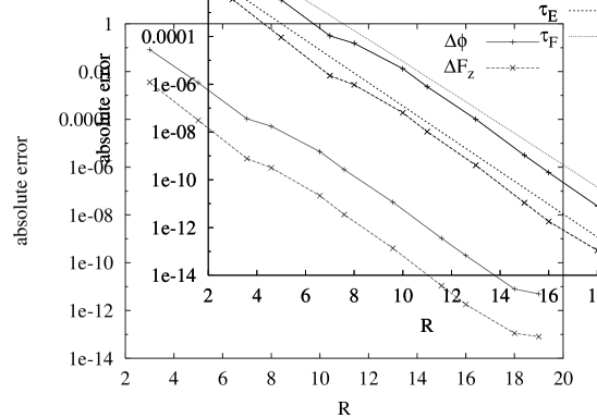
Figure 2: Maximal absolute errors of the $z$–force and the energy for the 2–particle system (compare text)

5.3 Randomly distributed systems

Now we want to investigate the RMS–error scaling of MMM2D and the computation time for larger systems. The systems investigated consist of $N$ particles placed randomly in a cubic simulation box of unit length. Half of the particles carry a charge of $1$, half of them a charge of $-1$. For the calculations MMM2D was tuned to a maximal pairwise error of $\epsilon=10^{-4}$.

The error distribution is highly non–uniform as we have shown before. Therefore it is more safe to use the error formulas given above to constrain the maximal pairwise error rather than the RMS–error, as is done usually. Nevertheless we investigated the actual RMS–error for the uniformly random systems described above. Figure 3 shows the RMS–error for different particle numbers and slice numbers. By the arguments given in Sec. 5.2, the error drops when more slices are used.

Figure 3: RMS–error of the forces calculated by MMM2D for different values of $B$ in dependence of the particle numbers $N$ for fixed $\epsilon=10^{-4}$

If one assumes a standard deviation of the pairwise error of $\sigma$, and furthermore that the pairwise errors are independent, which is true for random systems, it is easy to see that the RMS–error has an expectation value of $\frac{Q^{2}}{\sqrt{N}}\sigma$ [27], with $Q^{2}=\sum_{i}q_{i}^{2}$, which can be seen in Figure 3. Thus our RMS-error behaves like the ones for the usual Ewald methods [27]. Furthermore we have $\sigma\leq\epsilon$ so that the RMS–error can be bounded using our error estimates. Note that again the RMS-error is much smaller than the maximal pairwise error (for 100 particles, $3\cdot 10^{-6}$ instead of $10^{-4}$), although the gain is smaller than for the highly structured systems 1-3.

Having laid the theoretical foundations of the time scaling in Sec. 4, we want to show that the theoretical scaling can be achieved in a real computation. Figure 4 shows the optimal computation time depending on the particle number $N$ for the systems considered above. We also give data for different box heights $\Delta z$. The $x$ and $y$ sides are still fixed to unit length. The pairwise error in the forces was fixed to $\epsilon=10^{-4}$, resulting in the better RMS-errors given above. The optimal number of slices $B$ depends on $\Delta z$. For example, for $\Delta z=0$ we always have $B=1$ and a purely ${\mathcal{O}}(N^{2})$ algorithm, as is seen in the figure. For $\Delta z=1$ the optimal slice numbers were $B=4$ for $N\leq 100$, $B=8$ for $N\leq 1000$ and $B=16$ for $N=4000$, and the ${\mathcal{O}}(N^{5/3})$ scaling is achieved. It can also be seen that MMM2D becomes faster with growing $\Delta z$, as one expects from the error formula. For comparison also computation times for the $2d$–Ewald method (at $\Delta z=1$) and the theoretical scaling curves of ${\mathcal{O}}(N^{5/3})$ and ${\mathcal{O}}(N^{2})$ are included.

The computation times show that MMM2D is always faster than the HBC method, even for small particle numbers (although we achieve a much smaller RMS–error). This can also be seen in the computation times given in Tab.1. These computation times also demonstrate that increasing the precision does not massively impact the computation time of MMM2D. This is due to the exponential error decrease with respect to the cutoff $R$. Since System 1 in this table is purely two dimensional, MMM2D only uses the near formula for the calculation. Therefore even our near formula is superior to the $2d$–Ewald method.

Since MMM2D and the algorithm described by Smith [15] are similar up to the difference that Smith uses the $2d$–Ewald method instead of our near formula, MMM2D is also faster than the algorithm of Smith. From the numbers given by Widmann [10] one can furthermore conclude that MMM2D is also faster than the algorithm proposed by Hautman and Klein[12], although we did not test this method explicitly.

MMM2D is also similar in speed at our accuracy with respect to the two recent Ewald-type algorithms proposed in Refs. [16, 17]. However, these two methods also have the drawback that no error estimates exist, and these will also be hard to develop because of the numerical integration involved. Furthermore it seems unreasonable that their algorithm gets slower for larger $\Delta z$, while MMM2D gets faster, and that their algorithm is fastest for the largest tested real-space cutoffs[16] although they claim that their new Fourier-space expression is responsible for the increase in speed. On the basis of their numbers and non-comparable test cases we are unable to draw further conclusions.

Figure 4: Optimal computation times for different particle numbers $N$.

6 Conclusion

We developed a new method termed MMM2D to accurately calculate the electrostatic energy and forces on charges being distributed in a two dimensional periodic array of finite thickness (2d+h geometry). It has the advantage of requiring only a computational time of ${\mathcal{O}}(N^{5/3})$ instead of a quadratic scaling as previous methods show. It is based on a convergence factor approach and as such does not require any fine–tuning of any Ewald parameters for convergence. Moreover, we derived rigorous error bounds and numerically verified them on specific examples.

Our method is not only asymptotically faster than all $2d$–Ewald methods, but is about four times faster than the HBC method for small numbers of particles, and should also be superior to the method of Hautman and Klein, and to the new methods of Refs. [16, 17] at our accuracies. Our energy and force results achieve a maximal pairwise error of $10^{-4}$ with minimal cutoffs, and $10^{-8}$ can easily be achieved without large increase in computational time. Therefore our method is even more superior whenever a high accuracy is needed. Although the presented formulas may look awkward at the beginning, once implemented, the method is easy to use because the cutoffs for the sums can be easily determined at runtime. Only the number of slices $B$ must be optimized for speed, but, although not implemented, this parameter could also be determined during execution. This is in contrast to basically all $2d$–Ewald methods, for which the tuning of the various parameters is very crucial and error estimates do not exist.

The numerical code for MMM2D in C++ can be requested from the authors. This code also provides interfaces for use with FORTRAN and C.

Appendix A Equivalence of the sum with the convergence factor

Let $p\in\mathbb{R}^{3}$ and for $k,l\in\mathbb{Z}$ let $n_{kl}:=(k\lambda_{x},l\lambda_{y},0)^{T}$ and $n=|n_{kl}|=\sqrt{k^{2}\lambda_{x}^{2}+l^{2}\lambda_{y}^{2}}$. Then it can be shown that for charge neutral systems

$$\frac{1}{|p+n_{kl}|}+\frac{1}{|p-n_{kl}|}-\frac{2}{n}\,=\,{\mathcal{O}}\left(n^{-3}\right)$$ (28)

(see for example [5] or [25]).

Now we rewrite the sum with the convergence factor as

$$\begin{split}&\sum_{S=0}^{\infty}\sum_{k^{2}+l^{2}=S}\sideset{}{{}^{\prime}}{\sum}_{j=1}^{N}\frac{q_{j}e^{-\beta|p_{j}+n_{kl}|}}{|p_{j}+n_{kl}|}\\ &=\,\sum_{k,l\in\mathbb{Z}}\frac{1}{2}\sideset{}{{}^{\prime}}{\sum}_{j=1}^{N}q_{j}\left(\frac{e^{-\beta|p_{j}+n_{kl}|}}{|p_{j}+n_{kl}|}+\frac{e^{-\beta|p_{j}-n_{kl}|}}{|p_{j}-n_{kl}|}-\frac{2e^{-\beta n}}{n}\right)\,\text{.}\end{split}$$ (29)

For any $\alpha_{n}$ where $\beta|\alpha_{n}-n|<1$

$$\frac{e^{-\beta(\alpha_{n}-n)}}{\alpha_{n}}\,=\,\frac{1}{\alpha_{n}}\sum_{l=0}^{\infty}\frac{(-1)^{l}}{l!}\beta^{l}(\alpha_{n}-n)^{l}\,=\,\frac{1}{\alpha_{n}}+\beta\left(\frac{n}{\alpha_{n}}-1\right)+\theta(\beta,\alpha_{n},n)$$ (30)

where $|\theta(\beta,\alpha_{n},n)|\leq\frac{1}{2}\frac{\beta^{2}(\alpha_{n}-n)^{2}}{\alpha_{n}}$.

Therefore for sufficient small $\beta$ we have

$$\begin{split}&\left|\frac{e^{-\beta|p+n_{kl}|}}{|p+n_{kl}|}+\frac{e^{-\beta|p-n_{kl}|}}{|p-n_{kl}|}-\frac{2e^{-\beta n}}{n}\right|\\ &\leq\,e^{-\beta n}\left|\frac{1}{|p+n_{kl}|}+\frac{1}{|p-n_{kl}|}-\frac{2}{n}\right|\\ &\quad+e^{-\beta n}\beta\left|\left(\frac{n}{|p+n_{kl}|}-1\right)+\left(\frac{n}{|p-n_{kl}|}-1\right)\right|\\ &\quad+e^{-\beta n}\left|\theta(\beta,|p+n_{kl}|,n)+\theta(\beta,|p-n_{kl}|,n)\right|\\ &=\,\frac{e^{-\beta n}}{n^{3}}{\mathcal{O}}(1)+\frac{\beta e^{-\beta n}}{n^{2}}{\mathcal{O}}(1)+\frac{\beta^{2}e^{-\beta n}}{n}{\mathcal{O}}(1)\,\text{.}\end{split}$$

This can be seen by applying equation (28) to the two first terms and equation (30) to the last. By approximating the sums over these terms separately as integrals it is easy to see that the sum in equation (29) converges uniformly for small $\beta$ and therefore

$$\begin{split}&\lim_{\beta\rightarrow 0}\sum_{k,l\in\mathbb{Z}}\frac{1}{2}\sideset{}{{}^{\prime}}{\sum}_{j=1}^{N}q_{j}\left(\frac{e^{-\beta|p_{j}+n_{kl}|}}{|p_{j}+n_{kl}|}+\frac{e^{-\beta|p_{j}-n_{kl}|}}{|p_{j}-n_{kl}|}-\frac{2e^{-\beta n}}{n}\right)\\ &=\sum_{k,l\in\mathbb{Z}}\frac{1}{2}\sideset{}{{}^{\prime}}{\sum}_{j=1}^{N}q_{j}\left(\frac{1}{|p_{j}+n_{kl}|}+\frac{1}{|p_{j}-n_{kl}|}-\frac{2}{n}\right)\\ &=\sum_{S=0}^{\infty}\sum_{k^{2}+l^{2}=S}\sideset{}{{}^{\prime}}{\sum}_{j=1}^{N}\frac{q_{j}}{|p_{j}+n_{kl}|}\,\text{.}\end{split}$$ (31)

References

• [1] P.Β Ewald, Die Berechnung optischer und elektrostatischer Gitterpotentiale, Ann. Phys. 64 (1921) 253–287.
• [2] J.Β Kolafa, J.Β W. Perram, Cutoff errors in the ewald summation formulae for point charge systems, Molecular Simulation 9Β (5) (1992) 351–68.
• [3] R.Β Sperb, An alternative to ewald sums - part i: Identities for sums, Molecular Simulation 20Β (3) (1998) 179–200.
• [4] S.Β W. deΒ Leeuw, J.Β W. Perram, E.Β R. Smith, Simulation of electrostatic systems in periodic boundary conditions. i. lattice sums and dielectric constants, Proc. R. Soc. Lond. A 373 (1980) 27–56.
• [5] S.Β W. deΒ Leeuw, J.Β W. Perram, E.Β R. Smith, Simulation of electrostatic systems in periodic boundary conditions. ii. equivalence of boundary conditions, Proc. R. Soc. Lond. A 373 (1980) 57–66.
• [6] R.Β Sperb, R.Β Strebel, An alternative to ewald sums, part 3: Implementation and results, Molecular Simulation 27Β (1) (2001) 61–74.
• [7] R.Β W. Hockney, J.Β W. Eastwood, Computer Simulation Using Particles, IOP, London, 1988.
• [8] M.Β Deserno, C.Β Holm, How to mesh up Ewald sums. i. a theoretical and numerical comparison of various particle mesh routines, J. Chem. Phys. 109 (1998) 7678.
• [9] J.Β Lekner, Summation of coulomb fields in computer simulated disordered systems, Physica A 176 (1991) 485–498.
• [10] A.Β H. Widmann, D.Β B. Adolf, A comparison of ewald summation techniques for planar surfaces, Comp. Phys. Comm. 107 (1997) 167–186.
• [11] D.Β M. Heyes, M.Β Barber, J.Β H.Β R. Clarke, Molecular dynamics computer simulation of surface properties of crystalline potassium chloride, J. Chem. Soc. Faraday Trans. II 73 (1977) 1485.
• [12] J.Β Hautman, M.Β L. Klein, An ewald summation method for planar surfaces and interfaces, Mol. Phys. 75 (1992) 379.
• [13] B.Β R.Β A. Nijboer, F.Β W. deΒ Wette, On the calculation of lattice sums, Physica 23 (1957) 309–321.
• [14] B.Β Nijboer, On the electrostatic potential due to a slab shaped and a semi-infinite nacl-type lattice, Physica A 125 (1984) 275–279.
• [15] E.Β R. Smith, Electrostatic potentials for thin layers, Mol. Phys. 65 (1988) 1089–1104.
• [16] M.Β Kawata, M.Β Mikami, Rapid calculation of two-dimensional ewald summation, Chem. Phys. Lett. 340 (2001) 157–164.
• [17] M.Β Kawata, U.Β Nagashima, Particle mesh ewald method for three-dimensional systems with two-dimensional periodicity, Chem. Phys. Lett. 340 (2001) 165–172.
• [18] A.Β Arnold, C.Β Holm, Chem. Phys. Lett. to appear.
• [19] J.Β Lekner, Physica A 157 (1989) 826.
• [20] R.Β Sperb, Extension and simple proof of lekner’s summation formula for coulomb forces, Molecular Simulation 13 (1994) 189–193.
• [21] F.Β S. Csajka, C.Β Seidel, Strongly charged polyelectrolyte brushes: A molecular dynamics study, Macromolecules 33 (2000) 2728–2739.
• [22] R.Β Strebel, Pieces of software for the Coulombic $m$ body problem, Dissertation 13504, ETH Zuerich (1999).
URL http://e-collection.ethbib.ethz.ch/show?type=diss&nr=13504
• [23] F.Β Oberhettinger, Fouriertransforms of distributions and their inverses, Vol.Β 16 of Probability and Mathematical Statistics, Academic Press, New York, 1973.
• [24] M.Β Abramowitz, I.Β Stegun, Handbook of mathematical functions, Dover Publications Inc., New York, 1970.
• [25] A.Β Arnold, Berechnung der elektrostatischen wechselwirkung in 2d + h periodischen systemen, Diploma thesis, Johannes Gutenberg-UniversitΓ€t (may 2001).URL
http://www.mpip-mainz.mpg.de/www/theory/phd_work/dipl-arnold.ps.gz
• [26] GNU, Gnu scientific library (GSL) .
URL ftp://sources.redhat.com/pub/gsl
• [27] M.Β Deserno, C.Β Holm, How to mesh up Ewald sums. ii. an accurate error estimate for the p3m algorithm, J. Chem. Phys. 109 (1998) 7694.