Green’s function approach to the magnetic properties of the kagomé antiferromagnet

Abstract

The $S=1/2$ Heisenberg antiferromagnet is studied on the kagomé lattice by using a Green’s function method based on an appropriate decoupling of the equations of motion. Thermodynamic properties as well as spin-spin correlation functions are obtained and characterize this system as a two-dimensional quantum spin liquid. Spin-spin correlation functions decay exponentially with distance down to low temperature and the calculated missing entropy at $T=0$ is found to be $0.46\ln{2}$. Within the present scheme, the specific heat exhibits a single peak structure and a $T^{2}$ dependence at low temperature.

I Introduction

Antiferromagnetic spin systems on fully frustrated lattices show many unusual behaviors in magnetic and thermal propertiesLiebmann ; Ramirez . One of the main ingredients is that their unit cell allows for a continuous degree of freedom and that the connectivity (corner sharing) allows for an extensive number of these degrees of freedom in the classical ground state. More subtle phenomena appear when looking at quantum models on these lattices as quantum fluctuations may induce very unsusual ground states. In particular, wether the quantum ground state on fully frustrated lattices may not break the lattice symmetry nor the spin group symmetry is still a highly debated question. A lot of work has been done to answer this question in the framework of the proposition of Andersonanderson , looking first at Resonating Valence Bond states.

One of the most studied candidates is the quantum $S$=1/2 Heisenberg antiferromagnet on the kagomé lattice. Using various methodse89 ; ze95 ; ce92 ; le93 ; lblps97 ; web98 ; ey94 ; mila98 ; si00 , it has been shown that the low temperature physics should be dominated by short range RVB states which produce a continuum of singlet states between the $S=0$ ground state and the first excited $S=1$ state. A still controversial question is the presence of a very low temperature peak in the specific heat, much below the one corresponding to the onset of short range correlations, that could be ascribed to a high density of singlet states in the singlet-triplet spin gap. Associated to this low temperature peak is the missing (or not) entropy that would characterize an ordered or a disordered ground state.

The experimental relevance of the model is extremely fragile as, in real compounds, many other parameters may drive the physics to very different universality classes, described through inclusion of next nearest neighbor interactionsrei91 , disordershender93 , antisymmetric interactionselhajal01 , etc… Nevertheless, in many cases, the Heisenberg antiferromagnet is a good starting point as it is generally believed that many properties of realistic systems come from deviations from the Heisenberg limit. Examples are the layered oxide SrCr_9pGa_12-9pO₁₉rec90 ; ukkll94 ; lbar96 ($S=3/2$) or the organic pseudo-$S=1$ compound m-MPYNN.BF₄wkyoya97 .

In this paper, the properties of the Heisenberg $S$=1/2 kagomé antiferromagnet are addressed by using a spin Green’s functions technique. One of the advantages of the method is that it is well suited for magnetic systems with no long range order as it uses a decoupling scheme based on short ranged spin correlations. This method was previously introduced by Kondo and Yamagiky72 in the context of the one-dimensional Heisenberg model as a theory of spin-waves in absence of long-range order. More recently, it has been used to address different problemssh91 ; yf00 and can be extended to include magnetic phasesgp02 . Here, the formalism is used to compute thermodynamic and magnetic quantities at all temperatures, like the internal energy, specific heat, entropy, magnetic susceptibility and structure factor. Correlation functions are also computed at all temperatures and for various separation distances. In the next section, the approximation is presented and results are discussed in Sec. III.

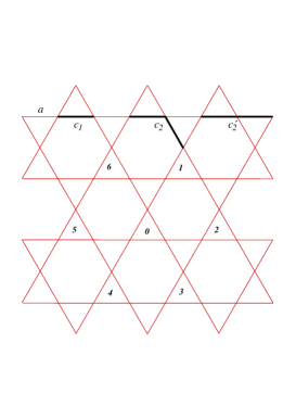
Figure 1: The kagomé lattice.

II Model and Approximation

The antiferromagnetic Heisenberg model is defined by the Hamiltonian

$${\cal H}=\frac{1}{2}\sum_{ij}J_{ij}\ {\bf S}_{i}\cdot{\bf S}_{j}.$$ (1)

where we assume $S=1/2$ and a nearest-neighbor exchange

$$J_{ij}=\begin{cases}J(>0)&\text{if $i,j$ are nearest neighbors}\\ 0&\text{otherwise.}\end{cases}$$ (2)

The spin susceptibility

$$\chi_{ij}(\omega)\equiv\ll S^{-}_{i};S^{+}_{j}\gg_{\omega}$$ (3)

is obtained by a Fourier transformed Green’s function

$$\ll A;B\gg_{\omega}=\int\ll A;B\gg_{t}e^{i\omega t}dt$$ (4)

where

$$\ll A;B\gg_{t}\equiv-i\theta(t)\left<\left[\hat{A}(t),\hat{B}(0)\right]\right>.$$ (5)

¿From the equation of motion of the operator $\hat{A}(t)$ in the Heisenberg representation, the Green’s functions above must satisfy the equation

$$\omega\ll A;B\gg_{\omega}=\left<\left[A,B\right]\right>+\ll\left[A,{\cal H}\right];B\gg_{\omega}.$$ (6)

The spin susceptibility of the present model can be obtained by

$$\omega\chi_{ij}(\omega)=-2\delta_{ij}\left<S^{z}_{i}\right>+\sum_{k}J_{ik}\left(\Gamma_{kij}(\omega)-\Gamma_{ikj}(\omega)\right).$$ (7)

The three operator Green’s functions

$$\Gamma_{ikj}(\omega)\equiv\ll S^{z}_{i}S^{-}_{k};S^{+}_{j}\gg_{\omega}$$ (8)

must also obey their corresponding equations

$$\omega\Gamma_{ikj}(\omega)=\left(\delta_{ij}-\delta_{kj}\right)\left<S^{+}_{i}S^{-}_{k}\right>_{\omega}\\ +1/2\sum_{l}J_{il}\ll\left(S^{+}_{i}S^{-}_{l}-S^{-}_{i}S^{+}_{l}\right)S^{-}_{k};S^{+}_{j}\gg_{\omega}\\ +\sum_{l}J_{kl}\ll S^{z}_{i}\left(S^{z}_{l}S^{-}_{k}-S^{z}_{k}S^{-}_{l}\right);S^{+}_{j}\gg,$$ (9)

As higher-order Green’s functions are generated, one obtains an infinite hierarchy of equations which have to be decoupled in order to obtain $\chi_{ij}(\omega)$.

In a frustrated lattice, one is constrained to the non-magnetic phase, where $\left<S_{i}^{z}\right>=\left<S_{i}^{\pm}\right>=0$ and $\left<S_{i}^{+}S_{j}^{-}\right>=2\left<S_{i}^{z}S_{j}^{z}\right>$.

Here we adopt an extension of the Kondo-Yamaji decoupling approximation for the kagomé lattice, assuming (only for different sites $i,l,k$)

$$\ll S_{i}^{-}S_{l}^{+}S_{k}^{-};S_{j}^{+}\gg_{\omega} \approx \alpha\left<S_{i}^{-}S_{l}^{+}\right>\chi_{kj}(\omega)$$ (10)

$$+\alpha\left<S_{l}^{+}S_{k}^{-}\right>\chi_{ij}(\omega),$$

$$\ll S_{i}^{z}S_{l}^{z}S_{k}^{-};S_{j}^{+}\gg_{\omega} \approx \alpha\left<S_{i}^{z}S_{l}^{z}\right>\chi_{kj}(\omega).$$ (11)

The static correlation functions $\left<S_{i}^{+}S_{j}^{-}\right>$ between spins at the lattice positions ${\bf R}_{i}$ and ${\bf R}_{j}$ depend on the distance $d=|{\bf R}_{i}-{\bf R}_{j}|$, on the number $n$ of bonds between sites $i$ and $j$, and on the lattice symmetry. As a shorthand notation, we shall call the local correlation as $c_{0}=\left<S^{+}_{i}S^{-}_{i}\right>$, the nearest-neighbor correlation as $c_{1}$ and the next-nearest-neighbor correlations as $c_{2}$ and $c_{2}^{\prime}$ (the former corresponding to the shortest distance, as illustrated in figure 1). We also introduce $\tilde{c}_{n}^{(\prime)}=\alpha c_{n}^{(\prime)}$. The parameter $\alpha$ is useful to enforce the condition $c_{0}=1/2$ ky72 .

These correlation functions can be evaluated from the spin susceptibility as

$$\left<S^{+}_{j}S^{-}_{i}\right>=-\frac{1}{\pi}\ \int\frac{{\rm Im}\chi_{ij}(\omega+i\eta)}{1-e^{-\beta\omega}}\ d\omega.$$ (12)

Thus, $c_{1}$, $c_{2}$, and $c_{2}^{\prime}$ and also the parameter $\alpha$ appearing in Eqs. 10-11 must be evaluated selfconsistently.

Applying approximation 10-11 to the kagomé lattice yields

$$\left[\omega^{2}-4J^{2}\tilde{c}\right]\chi_{ij}(\omega)=-8Jc_{1}\delta_{ij}+2c_{1}J_{ij}\\ +J\tilde{c}_{1}\sum_{k}J_{ik}^{\prime}\chi_{kj}(\omega)-J\left(\tilde{c}+2\tilde{c}_{1}\right)\sum_{k}J_{ik}\chi_{kj}(\omega),$$ (13)

where

$$\tilde{c}=1/2+\tilde{c}_{1}+\tilde{c}_{2}+\tilde{c}_{2}^{\prime}$$ (14)

and

$$J_{ij}^{\prime}=\begin{cases}J&\text{if i, j are next-nearest neighbors,}\\ 0&\text{otherwise.}\end{cases}$$ (15)

By working directly with the $\tilde{c}_{n}^{(\prime)}$, the numerical problem is reduced to only two selfconsistent parameters, $\tilde{c}_{1}$ and $\tilde{c}_{2}+\tilde{c}_{2}^{\prime}$, from which one can obtain $\alpha=2\tilde{c}_{0}$.

With reference to the underlying triangular lattice, the approximate equation 13 can be rewritten in matrix form

$$\left[\omega^{2}-4J^{2}\tilde{c}\right]\boldsymbol{\chi}_{ij}(\omega)=-2c_{1}\left(4J\delta_{ij}\boldsymbol{\mathit{1}}-\boldsymbol{J}_{ij}\right)\\ +J\tilde{c}_{1}\sum_{k}\boldsymbol{J}_{ik}^{\prime}\boldsymbol{\chi}_{kj}(\omega)-J\left(\tilde{c}+2\tilde{c}_{1}\right)\sum_{k}\boldsymbol{J}_{ik}\boldsymbol{\chi}_{kj}(\omega)\ ,$$ (16)

where $\boldsymbol{J}_{ij}$ and $\boldsymbol{J}^{\prime}_{ij}$ are the exchange matrices connecting neighboring triangles. As indicated in Fig. 1, each triangle is surrounded by six neighboring triangles, all of them contributing to both types of exchange matrices.

The elements of the dynamic susceptibility matrix are defined as

$$\chi^{ab}({\bf q},\omega)=\frac{1}{N}\sum_{i,j}\chi^{ab}_{ij}(\omega)\ e^{-i{\bf q}\cdot({\bf R}_{i}^{a}-{\bf R}_{j}^{b})}$$ (17)

where ${\bf R}_{i}^{a}={\bf R}_{i}+{\bf T}_{a}$, ${\bf R}_{i}$ is the lattice position of the $i$-th triangle, and the vectors ${\bf T}_{a}$ indicate the position of site $a$ in the triangular unit cell ($a=1,2,3$).

Applying a corresponding Fourier transformation to equation 16 gives

$$\boldsymbol{\chi}({\bf q},\omega)=-2c_{1}\boldsymbol{A}^{-1}({\bf q},\omega)\ \boldsymbol{B}({\bf q})$$ (18)

where

$$\boldsymbol{A}({\bf q},\omega) = \left(\omega^{2}-4J^{2}\tilde{c}\right)\boldsymbol{\mathit{1}}-J\tilde{c}_{1}\boldsymbol{J}^{\prime}({\bf q})$$ (19)

$$+J\left(\tilde{c}+2\tilde{c}_{1}\right)\boldsymbol{J}({\bf q}),$$

$$\boldsymbol{B}({\bf q}) = 4J\boldsymbol{\mathit{1}}-\boldsymbol{J}({\bf q}),$$ (20)

where $\boldsymbol{J}({\bf q})$ and $\boldsymbol{J}^{\prime}({\bf q})$ are the Fourier transform of the exchange matrices $\boldsymbol{J}_{ij}$ and $\boldsymbol{J}^{\prime}_{ij}$,

$$\boldsymbol{J}({\bf q})=2J\left(\begin{array}[]{ccc}0&{\rm cos}[(x-\sqrt{3}y)/4]&{\rm cos}[(x+\sqrt{3}y)/4]\\ \\ {\rm cos}[(x-\sqrt{3}y)/4]&0&{\rm cos}(x/2)\\ \\ {\rm cos}[(x+\sqrt{3}y)/4]&{\rm cos}(x/2)&0\\ \end{array}\right)\ ,$$ (21)

$$\boldsymbol{J}^{\prime}({\bf q})=2J\left(\begin{array}[]{ccc}2{\rm cos}(x/2){\rm cos}(\sqrt{3}y/2)&{\rm cos}[(3x+\sqrt{3}y)/4]&{\rm cos}[(3x-\sqrt{3}y)/4]\\ \\ {\rm cos}[(3x+\sqrt{3}y)/4]&{\rm cos}x+{\rm cos}[(x-\sqrt{3}y)/2]&{\rm cos}(\sqrt{3}y/2)\\ \\ {\rm cos}[(3x-\sqrt{3}y)/4]&{\rm cos}(\sqrt{3}y/2)&{\rm cos}x+{\rm cos}[(x+\sqrt{3}y)/2]\\ \end{array}\right)\ .$$ (22)

in which $x=q_{x}a$ and $y=q_{y}a$.

It follows that

$$\boldsymbol{\chi}({\bf q},\omega)=-2c_{1}\frac{\boldsymbol{P}({\bf q},\omega^{2})}{\Delta({\bf q},\omega^{2})}$$ (23)

where $\Delta({\bf q},\xi)$ is a third degree polynomial in $\xi$ with ${\bf q}$-dependent coefficients and the elements of $\boldsymbol{P}({\bf q},\xi)$ are second degree polynomials in $\xi$ with ${\bf q}$-dependent coeficients. The dynamic susceptibility can be finally writen as

$$\boldsymbol{\chi}({\bf q},\omega)=-2c_{1}\sum_{l=1}^{3}\frac{\boldsymbol{R}_{l}({\bf q})}{\omega^{2}-\Omega_{l}^{2}({\bf q})}$$ (24)

where

$$\boldsymbol{R}_{l}({\bf q})=\frac{\boldsymbol{P}({\bf q},\Omega_{l}^{2})}{\Delta^{\prime}({\bf q},\Omega_{l}^{2})}$$ (25)

and

$${\Delta^{\prime}({\bf q},\xi)}=\frac{\partial}{\partial\xi}\Delta({\bf q},\xi)\ .$$ (26)

The $\Omega_{l}({\bf q})$ are excitation energies, obtained from the roots $\xi_{l}=\Omega_{l}^{2}({\bf q})$ of the polynomial $\Delta({\bf q},\xi)$. One of these roots, $\Omega_{1}^{2}({\bf q})=6J^{2}(\tilde{c}+\tilde{c_{1}})$, is found to be non-dispersive over the whole Brillouin zone. Thus, the dispersion in the energy spectrum is due to the other roots ($l=2,3$), which are evaluated numerically.

By writing the correlation functions of eq. 12 in matrix form and performing the inverse Fourier transformation, we can show that

$$c_{ij}^{ab}=-2c_{1}\sum_{l=1}^{3}\sum_{\bf q}b_{l}({\bf q})\ R_{l}^{ab}({\bf q})\ {\rm cos}\{{\bf q}\cdot({\bf R}_{i}^{a}-{\bf R}_{j}^{b})\}$$ (27)

where

$$b_{l}({\bf q})=\frac{n(\Omega_{l})-n(-\Omega_{l})}{2\Omega_{l}},$$ (28)

and $n(\omega)$ is the Bose distribution function. The sum over momenta must be performed numerically.

The dynamic structure factor matrix is related to the dynamic susceptibility by

$$\boldsymbol{S}({\bf q},\omega)=-\frac{2{\rm Im}\ \boldsymbol{\chi}({\bf q},\omega)}{1-e^{-\beta\omega}}.$$ (29)

After obtaining the selfconsistent parameters, the static structure factor can be evaluated by

$$\boldsymbol{S}({\bf q})=2c_{1}\sum_{l=1}^{3}\sum_{\bf q}b_{l}({\bf q})\ \boldsymbol{R}_{l}({\bf q}).$$ (30)

III Results

We have calculated the selfconsistent values of $c_{1}$, $c_{2}$, and $c_{2}^{\prime}$ as a function of temperature. They are plotted in fig. 2-b. The selfconsistent parameter $\alpha$ is shown in fig. 2-a. From the knowledge of these selfconsistent functions all missing correlation functions can be evaluated. In figure 3 we show the correlation functions $c_{n}^{(\prime)}$ between sites separated by at most 6 lattice bonds. The distribution of the points is very similar to that obtained in Ref. cl98, for the pyrochlore lattice, indicating an exponential decay with a correlation length of the order of the lattice parameter $a$.

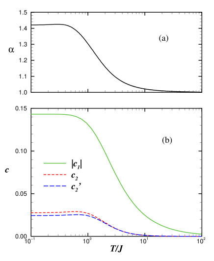
Figure 2: (a) The selfconsistent parameter $\alpha$ and (b) the correlation functions $c_{1}$, $c_{2}$ and $c_{2}^{\prime}$ as a function of temperature.

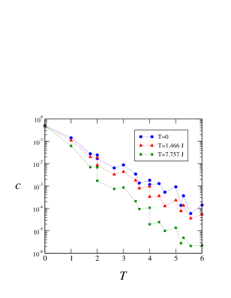
Figure 3: Correlation functions versus distance (in units of the lattice parameter $a$).

The internal energy is given by $E=-6NJc_{1}$. The ground-state value $E=-0.859NJ$ is in good agreement with earlier calculations (see Refs. lblps97, ; yf00, ; ch90, ). In figure 4 we present the specific heat $C=dE/dT$. This curve has a single peak and is very similar to the result of high-temperature expansions ey94 reproducing the high-temperature limit $C\sim T^{-2}$. In the low-temperature limit, the time involved in the numerical computation increases with decreasing temperature, because the convergence of the integral in ${\bf q}$ becomes slower, and in addition one needs a higher precision in order to perform the derivative involved in the evaluation of the specific heat. Nevertheless, a careful analysis of the numerical results indicates unambiguously a $T^{2}$ dependence of the specific heat which extends to very low temperatures. Therefore, there will be no second peak in the present model. The fact that the specific heat does not vanish exponentially indicates the presence of low energy states even though the low-temperature peak found in Ref. si00, is missing. Indeed, it should be emphasized that it is not sure that this peak will persist in the thermodynamic limitsin01 which supports the results obtained in the present work. The change in entropy $\int_{0}^{T}\frac{C(T^{\prime})}{T^{\prime}}dT^{\prime}$ is also shown in Fig. 4. The total change in entropy is $0.54\ln{2}$, corresponding to a ground-state entropy $0.46\ln{2}$, of the same order as found in Ref. ey94, .

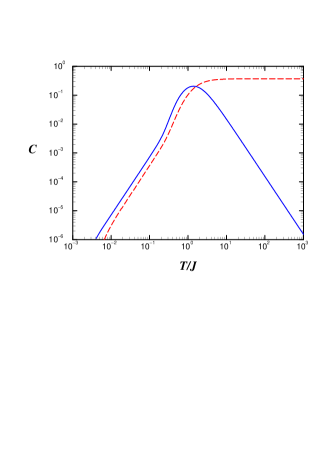
Figure 4: Specific heat as a function of temperature (solid line). The dashed line gives the integrated entropy.

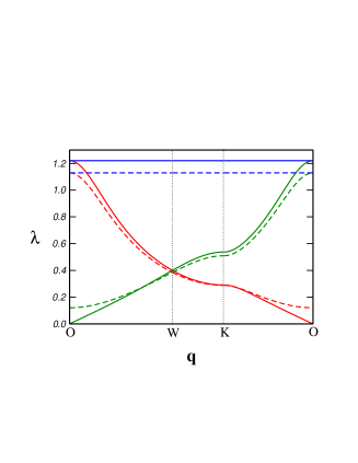
Figure 5: The eigenvalues $\lambda_{n}({\bf q})$ of the structure factor along some symmetry directions in ${\bf q}$-space at $T=0$ (solid lines) and for an intermediate value of $T$ (dashed lines).

The eigenvalues $\lambda_{n}({\bf q})$ of the structure factor are shown in Fig. 5. The result is remarkably similar to what is found from the high-temperature expansions of Ref. ey94 . Whithin the present approach one can easily follow the effect of temperature on the structure factor for all wavevectors even at very low $T$. We observe that its highest eigenvalue is degenerate over the whole Brillouin zone. For the pyroclore, the structure factor is a $4\times 4$ matrix, which has one additional eigenvalue. In a perturbative expansion cl98 the two highest eigenvalues are found to lie very close to each other, one of them being completely degenerate while the other one has a weakly lifted degeneracy, which is crucial to reproduce the main features of neutron scattering experiments. As a further work, it would be interesting to extend the present approach to the pyrochlore antiferromagnet.

- (1) R. Liebmann: Statistical Mechanics of Periodic Frustrated Ising Systems, (Springer, Berlin, 1986).
- (2) A. P. Ramirez, Ann. Rev. Mater. Sci 24, 453 (1994), P. Schiffer and A. P. Ramirez, Comments Condens. Matter Phys. 18, 21 (1996) and references therein.
- (3) P. W. Anderson, B. Halperin and C. M. Varma, Phisos. Mag. 25, 1 (1972).
- (4) V. Elser, Phys. Rev. Lett. 62, 2405 (1989).
- (5) C. Zeng and V. Elser, Phys. Rev. B 51, 8318 (1995).
- (6) J. Chalker and J. Eastmond, Phys. Rev. B 46, 14201 (1992).
- (7) P. Leung and V. Elser, Phys. Rev. B 47, 5459 (1993).
- (8) P. Lecheminant et al., Phys. Rev. B 56, 2521 (1997).
- (9) C. Waldtmann et al., Eur. Phys. J. B 2, 501 (1998).
- (10) N. Elstner and A. P. Young, Phys. Rev. B 50, 6871 (1994).
- (11) F. Mila, Phys. Rev. Lett. 81, 2356 (1998).
- (12) P. Sindzingre, G. Misguich, C. Lhuillier, B. Bernu, L. Pierre, Ch. Waldtmann, and H.-U. Everts, Phys. Rev. Lett. 84, 2953 (2000).
- (13) J. N. Reimers, A. J. Berlinsky and A.-C. Shi., Phys. Rev. B 43 (1991) 865.
- (14) E. F. Shender, V. B. Cherepanov, P. C. W. Holdsworth, and A. J. Berlinsky, Phys. Rev. Lett. 70, 3812-3815 (1993).
- (15) M. Elhajal, B. Canals, C. Lacroix, to be published.
- (16) A. Ramirez et al., Phys. Rev. Lett. 64, 2070 (1992).
- (17) Y. Uemura et al., Phys. Rev. Lett. 73, 3306 (1994).
- (18) S.-H. Lee et al., Europhys. Lett 35, 127 (1996).
- (19) N. Wada et al., J. Phys. Soc. Jpn. 66, 961 (1997).
- (20) J. Kondo and K. Yamaji, Prog. Theor. Phys. 47, 807 (1972).
- (21) H. Shimahara, S. Takada, J. Phys. Soc. Jap. 60, 2394 (1991).
- (22) W. Yu and S. Feng, Eur. Phys. J. B 13, 265 (2000).
- (23) M. E. Gouvêa and A. S. T. Pires, to be published
- (24) B. Canals and C. Lacroix, Phys. Rev. Lett. 80, 2933 (1998).
- (25) Chen Zeng and Veit Elser, Phys. Rev. B 42, 8436 (1990).
- (26) P. Sindzingre, private communication.