Completely monotone solutions of the mode-coupling theory for mixtures

Abstract

We establish that a mode-coupling approximation for the dynamics of multi-component systems obeying Smoluchowski dynamics preserves a subtle yet fundamental property: the matrices of partial density correlation functions are completely monotone, i.e. they can exactly be written as superpositions of decaying exponentials only. This statement holds, no matter what further approximations are needed to calculate the theory’s coupling parameters. The long-time limit of these functions fulfills a maximum property, and an iteration scheme for its numerical determination is given. We also show the existence of a unique solution to the equations of motion for which power series both for short times and small frequencies exist, the latter except at special points where ergodic-to-nonergodic transitions occur. These transitions are bifurcations that are proven to be of the cuspoid family.

I Introduction

Density correlation functions are convenient tools to characterize the dynamics of liquids or disordered systems. They can be measured in experiment, e.g. by inelastic neutron scattering, dynamic light scattering in colloidal systems, or can be determined from computer simluation techniques. On the other hand, one can calculate them from theory, but in the case of strongly interacting systems, one typically has to invoke certain approximations in order to obtain the desired results. There are, however, some general properties of such correlation functions, directly related to the time-evolution operator of the system. It is a nontrivial point to show that all approximations involved in deriving a theory’s equations of motion preserve these general properties.

One example are colloidal suspensions obeying Smoluchowski dynamics. One knows from general grounds that in such systems the matrices of partial correlation functions are completely monotone, i.e. they can be written as a superposition of decaying exponentials only. An approximative theory calculating such quantities should aim to reproduce these properties, since they are direct consequences of the structure of the time-evolution operator. However, the concept of complete monotonicity is quite subtle, and it is therefore likely that a given approximation prevents the approximative solutions from sharing this feature with the complete solution.

At high densities, colloidal systems are known to undergo glassy dynamics, provided crystallization can be suppressed for a sufficiently long time. In these cases the so-called mode-coupling theory of the glass transition (MCT) has been successful in describing much of the experimental facts. For one-component, i.e. monodisperse, systems the theory has been proven Götze and Sjögren (1995) to give results for the density correlation functions, which indeed reproduce the above mentioned features. However, little is known about multi-component, or polydisperse, mixtures. Recently, glassy dynamics in a binary colloidal suspension has been studied Williams and van Megen (2001), challenging detailed comparisons of the MCT for mixtures with experiment.

MCT tries to describe the motion of particles on a microscopic scale by an approximation of the frequency- and wavenumber-dependent viscosity in terms of density-fluctuation products. Such an approach comes about naturally if one considers the potential stresses to be built up by the density fluctuations of the liquid itself. The resulting equations contain a feedback mechanism induced by the slowing down of relaxations due to the so-called cage effect. It has been shown that these equations allow for an ideal glass state, given the interactions are strong enough, e.g. at high densities. The ideal glass is characterized by a nonvanishing long-time limit of density correlation functions which corresponds to an elastic scattering contribution in the dynamical structure factor. In the “phase diagram”, there occur critical manifolds, referred to as glass-transition singularities, that separate ergodic liquid from ideal glass states and can also extend into the glass state. Upon approaching a singularity point, the long-time limit of the density correlators, sometimes referred to as the glass form factor or the Edwards-Anderson parameter of the system, changes discontinuously. This holds for both liquid-glass transitions, where the change is from zero to some nonzero value, as well as glass-glass transitions.

Close to the transition, analytic formulas providing asymptotic solutions of the MCT equations of motion have been derived. There occur two time fractals with nontrivial exponents, and two diverging time scales, accompanied by corresponding scaling laws. On these time scales the dynamics of the glass former is also referred to as structural relaxation. The asymptotic predictions as well as numerical solutions of the full MCT equations for model systems have been extensively tested against experimental data; for a detailed discussion of the glass-transition scenario, the reader is referred to a recent review Götze (1999).

The aim of this paper is to generalize from the case of one-component systems to that of multi-component mixtures proofs of the basic properties of MCT solutions. In particular, we show that the structural relaxation can be represented as a continuous superposition of decaying exponentials, i.e. that the density correlation functions indeed are completely monotone. Furthermore, the long-time limits can be obtained by a simple iteration procedure that does not involve the solution of the complete dynamical equations. An investigation of this iteration brings out glass transitions in general to be bifurcations of the cuspoid type. In addition, a short-time expansion of the density correlation functions is demonstrated to be convergent for short times, and similarly, a power series for small frequencies is shown to exist.

The paper is organized as follows: In Sec. II, we will introduce the equations of motion for the mixtures considered, together with some basic properties and the MCT approximation. Section III presents a proof that the MCT equations of motion have a uniquely determined solution which is completely monotone. In Sec. IV, the long-time limit of these solutions will be discussed, and in Sec. V, the existence of power series solutions both in the time and frequency domain is shown, the latter by proving first that all moments of the correlation functions are finite. Section VI offers some conclusions.

II Equations of Motion

II.1 General Properties

We consider a classical system enlcosed in a box of volume $V$ with a total number of particles $N=\sum_{\nu=1}^{s}N_{\nu}$, consisting of $s$ different species with number concentrations $x_{\nu}=N_{\nu}/N$. The particles are supposed to be structureless, i.e. they do not possess any internal degrees of freedom, and are thus fully described by their positions, momenta, and species index. The variables

$$n_{\nu}(\vec{q})=N^{-1/2}\sum_{i=1}^{N_{\nu}}\exp(i\vec{q}\cdot\vec{r}_{i}^{\nu})$$ (1)

are then the fluctuating densities of species $\nu$ to wave vector $\vec{q}$. Here, $\vec{r}_{i}^{\nu}$ denotes the position of the $i$-th particle of species $\nu$. The simplest statistical information on structural dynamics that can be extracted from a multi-component supercooled liquid is the matrix of density correlation functions

$$\Phi_{\mu\nu}(q,t)=\left\langle n_{\mu}(\vec{q},t)|n_{\nu}(\vec{q})\right\rangle\,.$$ (2)

Here, the brackets $\langle\cdot|\cdot\rangle$ denote the Kubo product with $\langle A|B\rangle=\langle\delta A^{*}\delta B\rangle$, where $\delta A=A-\langle A\rangle$, and $\langle\dots\rangle$ indicates canonical averaging. Since $\Phi_{\mu\nu}(q,t)$ is the spatial Fourier transform of a function that is real, translational-invariant and isotropic, it is itself real and depends only on the magnitude of the wave vector $q=|\vec{q}|$. The time evolution is given by $n_{\mu}(\vec{q},t)=\exp[i{\mathcal{S}}t]n_{\mu}(\vec{q})$. For a liquid obeying Newtonian dynamics, the operator $\mathcal{S}$ is just the Liouville operator, which is Hermitian with respect to the Kubo product. In this case, time inversion symmetry implies the density correlation matrix to be symmetric with respect to interchange of the species indices.

Let us focus on colloidal liquids, and $\mathcal{S}$ denote the Smoluchowski operator. There, time inversion symmetry is broken explicitly, but still the symmetry $\Phi_{\mu\nu}(q,t)=\Phi_{\nu\mu}(q,t)$ holds, although this has to be proven seperately Nägele (1996).

One then has the spectral decomposition $\exp[i{\mathcal{S}}t]=\int\exp(-\gamma t)dP_{\gamma}$, with eigenvalues $\gamma$ fulfilling $\gamma\geq 0$, and $P_{\gamma}$ denoting the projector onto the corresponding linear subspace. This immediately leads to the following representation:

$$\Phi_{\mu\nu}(q,t)=\int e^{-\gamma t}da_{\mu\nu,q}(\gamma)\,,$$ (3)

where the measure $a$ is concentrated on the nonnegative real axis, is symmetric in $\mu,\nu$, and positve: $da_{\mu\nu,q}(\gamma)\succeq 0$, i.e. for any set of complex numbers $y_{\nu}$, $\nu=1,\dots,n$, the measure $y_{\mu}^{*}\,da_{\mu\nu,q}(\gamma)\,y_{\nu}$ is positive (summation over repeated indices is implied here and in the following). A function having these properties is called completely monotone. In particular, $\Phi_{\mu\nu}(q,t)$ is a positive definite matrix for all times, and for all $l$ the time derivatives $(-1)^{l}\partial_{t}^{l}\Phi_{\mu\nu}(q,t)$ are positive definite. The equivalence of these formulations is the result of the Bernstein theorem Gripenberg et al. (1990); Widder (1946).

Let us also introduce the Laplace transform $\Phi_{\mu\nu}(q,z)=i\int_{0}^{\infty}e^{izt}\Phi_{\mu\nu}(q,t)\,dt$. Then the representation Eq. (3) shows that

$$\Phi_{\mu\nu}(q,z)=\int\frac{-1}{z+i\gamma}\,da_{\mu\nu,q}(\gamma)$$ (4)

is (i) analytic for $z\in\mathbb{C}\setminus i\mathbb{R}^{-}$, (ii) obeys $\Phi_{\mu\nu}(q,z)^{*}=\Phi_{\mu\nu}(q,-z^{*})$, (iii) $\lim_{z\to i\infty}\Phi_{\mu\nu}(q,z)=0$, and (iv) $\operatorname{Re}\Phi_{\mu\nu}(q,z)\succeq 0$ for $\operatorname{Re}z<0$. In reverse, these four properties are enough in order to guarantee a representation in the form of Eq. (3) (Gripenberg et al., 1990, Section 5, Theorem 2.6). The spectrum $\Phi_{\mu\nu}^{\prime\prime}(q,\omega)=\operatorname{Im}\Phi_{\mu\nu}(q,z=\omega+i0)$ then is a superposition of Lorentzians

$$\Phi_{\mu\nu}^{\prime\prime}(q,\omega)=\int\frac{\gamma}{\omega^{2}+\gamma^{2}}\,da_{\mu\nu,q}(\gamma)\,,$$ (5)

which is positive as is already implied by the passivity of the system. One also has that the long-time limit of the correlators exists. If this quantity is nonvanishing,

$$F_{\mu\nu}(q)=\Phi_{\mu\nu}(q,t\to\infty)\neq 0\,,$$ (6)

it is called the glass form factor or nonergodicity parameter, and the spectrum exhibits an elastic contribution $\pi F_{\mu\nu}(q)\delta(\omega)$. Passivity requires $F_{\mu\nu}(q)\succeq 0$ which is consistent with Eq. (3).

Let us stress again that the above properties of density autocorrelation functions are direct consequences of the eigenvalue spectrum of the Smoluchowski operator; in general, they hold for any system whose time-evolution operator has nonnegative, real eigenvalues only.

II.2 Mode-Coupling Theory

Mode-coupling theory starts from the formally exact representation of the density correlation matrix in terms of a memory kernel matrix. In the Laplace domain this results in the matrix equation

$$\Phi(q,z)=-\left[zS^{-1}(q)-S^{-1}(q)\left[i\tau(q)+M(q,z)\right]^{-1}S^{-1}(q)\right]^{-1}\,.$$ (7)

Since $M(q,z)\to 0$ for $z\to\infty$, one can identify the matrices $S$ and $\tau$ with the short time expansion of the time density correlation function, $\Phi(q,t)=S(q)-\tau^{-1}(q)t+{\mathcal{O}}(t^{2})$. The matrix $S(q)$ is called the structure factor, and from the definition Eq. (2) one checks that for every $q$ it is symmetric, real and positive definite. The same properties hold for the matrix $\tau(q)$ characterizing the initial decay of $\Phi(q)$. We shall throughout this paper discuss the above equation for $q\neq 0$ and therefore assume both $S(q)$ and $\tau(q)$ to be invertible, which is the generic case as long as all number concentrations are nonvanishing.

The Zwanzig-Mori formalism gives an explcit expression for the memory matrix in terms of so-called fluctuating forces. We shall only be concerned with its general structure, which in the time domain is

$$M_{\mu\nu}(q,t)=\langle X_{\mu}(\vec{q})|{\mathcal{R}}^{\prime}(t)X_{\nu}(\vec{q})\rangle\,.$$ (8)

Explicit expressions for the fluctuating forces $X_{\mu}(\vec{q})$ and the reduced resolvent ${\mathcal{R}}^{\prime}(t)$ can be worked out Boon and Yip (1980); Hansen and McDonald (1986). The mode-coupling approximation consists of projecting the fluctuating forces onto pair modes $n_{\sigma}(\vec{k})n_{\tau}(\vec{p})$ and factorizing four-particle correlations Bengtzelius et al. (1984); Götze (1991),

$$\langle n_{\sigma}(\vec{k})n_{\tau}(\vec{p})|{\mathcal{R}}^{\prime}(t)n_{\sigma^{\prime}}(\vec{k}^{\prime})n_{\tau^{\prime}}(\vec{p}^{\prime})\rangle\approx\Phi_{\sigma\sigma^{\prime}}(\vec{k},t)\Phi_{\tau\tau^{\prime}}(\vec{p},t)\delta_{\vec{k}\vec{k}^{\prime}}\delta_{\vec{p}\vec{p}^{\prime}}\,.$$ (9)

In order to avoid overcounting we restrict the pair modes to $\vec{k}>\vec{p}$, $\vec{k}^{\prime}>\vec{p}^{\prime}$ with some order relation. In particular, for $t=0$ this implies an approximate normalization and suggests to introduce an approximate projector

$${\mathcal{P}}_{2}\approx\sum_{\vec{k}>\vec{p}}\left|n_{\sigma}(\vec{k})n_{\tau}(\vec{p})\right\rangle S_{\sigma\sigma^{\prime}}^{-1}(k)S_{\tau\tau^{\prime}}^{-1}(p)\left\langle n_{\sigma^{\prime}}(\vec{k})n_{\tau^{\prime}}(\vec{p})\right|\,.$$ (10)

With this projector, the MCT approximation is Götze (1987); Fuchs and Latz (1993)

$$M^{\text{MCT}}_{\mu\nu}(q,t) =\sum_{\vec{k}>\vec{p}}\langle X_{\mu}(\vec{q})|n_{\sigma^{\prime}}(\vec{k})n_{\tau^{\prime}}(\vec{p})\rangle S_{\sigma^{\prime}\sigma}^{-1}(k)S_{\tau^{\prime}\tau}^{-1}(p)\times$$

$$\qquad\Phi_{\sigma\bar{\sigma}}(k,t)\Phi_{\tau\bar{\tau}}(p,t)S_{\bar{\sigma}\bar{\sigma}^{\prime}}^{-1}(k)S_{\bar{\tau}\bar{\tau}^{\prime}}^{-1}(p)\langle n_{\bar{\sigma}^{\prime}}(\vec{k})n_{\bar{\tau}^{\prime}}(\vec{p})|X_{\nu}(\vec{q})\rangle\,.$$ (11)

It is useful to write this in a more transparent form by introducing super-indices $s=(\sigma,\tau)$, $\bar{s}=(\bar{\sigma},\bar{\tau})$:

$$M_{\mu\nu}(q,t)=\sum_{\vec{k}>\vec{p}}V_{\mu s}(\vec{q},\vec{k}\vec{p})[\Phi(k,t)\otimes\Phi(p,t)]_{s\bar{s}}V_{\nu\bar{s}}(\vec{q},\vec{k}\vec{p})^{*}\,,$$ (12)

where $\otimes$ denotes the tensor product in the space of species indices, and the ‘vertex’ reads

$$V_{\mu,s=(\sigma\tau)}(\vec{q},\vec{k}\vec{p})=\langle X_{\mu}(\vec{q})|n_{\sigma^{\prime}}(\vec{k})n_{\tau^{\prime}}(\vec{p})\rangle S_{\sigma^{\prime}\sigma}^{-1}(k)S_{\tau^{\prime}\tau}^{-1}(p)\,.$$ (13)

Since the tensor product of positive definite matrices again represents a positive definite matrix in the corresponding product space, it is clear from Eq. (12) that $M_{\mu\nu}(q,t)$ is positive definite, provided that the density correlation matrix $\Phi_{\mu\nu}(q,t)$ is positive definite for all wave vectors. More generally, if we write

$${\mathcal{F}}_{q,\mu\nu}[F,G]=\frac{1}{2}\sum_{\vec{k}>\vec{p}}V_{\mu s}\left[F\otimes G+G\otimes F\right]_{s\bar{s}}V_{\nu\bar{s}}^{*}\,,$$ (14)

we see that ${\mathcal{F}}[F,G]$ is symmetric in $F$ and $G$, and is positive definite for every $q$, provided both $F\succeq 0$ and $G\succeq 0$ for every $k$ and $p$. In particular, we have $M(q,t)={\mathcal{F}}_{q}[\Phi,\Phi]$.

Let us mention that the vertex can be evaluated and expressed in terms of the static structure factor matrix and the three-particle static correlation functions. Usually the structure factor is known only approximately. Knowledge of triple correlations is often lacking entirely, although in principle they can be determined from computer simulation Sciortino and Kob (2001). However, the property of $M_{\mu\nu}(q,t)$ being a positive definite quantity is a direct consequence of the MCT approximation structure, and is indeed independent of the approximations made in order to evaluate the vertex in Eq. (13). Note in addition that one can in principle include a regular contribution to the memory kernel, $M^{\text{reg}}(q,z)$, accounting for transient dynamics not captured in the MCT approximation, e.g. hydrodynamic interactions and the like. Under the assumption of such a term being completely monotone, the following discussion remains valid. That there indeed exists a completely monotone solution to Eqs. (7) and (12) shall be proven in the following section.

III Completely Monotone Solutions

III.1 Complete Monotonicity

We denote the space of $s\times s$ matrices, where $s$ is the number of species, by $\mathcal{A}$. It is clear that $\mathcal{A}$, equipped with standard matrix multiplication and Hermitean scalar product, is indeed a $C^{\star}$ algebra. For elements $a_{q}\in{\mathcal{A}}$, we form vectors $a=(a_{q})_{q=1,\dots M}\in{\mathcal{A}}^{M}$. One easily checks that ${\mathcal{A}}^{M}$ with all matrix operators over $\mathcal{A}$ defined elementwise in $q$, and equipped with the maximum norm $\|a\|=\max_{q}\|a_{q}\|$, can again be turned into a $C^{\star}$ algebra. An element $a\in{\mathcal{A}}^{M}$ shall be called positive, $a\succeq 0$, if $a_{q}\succeq 0$ for every $q$; similarly, we use $a\succ 0$, or $a\succeq b$, the latter meaning $a-b\succeq 0$. Note that the norm preserves ordering, i.e. for $a\succeq b$ we also have $\|a\|\geq\|b\|$.

In the following, we shall assume wave vectors to be discretized to some finite set $q=1,\dots M$, such that all matrices appearing in the equations of motion are elements of ${\mathcal{A}}^{M}$.

Now assume $\Phi^{(n)}(t)$ to be completely monotone. It is then clear from Eq. (12) that $M^{(n)}(t)$ inherits this property. In particular, its Laplace transform has the properties (i) to (iv) of Eq. (4). But then $\Phi^{(n+1)}(z)$ as defined by

$$\Phi^{(n+1)}(z)=-\left[zS^{-1}-S^{-1}\left[i\tau+M^{(n)}(z)\right]^{-1}S^{-1}\right]^{-1}$$ (15)

again fulfills properties (i) to (iv). This is easily checked for (i) to (iii). Property (iv) can be shown in two steps. First, define $K(z)$ by

$$\left[i\tau+M^{(n)}(z)\right]K(z)=-1\,.$$ (16)

One then has

$$(\operatorname{Re}M(z))(\operatorname{Re}K(z))-\left(\tau+\operatorname{Im}M(z)\right)(\operatorname{Im}K(z)) = -1\,,$$ (17a)

$$(\operatorname{Re}M(z))(\operatorname{Im}K(z))+\left(\tau+\operatorname{Im}M(z)\right)(\operatorname{Re}K(z)) = 0\,.$$ (17b)

Using the second equation, one can eliminate $\operatorname{Im}K(z)$ in the first and find for $\operatorname{Re}z<0$, where $\operatorname{Re}M(z)\succeq 0$, that $\operatorname{Re}K(z)\preceq 0$. But we have

$$\left[zS^{-1}+S^{-1}K(z)S^{-1}\right]\Phi(z)=-1\,,$$ (18)

and along the same lines one derives with $\operatorname{Re}K(z)\preceq 0$ for $\operatorname{Re}z<0$ the desired result, $\operatorname{Re}\Phi(z)\succeq 0$.

Thus, Eq. (15) together with some completely monotone starting point, $\Phi^{(0)}(t)=\exp[-(S\tau)^{-1}t]S$, say, defines a sequence of completely monotone functions $\Phi^{(n)}(t)$, normalized to $\Phi(t=0)=S$. Let us complete the proof of existence of a uniquely determined, completely monotone solution to Eqs. (7) and (12) by showing that the thus constructed sequence converges uniformly to some $\Phi(t)$.

III.2 Existence and Uniqueness

The equation of motion in the time domain can be obtained from Eq. (7) which yields

$$\tau\dot{\Phi}(t)+S^{-1}\Phi(t)+(M\ast\dot{\Phi})(t)=0\,.$$ (19)

Here, $(f\ast g)(t)=\int_{0}^{t}f(t-t^{\prime})g(t^{\prime})dt^{\prime}$ denotes the time-domain convolution. The density correlation matrix is subjected to the initial condition $\Phi(t=0)=S$, and the memory kernel $M(t)$ is given in terms of the density correlators, Eq. (12).

This equation of motion can be rewritten as an integral equation similar to the Picard equation,

$$\tau\Phi(t)=\tau S+\int_{0}^{t}\left[M(t^{\prime})S-S^{-1}\Phi(t^{\prime})-M(t^{\prime})\Phi(t-t^{\prime})\right]\,dt^{\prime}\,,$$ (20)

such that the standard proof of local existence and uniqueness can be applied. In particular, the Picard iteration corresponding to the Laplace-domain iteration defined in the previous subsection is

$$\Phi^{(n+1)}(t)=S+\int_{0}^{t}{\mathcal{K}}\left[\Phi^{(n)}(t^{\prime}),\Phi^{(n)}(t-t^{\prime}),\Phi^{(n+1)}(t^{\prime})\right]\,dt^{\prime}\,,$$ (21)

where

$${\mathcal{K}}[x,y,z]=\tau^{-1}\left({\mathcal{F}}[x]S-\left(S^{-1}+{\mathcal{F}}[y]\right)z\right)\,.$$ (22)

The convergence of this iteration is proven as in the one-component case Götze and Sjögren (1995), using a Lipschitz constant $L$ for $\mathcal{K}$. If we restrict $t$ to some finite time interval, $0\leq t\leq T$, and the vertices $V$ to some finite closed domain, we get, since $\|\Phi^{(n)}(t)\|\leq\|S\|$ ensures a finite closed domain for $x$, $y$, $z$,

$$\|{\mathcal{K}}(x_{1},y_{1},z_{1})-{\mathcal{K}}(x_{2},y_{2},z_{2})\|\leq L\left(\|x_{1}-x_{2}\|+\|y_{1}-y_{2}\|+\|z_{1}-z_{2}\|\right)\,.$$ (23)

This allows to construct a sequence $X_{n}(t)=\|\Phi^{(n+1)}(t)-\Phi^{(n)}(t)\|/\|S\|$ obeying the inequalities $X_{n}(t)\leq 1$,

$$X_{n}(t)\leq L\int_{0}^{t}(2X_{n-1}(t^{\prime})+X_{n}(t^{\prime}))dt^{\prime}\,,$$ (24)

and from there, the proof of Ref. Götze and Sjögren (1995) applies. Thus there exists for each fixed finite $T$ a unique solution in the interval $0\leq t\leq T<\infty$. Furthermore, this solution depends smoothly on the vertices $V$ as control parameters for any fixed finite time interval. Note that this theorem cannot be extended to infinite time intervals.

Together with the preceding paragraph, we have proven the existence of a unique solution to Eq. (7) that it is the limit of a convergent sequence of completely monotone functions. It is therefore itself completely monotone, due to the continuity theorem for Laplace transforms Feller (1971).

IV Glass Form Factors

In this section we shall prove that the glass form factor $F=\Phi(t\to\infty)$ can be obtained without solving the integro-differential equation (19).

Since the Laplace-transform exhibits a pole at zero frequency, $\Phi(z)=-F/z+\{\text{smooth}\}$, Eq. (7) implies that the form factor is a solution of

$$F=S-\left[S^{-1}+N\right]^{-1}\,.$$ (25)

Here, $N_{\mu\nu}(q)=M_{\mu\nu}(q,t\to\infty)$ denotes the long time limit of the memory kernel matrix which is, according to Eqs. (12) and (14), a quadratic functional of the form factor, $N={\mathcal{F}}[F,F]$.

In general the coupled equations (25) and (14) have several solutions, e.g. $F=0$ trivially satisfies the equations. Since we have shown in the last section that the solution of the mode-coupling equation is symmetric and completely monotone, one can restrict the search on the positive symmetric solutions of the above equations. In this space, the solution corresponding to the glass form factor shall be shown to be maximal with respect to the semi-ordering $\succeq$ defined on ${\mathcal{A}}^{M}$.

IV.1 Maximum Fixed Point

The mode-coupling functional preserves the semi-ordering. Since ${\mathcal{F}}[F,G]\succeq 0$ is satisfied for $F,G\succeq 0$, and ${\mathcal{F}}$ is symmetric in $F$ and $G$, we have $N[F]-N[G]={\mathcal{F}}[F+G,F-G]\succeq 0$, if $F-G\succeq 0$. Thus one finds $N[F]\succeq N[G]$ if $F\succeq G$. It is easy to see that inversion reverses the semi-ordering, i.e. for $F\succeq G\succ 0$ one has $G^{-1}-F^{-1}\succeq 0$.

Equations (25) and (14) suggest to introduce a continuous mapping for a set of positve symmetric matrices $F$ by

$${\mathcal{I}}[F]=S-\left[S^{-1}+N[F]\right]^{-1}\,.$$ (26)

It is clear from the preceeding paragraphs that ${\mathcal{I}}[F]$ is again positive and symmetric and preserves the semi-ordering, ${\mathcal{I}}[F]\succeq{\mathcal{I}}[G]$ if $F\succeq G$. By induction one shows that the sequence $F^{(n+1)}={\mathcal{I}}[F^{(n)}]$, $n=0,1,\dots$, starting with $F^{(0)}=S\succ 0$ is monotone and bounded, $S\succ F^{(n)}\succeq F^{(n+1)}\succeq 0$, $n=1,2,\dots$, and thus converges to some fixed point $F^{*}\succeq 0$ which is a solution of Eqs. (25) and (14).

Suppose now there is some positive definite, symmetric fixed point $F^{**}$. If we introduce the mapping $F\mapsto\tilde{F}$ by $F=F^{**}+\tilde{F}$, this maps $F=F^{**}$ to $\tilde{F}=0$, and $S\succ 0$ to $\tilde{S}=S-F^{**}\succ 0$. The mapping is covariant in the sense that $\tilde{F}=\tilde{\mathcal{I}}[\tilde{F}]$ holds iff $F={\mathcal{I}}[F]$, provided one sets $\tilde{\mathcal{I}}[\tilde{F}]=\tilde{S}-[\tilde{S}^{-1}+\tilde{N}[\tilde{F}]]^{-1}$ with

$$\tilde{N}[\tilde{F}]=N[F]-N[F^{**}]\,.$$ (27)

It is clear that the mapping $\tilde{\mathcal{I}}[\tilde{F}]$ exhibits the properties of $\mathcal{I}$ discussed above. Thus the sequence $\tilde{F}^{(n)}=F^{(n)}-F^{**}$ with $F^{(n)}$ as above converges to some positive definite fixed point $\tilde{F}^{*}$. By continuity of all maps involved, $\tilde{F}^{*}=F^{*}-F^{**}\succeq 0$, and thus $F^{*}\succeq F^{**}$ for any fixed point $F^{**}$. We can summarize that $F^{*}$ is a maximum fixed point in the sense that is is larger than all other positive definite, symmetric solutions of Eqs. (25) and (14) with respect to the semi-ordering introduced above. The iteration scheme defined by ${\mathcal{I}}$ converges to this maximum fixed point, provided the iteration is started with the upper limit $S$.

IV.2 Uniqueness and Eigenvalue

Denote by $\psi$ the linearization of ${\mathcal{I}}$ and thus $S{\mathcal{F}}S$. It is clear that $\psi$ is a positive linear map on ${\mathcal{A}}^{M}$ in the sense that $\psi[f]\succeq 0$ for all $f\succeq 0$. For the one-component case considered in Ref. Götze and Sjögren (1995), $\psi$ corresponds to a positive matrix $A_{qp}$ in the sense that $A_{qp}\geq 0$ for all $q$ and $p$. From the physical picture of the MCT approximation it is reasonable to assume that $A$ has no invariant subspaces, and thus is an irreducible matrix. Then the Perron-Frobenius theorem Gantmacher (1974) can be invoked to prove the existence of a non-degenerate, positive eigenvector $z$ corresponding to the spectral radius of $A$.

In the present case, the generalization of this result is guaranteed since the equivalent of the Perron-Frobenius theorem holds for positive linear maps on $C^{\star}$ algebras Evans and Høegh-Krohn (1978). The physical interpretation again leads to the assumption that $\psi$ is irreducible. Then in particular, the mapping $\psi$ has a non-degenerate maximum eigenvalue $r$, to which there corresponds a uniquely determined eigenvector $z\succ 0$. For all other eigenvalues $\lambda$, there holds $|\lambda|\leq r$. For completeness, a proof of the general Perron-Frobenius results as far as needed here is sketched in Appendix A.

If we suppose $r=1+\delta$ with some $\delta>0$, we have, after the transformation ${\mathcal{I}}\mapsto\tilde{\mathcal{I}}$ as defined above,

$$\tilde{\mathcal{F}}[\xi z]\succeq\psi[\xi z]=(1+\delta)\xi z$$ (28)

with some real $\xi>0$. If we set $\hat{F}^{(0)}=\xi z$ and define a sequence $\hat{F}^{(n)}$ by $\hat{F}^{(n+1)}=\hat{\mathcal{I}}[\hat{F}^{(n)}]=S^{-1}\tilde{\mathcal{I}}[\hat{F}^{(n)}]S^{-1}$ for $n=1,2,\dots$, we have $S-S\hat{F}^{(1)}S\preceq[S^{-1}+(1+\delta)\hat{F}^{(0)}]^{-1}$. But there exists some $\varepsilon>0$ such that $S^{-1}+(1+\delta)\hat{F}^{(0)}-S^{-1}(S^{-1}-\hat{F}^{(0)})^{-1}S^{-1}=S^{-1}+(1+\delta)\hat{F}^{(0)}-S^{-1}(S+S\hat{F}^{(0)}S+\dots)S^{-1}=\delta\cdot\hat{F}^{(0)}+{\mathcal{O}}(\xi^{2})\succ 0$ for all $0<\xi\leq\varepsilon$, and one gets $\hat{F}^{(1)}\succ\hat{F}^{(0)}\succ 0$. Since $\hat{\mathcal{I}}$ inherits the properties of $\tilde{\mathcal{I}}$, it follows that $S^{-1}\succ\hat{\mathcal{I}}[\hat{F}^{(n+1)}]\succeq\hat{\mathcal{I}}[\hat{F}^{(n)}]\succ 0$. Thus the sequence $\hat{F}^{(n)}$, $n=0,1,\dots$, is monotone and bounded, and by continuity of $\hat{\mathcal{I}}$ converges to some fixed point $\hat{F}^{\#}$. If we now choose $\tilde{\mathcal{I}}$ such that $F^{**}=F^{*}$ is the maximum fixed point of ${\mathcal{I}}$, $\hat{F}^{\#}\succ 0$ implies the existence of some fixed point $F^{\#}\succ F^{*}$ of ${\mathcal{I}}$. Thus, by contradiction, $\delta>0$ cannot be possible, and we conclude $r\leq 1$, i.e. the maximum eigenvalue of $\psi$ is bounded by unity. The value of $r$ depends on the control parameters $V$, and thus one distinguishes regular points, $r<1$, from the ‘critical’ manifold, where $r=1$. Let us note that $F^{*}$ defined as the maximum fixed point of Eq. (25) exhibits bifurcation at critical points, identified within MCT as the ideal glass transition singularities. The non-degeneracy of $r$ implies that MCT describes glass transitions in multi-component colloidal systems as bifurcations of the $A_{\ell}$ type, according to the classification of Arnol’d Arnol’d (1975). This in turn ensures that asymptotic solutions can be worked out in the same spirit as for one-component systems, with the common case being the dynamics close to a fold ($A_{2}$) bifurcation Franosch et al. (1997).

IV.3 Long-Time Limit

Now, define a dynamical mapping $\Phi\mapsto\tilde{\Phi}$ similar to above by $\Phi(t)=F^{*}+\tilde{\Phi}(t)$. Here, $F^{*}$ shall be the maximum fixed point of ${\mathcal{I}}$. It is easy to see that $\tilde{\Phi}$ fulfills the same equations of motion as $\Phi$, provided one maps ${\mathcal{F}}\mapsto\tilde{\mathcal{F}}$ as discussed above.

Since $\Phi$ is a completely monotone function, the limit $\lim_{t\to\infty}\Phi(t)=G$ exists. The same also holds for $\tilde{\Phi}$, and the mapping implies $G=F^{*}+\tilde{G}$, thus $G\succeq F^{*}$. On the other hand, all time-derivatives of completely monotone functions must vanish for long times, $\partial_{t}^{n}\Phi(t\to\infty)\to 0$. Therefore, one can integrate the time-domain equations of motion, Eq. (7), to get $S^{-1}G+N[G](G-S)=0$, which is equivalent to Eq. (25). By this, $G$ is a fixed point of Eq. (25), and we have $G\preceq F^{*}$, from which one concludes $G=F^{*}$.

Thus the maximum fixed point of Eq. (25) corresponds to the glass form factor matrix of the mixture. In particular, we have explicitly generalized the iteration scheme of Ref. Götze and Sjögren (1995) that allows to calculate the form factors numerically without solving the full equations of motion, Eq. (7) or Eq. (19). Let us also note that, with the above transformation, $\tilde{\Phi}(t\to\infty)\to 0$.

V Power Series Solutions

V.1 Power Series for Short Times

In the time-domain, there exists a power series for $t<t_{*}$ with some nonzero $t_{*}>0$,

$$\Phi(t)=\sum_{n=0}^{\infty}(-t)^{n}\phi_{n}\,,$$ (29)

and analogous for $M(t)$, where $m_{n}=\sum_{k=0}^{n}{\mathcal{F}}[\phi_{k},\phi_{n-k}]$.

Let us suppose such a series exists. Then Eq. (19) implies

$$\phi_{n+1}=\frac{1}{n+1}\left[\tau^{-1}S^{-1}\phi_{n}+\tau^{-1}\sum_{k=1}^{n}\frac{k!(n-k)!}{n!}m_{n-k}\phi_{k}\right]\,,$$ (30)

for $n\geq 1$, with $\phi_{0}=S$. We prove by induction that

$$0\leq t_{*}^{n}\|\phi_{n}\|\leq\|\phi_{0}\|$$ (31)

for all $n$. Assuming the induction hypothesis, we have for $n+1$,

$$t_{*}^{n+1}\|\phi_{n+1}\|\leq\frac{t_{*}^{n}\|\phi_{0}\|}{n+1}\left[\|\tau^{-1}S^{-1}\|+\|\tau^{-1}\|\sum_{k=1}^{n}\frac{k!(n-k)!}{n!}\|m_{n-k}\|t_{*}^{n-k}\right]\,.$$ (32)

Since the functional $\mathcal{F}$ is continuous, we can estimate $\|m_{n}\|\leq K\sum_{k=0}^{n}\|\phi_{k}\|\|\phi_{n-k}\|\leq(n+1)K\|\phi_{0}\|$ with some constant $K$. Furthermore, $\sum_{k=1}^{n}k!(n-k+1)!/(n+1)!\leq\sum_{k=1}^{n}1/(n+1)\leq 1$, and thus the proposition is proven for $t_{*}$ sufficiently small.

V.2 Existence of Moments

In the following, we restrict the discussion to regular points, such that the spectral radius of the mapping $\psi$ is less than unity, $r=1-2\varepsilon$ with some $\varepsilon>0$, say. If one writes $S\tilde{M}(t)S=(\psi+\delta\psi[\tilde{\Phi}(t)])[\tilde{\Phi}(t)]$, one has for long times, $t>t_{0}$ with some fixed $t_{0}$, that $\delta\psi$ becomes arbitrarily small as $\tilde{\Phi}\to 0$, $\delta\psi\preceq\varepsilon\psi$. Thus one infers an upper bound for the memory kernel,

$$S\tilde{M}(t)S\preceq(1-\varepsilon)\tilde{\Phi}(t)+\mu(t)\,,\quad t>0\,,$$ (33)

with some arbitrary $\mu(t)\succeq 0$ whose Laplace transform shall be analytic for small $|z|$. For $\operatorname{Im}z>0$ and $\operatorname{Re}z=0$, the equivalent inequality holds for the Laplace-transformed quantities, and inserting into Eq. (7) yields

$$0\preceq-i\varepsilon\tilde{\Phi}(z)\preceq S\tau S-i\mu(z)\preceq S\tau S-i\mu(z=i0)\,.$$ (34)

This shows in particular that the zeroth moment of $\Phi(t)$, $\Phi_{0}=\int_{0}^{\infty}\tilde{\Phi}(t)dt$ exists. Due to Eq. (34), we can, for any fixed $T$ and $\delta>0$, write $\int_{0}^{T}\tilde{\Phi}(t)dt\preceq-i(1+\delta)\tilde{\Phi}(z=i/T\ln(1+\delta))\preceq(1+\delta)(S\tau S-i\mu(z=i0))/\varepsilon$. Explicitly, we have then

$$\Phi_{0}=S\tau S+SM_{0}S<\infty\,.$$ (35)

The existence of all other moments of $\tilde{\Phi}(t)$ and, from that, of $\tilde{M}(t)$ shall be shown by induction. We denote these moments by $\Phi_{n}$,

$$\Phi_{n}:=\int_{0}^{\infty}t^{n}\tilde{\Phi}(t)dt\,,$$ (36)

and equivalently for $\tilde{M}(t)$. To simplify notation, let us drop tildes in the following.

First, we note that any $\Phi(t)\succeq 0$ monotone and continuous such that $\int_{0}^{\infty}t^{n}\Phi(t)dt$ is finite can be written for large times as

$$\Phi(t)=\frac{K(t)}{t^{n+1}}\,,\quad t\to\infty\,,$$ (37)

with some continuous $K(t)\succeq 0$ satisfying $K(t)\to 0$ for $t\to\infty$. To see this, write for $t$ large, with $C$ some constant, $0\preceq\Phi(t)t^{n+1}=C\Phi(t)\int_{t/2}^{t}\tau^{n}d\tau\preceq C\int_{t/2}^{\infty}\tau^{n}\Phi(\tau)d\tau$, where the right-hand side vanishes as $t\to\infty$.

Since with $$K(t)\succeq 0 \|K(t)\| Z(t)=\max_{T>t}\|K(T)\|$$, also and are continuous, one can further estimate

$$0\leq\|\Phi(t)\|\leq\frac{Z(t)}{t^{n+1}}\,,\quad t\to\infty\,.$$ (38a)

For $$n=0 t\Phi(t)\preceq\Phi(t)/(\ln t-\ln T_{0})\int_{T_{0}\ln T_{0}}^{t\ln t}d\tau\preceq 1/(\ln t-\ln T_{0})\int_{T_{0}\ln T_{0}}^{t\ln t}\Phi(\tau)d\tau T_{0} t>T_{0}\ln T_{0}>T_{0} \Phi(t)(t\ln t)\preceq K(t)\ln T_{0}+\int_{T_{0}\ln T_{0}}^{t\ln t}\Phi(\tau)d\tau\preceq C K(t)\preceq C/\ln t T_{0}=\ln t C \Phi(t)=\tilde{K}(t)/(t\ln t) \tilde{K}(t\to\infty)\to 0$$, the bound can be improved. Write , with some satisfying . From this, one gets for long times. One concludes , and specializing to , one finds that the bound can be made arbitrarily small, thus giving with obvious renaming with , or

$$0\leq\|\Phi(t)\|\leq\frac{\tilde{Z}(t)}{t\ln t}\,,\quad t\to\infty\,,$$ (38b)

with continuous $$\tilde{Z}(t)\succeq 0 t\to\infty$$ vanishing as .

Using these expressions, one infers that the convolution $(M\ast\Phi)(t)$ decays to zero faster than $1/t^{n+1}$ for long times,

$$(M\ast\Phi)(t)=\frac{\hat{Z}(t)}{t^{n+1}}\,,\quad t\to\infty\,,$$ (39)

where $\hat{Z}(t)\to 0$ for $t\to\infty$, given that both $M$ and $\Phi$ have the above properties and finite $n$-th moments. Write

$$\|t^{n+1}(M\ast\Phi)(t)\|\leq\|t^{n+1}\int_{0}^{t/2}M(t^{\prime})\Phi(t-t^{\prime})dt^{\prime}\|+\|t^{n+1}\int_{0}^{t/2}M(t-t^{\prime})\Phi(t^{\prime})dt^{\prime}\|\,,$$ (40)

and both terms on the right-hand side vanish for long times. To see this, let us focus on the first term,

$$B(t):=t^{n+1}\|\int_{0}^{t/2}M(t^{\prime})\Phi(t-t^{\prime})dt^{\prime}\|\leq t^{n+1}\left(\max_{t/2\leq T\leq t}\|\Phi(T)\|\right)\left(C+\int_{T}^{t}\|M(t^{\prime})\|dt^{\prime}\right)\,,$$ (41)

with some constant $C$. Now for $n\geq 1$, we immediately have that $\int_{T}^{t}\|M(t^{\prime})\|dt^{\prime}$ is bounded to above by some constant, and Eq. (38a) gives $B(t)\to\hat{C}\cdot Z(t)\to 0$ for $t\to\infty$. Similarly, for $n=0$ one uses the improved bound of Eq. (38b) together with $\int_{T}^{t}\|M(t^{\prime})\|dt^{\prime}\leq C/t$ to get $B(t)\to\tilde{C}\tilde{Z}(t)/\ln t\,(C^{\prime}+\ln t)\to 0$ as $t\to\infty$, which completes the proof.

Now, suppose all moments of $\Phi(t)$ and $M(t)$ up to $n$ exist. It is clear, that then also the moments of $(M\ast\Phi)(t)$ up to $n$ exist. From Eqs. (19) and (33), we get $\varepsilon\Phi(t)\preceq\mu(t)-\frac{d}{dt}[S(M\ast\Phi)(t)-S\tau\Phi(t)]$, which can be integrated to give, together with Eq. (39),

$$\varepsilon\Phi_{n+1}\preceq\mu_{n+1}+(n+1)S(M\ast\Phi)_{n}-(n+1)S\tau\Phi_{n}\,.$$ (42)

This implies the existence of both the $(n+1)$-th moment of $\Phi(t)$ and of $M(t)$.

V.3 Power Series for Small Frequencies

Having proven the existence of all moments, we can proceed to establish a power series for $\tilde{\Phi}(z)$ and $\tilde{M}(z)$ for small $|z|$. We show that the series

$$\Phi(z)+F^{*}/z=\sum_{n=0}^{\infty}\frac{i\Phi_{n}\,(iz)^{n}}{n!}$$ (43)

converges for $|z|<z_{0}$, with $z_{0}>0$ a non-zero radius of convergence.

For the $n$-th term in the power series, Eq. (43), there holds the inequality

$$\frac{z_{0}^{n}\|\Phi_{n}\|}{n!}\leq\frac{\|\Phi_{0}\|}{(n+1)^{2}}\,,\quad n\geq 1\,,$$ (44)

which can be proven by induction. Taking norms on both sides of Eq. (42) one obtains, together with $\|SM_{k}S\|\leq\|\Phi_{k}\|+\|\mu_{k}\|$,

$$\varepsilon\|\Phi_{n+1}\|\leq\|\mu_{n+1}\|+(n+1)\sum_{k=0}^{n}\left(\|\Phi_{k}\|+\|\mu_{k}\|\right)\|S^{-1}\|\|\Phi_{n-k}\|+(n+1)\|S\tau\|\|\Phi_{n}\|\,.$$ (45)

But $\mu(z)$ is analytic for small $|z|$, so let us estimate $\mu_{n}\leq Ct_{0}^{n}n!$ with some constant $C>0$ and some $t_{0}>0$. We also choose $z_{0}$ such that $z_{0}t_{0}<1/2$, in order to get from the induction hypothesis

$$\varepsilon\frac{z_{0}^{n+1}\|\Phi_{n+1}\|}{(n+1)!} \leq C(z_{0}t_{0})^{n+1}+\frac{z_{0}\|\Phi_{0}\|}{(n+1)^{2}}\left[\|S^{-1}\|\sum_{k=0}^{n}\left(C(z_{0}t_{0})^{k}+\frac{\|\Phi_{0}\|}{(k+1)^{2}}\right)+\|S\tau\|\right]$$ (46a)

$$\leq\frac{5C(z_{0}t_{0})}{(n+2)^{2}}+\frac{9z_{0}\|\Phi_{0}\|}{(n+2)^{2}}\left[\|S^{-1}\|\left(2C+\|\Phi_{0}\|\frac{\pi^{2}}{6}\right)+\|S\tau\|\right]\leq\frac{\varepsilon\|\Phi_{0}\|}{(n+2)^{2}}\,,$$ (46b)

where we have used $2^{-n}<5/(n+2)^{2}$ and $1/(n+1)^{2}<9/(n+2)^{2}$ and the last inequality holds for small enough $z_{0}$. From this, the convergence of the power series of Eq. (43) follows. Consider Cauchy sequences for $m\geq n$, $|z|<z_{0}$,

$$\|\sum_{k=n}^{m}\frac{i\Phi_{k}\,(iz)^{k}}{k!}\|\leq\sum_{k=n}^{\infty}\frac{\|\Phi_{0}\|}{(k+1)^{2}}\,,$$ (47)

where the right-hand side becomes arbitrarily small if $n$ becomes large.

VI Conclusion

We have shown that, for a multi-component colloidal mixture driven by Smoluchowski dynamics, the mode-coupling theory of the glass transition (MCT) provides an approximation to the density correlators that preserves the complete monotonicity imposed by the general structure of the time-evolution operator. Thus, positivity of the spectra is guaranteed. Since the correlation functions are superpositions of purely decaying exponentials in the sense of Eq. (3), the term “structural relaxation” given to the dynamics close to a glass transition is justified. The glass form factor was found to be determined by a maximum principle. It can be evaluated by an iteration scheme whose linearization fulfills the prepositions needed for a generalized Perron-Frobenius theorem under the natural assumption that the system has no decoupling wave-vector subspaces. This in turn ensures a non-degenerate maximum eigenvalue that was shown to be smaller than, or equal to unity for all physical states. Thus within the MCT of multi-component systems, the only possible glass-transition singularities are bifurcations of type $A_{\ell}$, occuring at points where the Perron-Frobenius eigenvalue equals unity.

The proofs presented here suggest numerical schemes for the solution of the nonlinear equations of motion, that are stable in the sense that they will converge to the uniquely defined, symmetric, completely monotone solution. In particular, the glass form factor can be found without solving the dynamical equations.

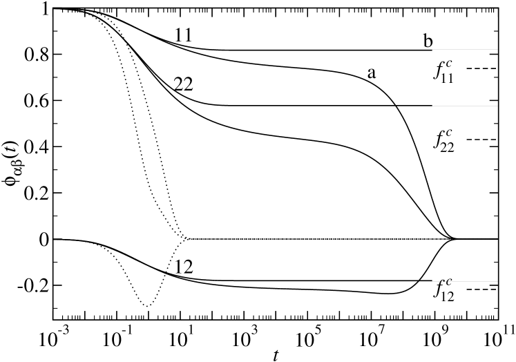
Figure 1: Normalized correlation functions $\phi_{\alpha\beta}(q,t)=\left(S^{-1/2}(q)\Phi(q,t)S^{-1/2}(q)\right)_{\alpha\beta}$ for a binary hard-sphere mixture with diameter ratio $d_{\text{B}}/d_{\text{A}}=0.6$, packing fraction of B-particles $\varphi_{\text{B}}/\varphi=0.2$, wave vector $q=6.2/d_{\text{A}}$, calculated from Eq. (7); details see text. The labels 11, 12, and 22 indicate the three independent matrix elements, and labels a and b correspond to total packing fractions $\varphi=0.5195$ and $0.525$, respectively. Here, $\varphi=(\pi N/6V)(x_{\text{A}}d_{\text{A}}^{3}+x_{\text{B}}d_{\text{B}}^{3})$, with $x_{\alpha}=N_{\alpha}/N$ being the number concentrations. The dashed horizontal lines indicate the long-time limit for $\varphi=\varphi^{c}\approx 0.519608$, and the dotted curves correspond to an exponential decay as described in the text.

Typical solutions to the MCT equations appear in Fig. 1. We chose as the simplest case a binary mixture of hard spheres. Then the state of the system is determined by three numbers, which we take to be the total packing fraction, $\varphi=\varphi_{\text{A}}+\varphi_{\text{B}}$, the diameter ratio $\delta=d_{\text{B}}/d_{\text{A}}$, and the packing contribution of the second species, $\varphi_{\text{B}}/\varphi$. Here, the species are labeled with subscripts A and B, and $\varphi_{\alpha}=(\pi d_{\alpha}^{3}/6)(N_{\alpha}/V)$ are the partial volumes occupied by each species. To calculate the MCT vertex, Eq. (13), one needs to know the static structure factor of the system, as well as static three-particle correlation functions. For the latter, to our knowledge, no analytic expressions are available, and thus we follow the commonly applied approximation through two-particle correlations Fuchs and Latz (1993). The former shall be approximated using the well-known Percus-Yevick (PY) approximation to the Ornstein-Zernike integral equation. Within this framework, “PY-exact” solutions are available Lebowitz and Rowlinson (1964). As was already mentioned in connection with Eq. (13), the approximations involved in evaluating the vertex are of no importance for the mathematical aspects of the solutions we wish to demonstrate.

Figure 1 shows normalized correlation functions $\phi(q,t)=S^{-1/2}(q)\Phi(q,t)S^{-1/2}(q)$ for a particular wave vector $q=6.2/d_{\text{A}}$. They are numerical solutions of Eq. (7) with $\tau_{\alpha\beta}(q)=1/(q^{2}D^{0}_{\alpha})\delta_{\alpha\beta}$ and $D^{0}_{\alpha}=0.005/R_{\alpha}$, on a grid of 100 wave vectors $q=0.2,\dots 39.8$ with $\Delta q=0.4$. The size ratio and the concentrations are kept fixed at $(\delta,\varphi_{\text{B}}/\varphi)=(0.6,0.2)$, and the total packing fraction is varied as indicated in the figure caption; a procedure corresponding to what has been done in experiment Williams and van Megen (2001). Note that while the two diagonal matrix elements are positive and monotonically decreasing for all times $t$, both needs not be true in general for the off-diagonal elements. For comparison also shown is the suggested starting point of Eq. (15), $\phi^{(0)}(t)=S^{-1/2}\exp[-(S\tau)^{-1}t]S^{1/2}$, which is completely monotone by construction. One notices a drastic slowing down in the relaxation of the correlation functions towards their long-time limits. This demonstrates the dynamics close to a critical point where the Perron-Frobenius eigenvalue $r=1$, which in this system occurs at $\varphi^{c}\approx 0.519608$ and which is the concern of the asymptotic solutions to mode-coupling theory. The solutions for the long-time limit at $\varphi=\varphi^{c}$ as determined from Eq. (25) are included in the figure.

Figure 2: Eigenvalues $e_{\pm}(q,t)$ of $\phi(q,t)$ from Fig. 1 for $\varphi=0.5195$ (all other parameters as given in Fig. 1) as functions of time $t$.

Complete monotonicity requires all eigenvalues of $\phi(t)$ to be positive for all $t$. To demonstrate that our numerical solution is in accordance with this, we show in Fig. 2 the eigenvalues $e_{\pm}(t)$ as functions of time for a fixed total packing fraction. One clearly recognizes the above statement to hold.

A power series in the time domain exists, and at regular points, i.e. for vertices such that the Perron-Frobenius eigenvalue is smaller than unity, also for small frequencies the power series has a nonzero radius of convergence. In particular, the existence of all moments of the density correlation function at regular points, and of a finite radius of convergence for the frequency-domain power series implies the existence of a final exponential relaxation,

$$\Phi(t)-F^{*}={\mathcal{O}}(e^{-\gamma_{0}t})\,.$$ (48)

This holds, since Eq. (43) implies that the measure $a$ in Eq. (3) has an atom of mass $F^{*}$ at $\gamma=0$, is constant for $0<\gamma<\gamma_{0}$, and has a point of increase at $\gamma=\gamma_{0}$ Feller (1971). Thus,

$$\Phi_{\mu\nu}(q,t)=F_{\mu\nu}^{*}(q)+\int_{\gamma_{0}}^{\infty}e^{-\gamma t}\,da_{\mu\nu,q}(\gamma)\,.$$ (49)

The mode-coupling theory for mixtures can also be applied to systems with Newtonian, instead of stochastic, short-time dynamics, e.g. metallic melts. Furthermore, a recent extension of MCT to molecular liquids that treats each molecule as consisting of $s$ constituent sites also leads to substantially the same equations Chong and Götze (2002). Since in these cases, the representation of Eq. (3) through decaying exponentials only will not be valid in general, the proofs presented here cannot readily be applied. Work published for one-component Newtonian systems Haussmann (1990) suggests that existence and uniqueness of the solution, even if it will not be completely monotone, can nevertheless be proven. This has, however, not been done so far.

It is an observation of both theory Franosch et al. (1998) and computer experiment Gleim et al. (1998), that the different short-time behavior does not influence the dynamics at sufficiently long times apart from an overall shift in time scale, given a strong enough coupling such that MCT contributions are important. One then expects the long-time limit of the Newtonian dynamics solutions to exist and to be governed by Eq. (25). Note that the properties of this equation and its maximum fixed point do not depend on the short-time dynamics, nor do the commonly applied asymptotic formulas. Similarly, the prediction of only $A_{\ell}$ singularities as glass transitions will remain valid as long as the linearization of Eq. (25) is irreducible. This can be expected unless some special symmetry will introduce zero-couplings in the vertex, which in principle can happen within the molecular site-site description of Ref. Chong and Götze (2002).

Appendix A Perron Theorem

Let us sketch here for completeness some results generalized from the Perron-Frobenius theorem for irreducible matrices Gantmacher (1974). For a generalization of the complete theorem for positive linear maps on $C^{\star}$ algebras, the reader is referred to Ref. Evans and Høegh-Krohn (1978).

As above, let ${\mathcal{A}}^{M}$ denote the $C^{\star}$ algebra of $M$-vectors of $s\times s$ matrices over $\mathbb{C}$. Consider the positive linear map $\psi$, which maps the set of symmetric, real, positive definite elements ${\mathcal{A}}^{M}_{+}$ onto itself, $\psi[a]\succeq 0$ for $a\succeq 0$. $\psi$ is called irreducible, if there exists some positive, finite number $n$ such that $T[a]\succ 0$ for $a\succeq 0$ and

$$T[a]=(1+\psi)^{n}[a]\,.$$ (50)

If $\psi$ is irreducible, we have that $\psi[a]\succ 0$ if $a\succ 0$.

Now, define a mapping $r:({\mathcal{A}}^{M}_{+},\mathbb{C}^{s})\to\mathbb{R}$ by

$$r(a,v)=\min_{1\leq q\leq M}\frac{(v|\psi_{q}[a]v)}{(v|a_{q}v)}\,,$$ (51)

where $q$ labels the elements of $a\in{\mathcal{A}}^{M}$, $a=(a_{q})_{q=1,\dots M}$, and $(\cdot|\cdot)$ is a scalar product over $\mathbb{C}^{s}$. Furthermore, set $r(a)=\inf_{v\in\mathbb{C}^{s}}r(a,v)=\inf_{v\in\mathbb{S}^{s}}r(a,v)$, where $\mathbb{S}^{s}$ denotes the $s$-dimensional unit sphere, and the latter equation holds since $r(a,\lambda v)$ with $\lambda\in\mathbb{C}$ is independent of $\lambda$.

One immediately checks $r(a)\geq 0$ and

$$\psi[a]\succeq r(a)a\,.$$ (52)

However, $r(a,v)$ is not continuous on $({\mathcal{A}}^{M}_{+},\mathbb{C}^{s})$. Let us define a set

$${\mathcal{B}}:=\{b;b=T[a],a\in{\mathcal{A}}^{M}_{+},\|a\|=1\}\,.$$ (53)

Then, $b\succ 0$ for any $b\in{\mathcal{B}}\subset{\mathcal{A}}^{M}_{+}$. Since $r(b,v)$ is continuous on the closed and compact set $(\mathcal{B},\mathbb{S}^{s})$, it assumes its minimum with respect to $v$. It follows that on $\mathcal{B}$, $r(b)$ fulfills a maximum principle in the sense that it is the maximum $\mathbb{R}$-number for which $\psi[b]\succeq r(b)b$. Furthermore, for $a\in{\mathcal{A}}^{M}_{+}$ and $b=T[a]\in{\mathcal{B}}$ we have $T[\psi(a)-r(a)a]=\psi[b]-r(a)b\succ 0$, and by the maximum principle we get $r(b)\geq r(a)$.

Next define

$$r=\sup_{a\in{\mathcal{A}}^{M}_{+}}r(a)\,.$$ (54)

Since $r(1)>0$, clearly $r>0$. The supremum can be restricted to $b\in\mathcal{B}$ since the above inequality holds. But there, $r(b)$ assumes its maximum, and thus $r$ attains the supremum for some extremal vector $z\succ 0$.

We continue by showing that $r$ indeed is an eigenvalue of $\psi$ and equal to the spectral radius, and that the corresponding eigenvector $z$ is unique, i.e. the eigenvalue is non-degenerate.

Assume, $\psi[z]-rz\succeq 0$ but not the null element. Then $\psi[\hat{z}]-r\hat{z}\succ 0$ with $\hat{z}=T[z]$, but the maximum principle then implies $r(\hat{z})>r$ in contradiction to the definition of $r$. Thus, $r$ is an eigenvalue of $\psi$. Suppose now, there are two eigenvectors $z$, $z^{\prime}$ corresponding to this eigenvalue. We then can find some $\lambda\in\mathbb{R}$ such that $\lambda z-z^{\prime}\succeq 0$ but not strictly positive definite. But this implies $T[\lambda z-z^{\prime}]=(1+r)^{n}(\lambda z-z^{\prime})\succ 0$, in contradiction to the construction of $\lambda$. Thus, the eigenvalue $r$ is non-degenerate.

Now for any $a\in{\mathcal{A}}^{M}_{+}$, define the mapping

$$\sigma[a]=(1/r)z^{-1/2}\psi[z^{1/2}az^{1/2}]z^{-1/2}\,.$$ (55)

Since $\sigma[1]=1$, $\|\sigma\|=1$. Suppose $\psi[u]=\alpha u$ with some $\alpha\in\mathbb{C}$. Write $v=z^{-1/2}uz^{-1/2}$, which gives $\sigma[v]=(\alpha/r)v$. But for any eigenvalue $\lambda$ of $\sigma$, we have $|\lambda|\leq\|\sigma\|$, and thus in particular $|\alpha|\leq r$. Therefore, $r$ is the spectral radius of $\psi$.

References

- Götze and Sjögren (1995) W. Götze and L. Sjögren, J. Math. Analysis and Appl. 195, 230 (1995).
- Williams and van Megen (2001) S. R. Williams and W. van Megen, Phys. Rev. E 64, 041502 (2001).
- Götze (1999) W. Götze, J. Phys.: Condens. Matter 11, A1 (1999).
- Nägele (1996) G. Nägele, Phys. Rep. 272, 215 (1996).
- Gripenberg et al. (1990) G. Gripenberg, S. O. Londen, and O. Staffans, Volterra Integral and Functional Equations, vol. 34 of Encyclopedia of Mathematics and Its Applications (Cambridge University Press, Cambridge, 1990).
- Widder (1946) D. V. Widder, The Laplace Transform (Princeton University Press, Princeton, 1946).
- Boon and Yip (1980) J.-P. Boon and S. Yip, Molecular Hydrodynamics (McGraw-Hill, New York, 1980).
- Hansen and McDonald (1986) J.-P. Hansen and I. R. McDonald, Theory of Simple Liquids (Academic Press, London, 1986), 2nd ed.
- Bengtzelius et al. (1984) U. Bengtzelius, W. Götze, and A. Sjölander, J. Phys. C 17, 5915 (1984).
- Götze (1991) W. Götze, in Liquids, Freezing and Glass Transition, edited by J. P. Hansen, D. Levesque, and J. Zinn-Justin (North Holland, Amsterdam, 1991), vol. Session LI (1989) of Les Houches Summer Schools of Theoretical Physics, pp. 287–503.
- Fuchs and Latz (1993) M. Fuchs and A. Latz, Physica A 201, 1 (1993).
- Götze (1987) W. Götze, in Amorphous and Liquid Materials, edited by E. Lüscher, G. Fritsch, and G. Jacucci (Nijhoff Publishers, Dordrecht, 1987), NATO ASI Series, pp. 34–81.
- Sciortino and Kob (2001) F. Sciortino and W. Kob, Phys. Rev. Lett. 86, 648 (2001).
- Feller (1971) W. Feller, An Introduction to Probability Theory and Its Applications, vol. II (Wiley & Sons, New York, 1971), 2nd ed.
- Gantmacher (1974) F. R. Gantmacher, The Theory of Matrices, vol. II (Chelsea Publishing, New York, 1974).
- Evans and Høegh-Krohn (1978) D. E. Evans and R. Høegh-Krohn, J. London Math. Soc. (2) 17, 345 (1978).
- Arnol’d (1975) V. I. Arnol’d, Russ. Math. Survey 30, 1 (1975).
- Franosch et al. (1997) T. Franosch, M. Fuchs, W. Götze, M. R. Mayr, and A. P. Singh, Phys. Rev. E 55, 7153 (1997).
- Lebowitz and Rowlinson (1964) J. L. Lebowitz and J. S. Rowlinson, J. Chem. Phys. 41, 133 (1964).
- Chong and Götze (2002) S.-H. Chong and W. Götze (2002), eprint cond-mat/0112127.
- Haussmann (1990) R. Haussmann, Z. Phys. B 79, 143 (1990).
- Franosch et al. (1998) T. Franosch, W. Götze, M. R. Mayr, and A. P. Singh, J. Non-Cryst. Solids 235–237, 71 (1998).
- Gleim et al. (1998) T. Gleim, W. Kob, and K. Binder, Phys. Rev. Lett. 81, 4404 (1998).