Effects of Charge Ordering on Spin-Wave of Quarter-Filled
Spin-Density-Wave States

1 Introduction

Organic conductors, tetramethyltetraselenafulvalene (TMTSF) and tetramethyltetrathiafulvalene (TMTTF) salts, ${}^{\hbox{\immediate{\bf{?}},\penalty 1000\hskip 0.91003pt plus 0.70004pt minus 0.70004pt{\bf{?}})}}$ exhibit, due to an interplay of interaction and low dimension, exotic spin-density-wave (SDW) states, which coexist with the charge-density-wave (CDW), e.g., 4$k_{\rm F}$ CDW in TMTTF salt and 2$k_{\rm F}$ CDW in TMTSF salt ($k_{\rm F}$ denotes a Fermi wave number). ${}^{\hbox{\immediate{\bf{?}},\penalty 1000\hskip 0.91003pt plus 0.70004pt minus 0.70004pt{\bf{?}})}}$ These states have been analyzed in terms of the extended Hubbard model with several repulsive interactions. Applying the mean-field theory, it is shown that the interactions with finite-range play a crucial role for the coexistence. The coexistence of SDW with 4$k_{\rm F}$ CDW (2$k_{\rm F}$ CDW) appears when the nearest-neighbor repulsive interaction $V$, (the next-nearest-neighbor repulsive interaction $V_{2}$) becomes large. ${}^{\hbox{\immediate{\bf{?}},\penalty 1000\hskip 0.91003pt plus 0.70004pt minus 0.70004pt{\bf{?}})}}$

The fluctuations around the SDW ground state have been examined extensively by calculating the collective modes within the random phase approximation (RPA). The modes for charge and spin fluctuations in the presence of only on-site repulsive interaction ($U$) were evaluated for the incommensurate SDW ${}^{\hbox{\immediate{\bf{?}},\penalty 1000\hskip 0.91003pt plus 0.70004pt minus 0.70004pt{\bf{?}},\penalty 1000\hskip 0.91003pt plus 0.70004pt minus 0.70004pt{\bf{?}},\penalty 1000\hskip 0.91003pt plus 0.70004pt minus 0.70004pt{\bf{?}},\penalty 1000\hskip 0.91003pt plus 0.70004pt minus 0.70004pt{\bf{?}})}}$ and for the commensurate SDW state at quarter-filling, ${}^{\hbox{\immediate{\bf{?}},\penalty 1000\hskip 0.91003pt plus 0.70004pt minus 0.70004pt{\bf{?}})}}$ where the latter may be relevant to above organic conductors. The commensurability energy induces an excitation gap in the charge excitation where the gap becomes zero at $V=V_{\rm c}$. ${}^{\hbox{\immediate{\bf{?}})}}$ When $V=V_{\rm c}$, a coexistent state of 2$k_{\rm F}$ SDW and 4$k_{\rm F}$ CDW appears ${}^{\hbox{\immediate{?})}}$ and the harmonic potential for the charge fluctuation vanishes. The presence of $V_{2}$ leads to an unusual ground state where 2$k_{\rm F}$ SDW coexists with 2$k_{\rm F}$ CDW and also with 4$k_{\rm F}$ SDW for $V_{2}>V_{\rm 2c}$. ${}^{\hbox{\immediate{?},\penalty 1000\hskip 0.91003pt plus 0.70004pt minus 0.70004pt{\bf{?}})}}$ When $V_{2}=V_{\rm 2c}$, one finds the disappearance of the harmonic potential with respect to the relative motion between the density wave of the up spin and that of the down spin. For large $V_{2}$, a new collective mode with an excitation gap appears where the mode describes the relative motion of density waves with opposite spin followed by amplitude mode of 2$k_{\rm F}$ CDW. The excitation gap vanishes at $V_{2}=V_{\rm 2c}$. ${}^{\hbox{\immediate{\bf{?}})}}$

While the spin-wave modes at quarter-filling was calculated for the conventional Hubbard model, ${}^{\hbox{\immediate{?},\penalty 1000\hskip 0.91003pt plus 0.70004pt minus 0.70004pt{?})}}$ much of their problems is not known in the presence of $V$ and $V_{2}$. The excitation with long-wavelength has been calculated within the RPA for the case of $V\neq 0$ and $V_{2}=0$, ${}^{\hbox{\immediate{\bf{?}})}}$ and for the spin-wave velocity as a function of $V$ or $V_{2}$ ${}^{\hbox{\immediate{\bf{?}})}}$ based on a functional integral formulation. ${}^{\hbox{\immediate{\bf{?}})}}$ The latter has shown that the spin-wave velocity decreases to zero (a finite value) with increasing $V$ ($V_{2}$) when 2$k_{\rm F}$ SDW coexists with 4$k_{\rm F}$ CDW (2$k_{\rm F}$ SDW coexists with 2$k_{\rm F}$ CDW and 4$k_{\rm F}$ SDW). In the path integral method, it remains an open question how to treat the coupling to long-wavelength spin fluctuations. ${}^{\hbox{\immediate{?})}}$

In the present paper, we examine the acoustic and optical spin-wave modes in the presence of $V$ and $V_{2}$ (leading to the charge ordering) for understanding the properties of the several kinds of transverse spin fluctuations of the SDW ordered states coexisting with CDW. We calculate not only the energy dispersion relation of them but also their collective operators within RPA. In §2, the mean-field ground state and the response function are explained for the calculation of the spin-wave modes. In §3, the resulting energy spectrum of them is given in conjunction with the characteristics of their collective coordinates including several spin fluctuation. In addition, the interaction dependence of the spin-wave velocities is shown as a function of $V$ or $V_{2}$. The effect of the charge ordering on the spin-wave is examined and is compared with that obtained by the path integral method. ${}^{\hbox{\immediate{?})}}$ In §4, we discuss the effect of dimerization and analyze the behaviors of the spin-wave velocity in the limit of large $V$ or $V_{2}$ by using an effective Hamiltonian of a spin 1/2 Heisenberg model.

2 Mean-Field Ground State and Response Function

We study a one-dimensional extended Hubbard model at quarter-filling. The Hamiltonian is given by

$$H = -\sum_{\sigma,j}(t-(-1)^{j}t_{\rm d})(C_{j\sigma}^{\dagger}C_{j+1,\sigma}+{\rm h.c.})$$ (2.1)

$${}+H_{\rm{int}}\;\;,$$

$$H_{\rm{int}} = \sum_{j=1}^{N}(Un_{j\uparrow}n_{j\downarrow}+Vn_{j}n_{j+1}+V_{2}n_{j}n_{j+2})\;\;,$$ (2.2)

where $C_{j\sigma}^{\dagger}$ denotes a creation operator of an electron at the $j$-th site with spin $\sigma=(\uparrow,\downarrow)$, and satisfies a periodic boundary condition $C_{j+N,\sigma}^{\dagger}=C_{j\sigma}^{\dagger}$ with the total number of lattice site $N$, $n_{j}=n_{j\uparrow}+n_{j\downarrow}$ and $n_{j\sigma}=C_{j\sigma}^{\dagger}C_{j\sigma}$. The quantity $t$ and $t_{\rm d}$ are the energy of the transfer integral and that of the dimerization. Quantities $U$, $V$ and $V_{2}$ correspond to coupling constants of repulsive interaction for the on-site, the nearest-neighbor site and the next-nearest-neighbor site, respectively. We take $t$ and the lattice constant as unity.

For a quarter-filled band, the mean-fields (MFs) of SDW and CDW are written as ($m=0,1,2$ and 3, and ${\rm sgn}(\sigma)=+(-)$ for $\sigma=\uparrow(\downarrow)$)

$$S_{mQ_{0}} = \frac{1}{N}\sum_{\sigma=\uparrow,\downarrow}\sum_{-\pi<k\leq\pi}{\rm sgn}(\sigma)\left<C_{k\sigma}^{\dagger}C_{k+mQ_{0},\sigma}\right>_{\rm MF}\;\;,$$

$$D_{mQ_{0}} = \frac{1}{N}\sum_{\sigma=\uparrow,\downarrow}\sum_{-\pi<k\leq\pi}\left<C_{k\sigma}^{\dagger}C_{k+mQ_{0},\sigma}\right>_{\rm MF}\;\;,$$ (2.3b)

where $Q_{0}\equiv 2k_{\rm F}=\pi/2$ with $k_{\rm F}(=\pi/4)$ being the Fermi wave number. The $z$-axis is taken as the quantized axis. The expression $<O>_{\rm MF}$ denotes an average of $O$ over the MF Hamiltonian, ${}^{\hbox{\immediate{?})}}$ given by

$$H_{\rm MF} = \sum_{\sigma=\uparrow,\downarrow}\sum_{-\pi<k\leq\pi}\Bigl{[}\Bigl{(}\varepsilon_{k}+\frac{U}{4}+V+V_{2}\Bigr{)}C_{k\sigma}^{\dagger}C_{k\sigma}$$ (2.4)

$${}+\Bigl{\{}\Bigl{(}(\frac{U}{2}-2V_{2})D_{Q_{0}}-{\rm sgn}(\sigma)\frac{U}{2}S_{Q_{0}}\Bigr{)}$$

$$\hskip 14.22636pt{}\times C_{k+Q_{0},\sigma}^{\dagger}C_{k\sigma}+{\rm h.c.}\Bigr{\}}$$

$${}+\Bigl{(}(\frac{U}{2}-2V+2V_{2})D_{2Q_{0}}-{\rm sgn}(\sigma)\frac{U}{2}S_{2Q_{0}}$$

$$\hskip 14.22636pt{}-2{\rm i}t_{\rm d}\sin k\Bigr{)}C_{k\sigma}^{\dagger}C_{k+2Q_{0},\sigma}\Bigr{]}$$

$${}+NU\Bigl{[}-\frac{1}{16}-\frac{1}{2}\Bigl{(}{|D_{Q_{0}}|}^{2}-{|S_{Q_{0}}|}^{2}\Bigr{)}$$

$${}-\frac{1}{4}\Bigl{(}D_{2Q_{0}}^{2}-S_{2Q_{0}}^{2}\Bigr{)}\Bigr{]}+NV\Bigl{(}-\frac{1}{4}+D^{2}_{2Q_{0}}\Bigr{)}$$

$${}+NV_{2}\Bigl{(}-\frac{1}{4}+2{|D_{Q_{0}}|}^{2}-D^{2}_{2Q_{0}}\Bigr{)}\;\;,$$

where $\varepsilon_{k}=-2t\cos k$. The expressions of each MF are given such that $S_{0}=0$, $D_{0}=1/2$, $S_{Q_{0}}=S^{*}_{3Q_{0}}\equiv S_{1}{\rm e}^{{\rm i}\theta}$, $D_{Q_{0}}=D^{*}_{3Q_{0}}\equiv D_{1}{\rm e}^{{\rm i}(\theta-\pi/2)}$, $S_{2Q_{0}}=S^{*}_{2Q_{0}}\equiv S_{2}$ and $D_{2Q_{0}}=D^{*}_{2Q_{0}}\equiv D_{2}$. Quantities $S_{1}(>0)$, $D_{1}(\geq 0)$, $S_{2}$ and $D_{2}$ denote amplitudes for 2$k_{\rm F}$ SDW, 2$k_{\rm F}$ CDW, 4$k_{\rm F}$ SDW and 4$k_{\rm F}$ CDW, respectively. Their values depend on the corresponding ground states. The quantity $\theta$ denotes a phase of SDW. ${}^{\hbox{\immediate{?})}}$

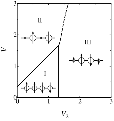
Fig.  1: Phase diagram in the $V$-$V_{2}$ plane for $U=4$ and $t_{\rm d}=0$. ${}^{\hbox{\immediate{?})}}$ Three kinds of states correspond to a pure state of 2$k_{\rm F}$ SDW(I), a state of 2$k_{\rm F}$ SDW and 4$k_{\rm F}$ CDW (II) and a state of 2$k_{\rm F}$ SDW, 2$k_{\rm F}$ CDW and 4$k_{\rm F}$ SDW (III). These states are shown schematically in the region where the arrow (circle) represents the spin (charge) density at each lattice site. The dashed curve denotes a first-order transition between regions II and III.

The ground state has been obtained previously ${}^{\hbox{\immediate{?},\penalty 1000\hskip 0.91003pt plus 0.70004pt minus 0.70004pt{?},\penalty 1000\hskip 0.91003pt plus 0.70004pt minus 0.70004pt{?})}}$ where the phase diagram on the plane of $V_{2}$ and $V$ is shown in Fig. 1. When $V_{2}=0$ and $t_{\rm d}=0$, a pure 2$k_{\rm F}$ SDW state ($\theta=\pi/4$, $\phi=\pi/2$) (I) is found for $V<V_{\rm c}$ ($\simeq 0.34$) and a coexistent state of 2$k_{\rm F}$ SDW and 4$k_{\rm F}$ CDW ($\theta=0$, $\phi=\pi/2$) (II) is found for $V>V_{\rm c}$ ,${}^{\hbox{\immediate{?},\penalty 1000\hskip 0.91003pt plus 0.70004pt minus 0.70004pt{?})}}$ where $\phi=\tan^{-1}(S_{1}/D_{1})$. When $V=0$ and $t_{\rm d}=0$, the pure 2$k_{\rm F}$ SDW state (I) changes to a coexistent state of 2$k_{\rm F}$ SDW, 2$k_{\rm F}$ CDW and 4$k_{\rm F}$ SDW ($\theta=\pi/4$, $\phi<\pi/2$) (III) for $V_{2}>V_{\rm 2c}$ ($\simeq 1.32$). ${}^{\hbox{\immediate{?})}}$ Note that the finite-range interactions $V$ and $V_{2}$ contribute to the appearance of the quantities $D_{1}$ and $D_{2}$. In the following, we use the states I, II and III for those in the regions I, II and III, respectively.

The spin-wave is examined for the above three ground states. The spectrum of the spin-wave modes is calculated from the pole of the response function given by ${}^{\hbox{\immediate{?})}}$

$$\stackrel{{\scriptstyle\leftrightarrow}}{{R}}(q,\omega) = \frac{-1}{2N}\int^{\beta}_{0}{\rm d}\tau\left<T_{\tau}\Phi(q,\tau)\Phi^{\dagger}(q)\right>{\rm e}^{{\rm i}\omega_{n}\tau}{\hbox{$\left|\vbox to0.0pt{}\right.\n@space$}}_{{\rm i}\omega_{n}\rightarrow\omega+{\rm i}0}\;\;,$$

where $\omega_{n}(=2\pi n/\beta)$ and $\beta^{-1}(=k_{\rm B}T)$ denote the Matsubara frequency and temperature, respectively. The components of operator $\Phi^{\dagger}(q)$ consist of the transverse spin fluctuations given by $S_{\alpha m}(q)=\sum_{-\pi<k\leq\pi}\psi_{k}^{\dagger}\sigma_{\alpha}\psi_{k+q+mQ_{0}}$ ($\alpha=x,y$) where $\psi_{k}^{\dagger}=(C^{\dagger}_{k\uparrow},C^{\dagger}_{k\downarrow})$ and $\sigma_{\alpha}$ ($\alpha=x,y$) are Pauli matrices. For the state I ($\theta=\pi/4$) and the state II ($0\leq\theta<\pi/4$ due to $t_{\rm d}$), the operator $\Phi^{\dagger}(q)$ can be taken as ${}^{\hbox{\immediate{?})}}$

$$\Phi^{\dagger}(q)=(S_{x1}^{\dagger}(q),S_{x3}^{\dagger}(q),S_{y0}^{\dagger}(q),S_{y2}^{\dagger}(q))\;\,.$$ (2.6)

We note that, for small $q$, two components $S_{x1}^{\dagger}(q)$ and $S_{x3}^{\dagger}(q)$ are related directly to the transverse spin fluctuation of the SDW with wave numbers $Q_{0}$ and $-Q_{0}$ respectively and that other components of $S_{y0}^{\dagger}(q)$ and $S_{y2}^{\dagger}(q)$ denote the fluctuations correlated with those of the wave numbers 0 and $2Q_{0}$. The coupling to long-wavelength spin fluctuation $S_{y0}^{\dagger}(q)$ gives a renormalization of the spin-wave velocity multiplied by a factor $[1-UN(0)]^{1/2}$ in the weak coupling limit ${}^{\hbox{\immediate{\bf{?}})}}$ where $N(0)$ is the density of state per spin at Fermi level. For the coexistent state of 2$k_{\rm F}$ SDW, 2$k_{\rm F}$ CDW and 4$k_{\rm F}$ SDW (the state III) with the spin modulation with $Q_{0}$ and $2Q_{0}$, one needs to extend the operator $\Phi^{\dagger}(q)$ into that with eight components written as

$$\Phi^{\dagger}(q) = (S_{x1}^{\dagger}(q),S_{x3}^{\dagger}(q),S_{x0}^{\dagger}(q),S_{x2}^{\dagger}(q),$$ (2.7)

$$S_{y1}^{\dagger}(q),S_{y3}^{\dagger}(q),S_{y0}^{\dagger}(q),S_{y2}^{\dagger}(q))\;\,.$$

In addition to $S_{x1}^{\dagger}(q)$ and $S_{x3}^{\dagger}(q)$, the component $S_{x2}^{\dagger}(q)$ for small $q$ is also related directly to the transverse spin fluctuation of the SDW with $2Q_{0}$ while other components comes from coupling to these three components. Operators of eqs. (2.6) and (2.7) act to create the transverse spin fluctuations by raising or lowering the spins within the same sites (i.e., rotation of single electron due to on-site interaction). However, the finite-range interactions induce the transverse spin fluctuations with the spin current (i.e., spin rotation followed by neighboring electrons), which is related to the bond spin-density-wave (BSDW) state. ${}^{\hbox{\immediate{\bf{?}},\penalty 1000\hskip 0.91003pt plus 0.70004pt minus 0.70004pt{\bf{?}})}}$ In the present paper, we neglect the effect of spin current, which is left for the study in the separated paper together with the problem of BSDW. Based on such a consideration, eq. (2) within RPA is calculated as

$$\stackrel{{\scriptstyle\leftrightarrow}}{{R}}^{\rm RPA}(q,\omega) = \frac{\stackrel{{\scriptstyle\leftrightarrow}}{{\Pi}}(q,\omega)}{1+U\stackrel{{\scriptstyle\leftrightarrow}}{{\Pi}}(q,\omega)}\;\;,$$ (2.8)

where the polarization function, $\stackrel{{\scriptstyle\leftrightarrow}}{{\Pi}}(q,\omega)$, is evaluated in terms of the MF Hamiltonian, eq. (2.4).

$$\stackrel{{\scriptstyle\leftrightarrow}}{{\Pi}}(q,\omega) = \frac{-1}{2N}\int^{\beta}_{0}{\rm d}\tau\left<T_{\tau}\Phi(q,\tau)\Phi^{\dagger}(q)\right>_{\rm MF}$$ (2.9)

$$\hskip 42.67912pt{}\times{\rm e}^{{\rm i}\omega_{n}\tau}{\hbox{$\left|\vbox to0.0pt{}\right.\n@space$}}_{{\rm i}\omega_{n}\rightarrow\omega+{\rm i}0}\;\,.$$

The pole of eq. (2.8) determines the excitation spectrum of the collective mode, $\omega_{\gamma}(q)$, i.e.,

$$\det\left(1+U\stackrel{{\scriptstyle\leftrightarrow}}{{\Pi}}(q,\omega_{\gamma}(q))\right) = 0\;\;,$$ (2.10)

where $\gamma=T1$ or $T2$ and $\omega_{T1}$ ($\omega_{T2}$) denotes the acoustic (optical) mode. The eigenvector, $\tilde{\Phi}^{\gamma}(q)$, which describes the collective mode, is obtained by

$$\left(1+U\stackrel{{\scriptstyle\leftrightarrow}}{{\Pi}}(q,\omega_{\gamma}(q))\right)\tilde{\Phi}^{\gamma}(q) = 0\;\,.$$ (2.11)

Actually, in terms of $\Phi(q)$ and $\tilde{\Phi}^{\gamma}(q)$, the operator for the spin-wave with $\omega_{\gamma}(q)$ is written as

$$\eta_{\gamma}(q) = \tilde{\Phi}^{\gamma\dagger}(q)\Phi(q)\;\;,$$ (2.12)

an explicit form of which will be given in the next section. For $\omega\simeq\omega_{\gamma}(q)$, eq. (2.8) is rewritten as ${}^{\hbox{\immediate{?})}}$

$$\stackrel{{\scriptstyle\leftrightarrow}}{{R}}^{\rm RPA}(q,\omega) \simeq \frac{S_{1}^{2}}{2}\frac{\stackrel{{\scriptstyle\leftrightarrow}}{{A^{\gamma}}}(q,\omega_{\gamma}(q))}{\omega^{2}-\omega_{\gamma}^{2}(q)}\;\;,$$ (2.13)

$$\stackrel{{\scriptstyle\leftrightarrow}}{{A^{\gamma}}}(q,\omega_{\gamma}(q)) = \frac{2}{S_{1}^{2}}\frac{{\rm adj}\left(1+U\stackrel{{\scriptstyle\leftrightarrow}}{{\Pi}}(q,\omega_{\gamma}(q))\right)}{\frac{\partial}{\partial(\omega^{2})}\left(\det(1+U\stackrel{{\scriptstyle\leftrightarrow}}{{\Pi}}(q,\omega))\right)}_{\omega\rightarrow\omega_{\gamma}(q)},$$

where the matrix $\stackrel{{\scriptstyle\leftrightarrow}}{{A^{\gamma}}}(q,\omega_{\gamma}(q))$ is proportional to the residue and ${\rm adj}\left(1+U\stackrel{{\scriptstyle\leftrightarrow}}{{\Pi}}(q,\omega_{\gamma}(q))\right)$ is the adjoint matrix. The spectral weight of the collective mode is examined by calculating following diagonal element,

$$A_{m}^{\gamma}(q) \equiv \left|\left(\stackrel{{\scriptstyle\leftrightarrow}}{{A^{\gamma}}}(q,\omega(q))\right)_{mm}/U\right|\!\;\;,\hskip 5.69054pt(m=1,3,0,2)\;\,.$$

When $t_{\rm d}=0$ and $V=V_{2}=0$, one finds that, in the limit of small $U$, $A^{T1}_{1}(0)=A^{T1}_{3}(0)=2\pi v_{\rm F}$ with $v_{\rm F}=\sqrt{2}$ and $A^{T2}_{1}(0)=A^{T2}_{3}(0)=A^{\gamma}_{0}(0)=A^{\gamma}_{2}(0)=0$.

We examine the $V$ (or $V_{2}$) dependence of the velocity of acoustic spin-wave given by

$$v=\lim_{q\rightarrow 0}\frac{\omega_{T1}(q)}{q}\;\;,$$ (2.16)

which is compared with the previous work. ${}^{\hbox{\immediate{?})}}$

3 Spin-Wave Modes

The characteristic properties of the spin-wave modes are examined for the various kinds of SDW ground states, which are given by the states I, II and III. The numerical calculation is performed by taking $U=4$ and $t=1$ where $t_{\rm d}=0$ in this section.

3.1 Effect of $V$

First, we calculate the spin-wave spectrum $\omega_{\gamma}(q)$ as a function of $V$ for $V_{2}=0$. In Fig. 2, the spectrum of both the acoustic and optical spin-wave modes obtained from eq. (2.10) are shown for $V=0$, 0.5, 1.5 and 2.0 with $V_{2}=0$ and $t_{\rm d}=0$ where the state II is obtained for $V>V_{\rm c}$ ($\simeq 0.34$). Our numerical calculation within the visible scale shows that spectrum of the acoustic mode takes a simple sine function form with respect to the wave number $q$, i.e., $\omega_{T1}(q)=\omega_{T1}(Q_{0}/2)\sin(2q)$. The optical mode, $\omega_{T2}(q)$, is well separated from the continuum for the parameters in Fig. 2. The spectrum of the state II is similar to that of the state I.

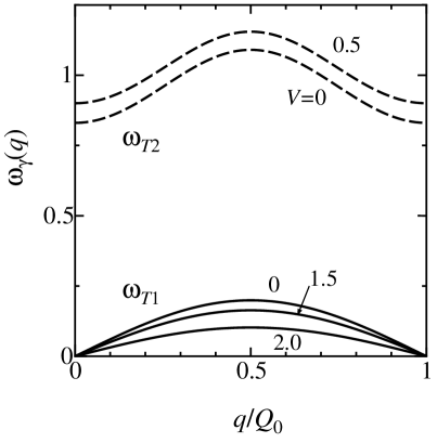
Fig.  2: Excitation spectrum of the spin-wave modes, $\omega_{T1}(q)$ (acoustic mode) and $\omega_{T2}(q)$ (optical mode) for $U=4$, $V_{2}=0$ and $t_{\rm d}=0$.

The spectral weights for the acoustic mode, $A_{m}^{T1}(q)$, are shown in Fig. 3 where $A_{1}^{T1}(q)$ and $A_{3}^{T1}(q)$ ($A_{0}^{T1}(q)$ and $A_{2}^{T1}(q)$) are weights for spin fluctuations of $x$ ($y$) direction with wave numbers $Q_{0}+q$ and $-Q_{0}+q$ ($q$ and $2Q_{0}+q$), respectively. For the spectral weights with $q\simeq 0$ or $Q_{0}$, the dominant weights are given by the fluctuations with $\simeq\pm Q_{0}$ (note that $S_{y0}(Q_{0})=S_{y1}(0)$ and $S_{y2}(Q_{0})=S_{y3}(0)$), as shown for a model with only $U$. ${}^{\hbox{\immediate{?})}}$ Figure 3 indicates that the deviation of the spin orientation arising from the spin-wave changes continuously from the $x$ direction to the $y$ direction when $q$ increases from 0 to $Q_{0}$. It is found that all the weights are suppressed by $V$.

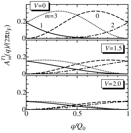
Fig.  3: Normalized spectral weight of the acoustic mode, $A^{T1}_{m}(q)/(2\pi v_{\rm F})$, for $V=0$, 1.5 and 2.0 in Fig. 2.

Fig.  4: Schematics of spin-wave for $q\rightarrow 0$ are shown. (a) acoustic mode in the state I, (b) acoustic mode in the state II, (c) optical mode in the state I and (d) acoustic mode in the state III. The lower part of each figure represents a projection of the spin on the $x$-$y$ plane.

Here we examine the behavior in the limit of small $q$. From the numerical result of eq. (2.11), we found that the eigenvector $\tilde{\Phi}^{T1}(q)$ for the acoustic mode is written as $\tilde{\Phi}^{T1}(q\rightarrow 0)\propto({\rm e}^{{\rm i}\theta},{\rm e}^{-{\rm i}\theta},0,0)$ where $\theta=\pi/4$ for $V<V_{\rm c}$ and $\theta=0$ for $V>V_{\rm c}$. Then, the spin-wave operator of eq. (2.12) in the limit of $q\rightarrow 0$ may be expressed as

$$\eta_{T1}(0) \propto \sum_{j}S^{x}_{j}\cos(Q_{0}r_{j}+\theta)\;\;,$$ (3.1)

where $S^{\alpha}_{j}=\psi^{\dagger}_{j}\sigma_{\alpha}\psi_{j}/2$ and $\psi^{\dagger}_{j}=(C^{\dagger}_{j\uparrow},C^{\dagger}_{j\downarrow})$. Equation (3.1) denotes that the gapless excitation at $q=0$ is described by rotating the spin quantization axis toward $x$ direction uniformly. The spatial dependence is illustrated in Figs. 4(a) and 4(b) for $V<V_{\rm c}$ and for $V>V_{\rm c}$, respectively, which are written simply as $(\nearrow\nearrow\swarrow\swarrow)$ for $V<V_{\rm c}$ and $(\cdot\nearrow\cdot\swarrow)$ for $V>V_{\rm c}$. Similarly, $\omega_{T1}(Q_{0})$, corresponds to the excitation with a uniform rotation toward $y$ direction.

Another spectrum $\omega_{T2}(q)$ of the optical mode has a gap. The corresponding eigenvector $\tilde{\Phi}^{T2}(q)$ is given by $\tilde{\Phi}^{T2}(q\rightarrow 0)\propto({\rm e}^{{\rm i}\theta},-{\rm e}^{-{\rm i}\theta},0,c)$ where $\theta=\pi/4$ and $c>0$ for $V<V_{\rm c}$, and $\theta=0$ and $c=0$ for $V>V_{\rm c}$. Thus, it is found that the spin-wave operator for the optical mode in the limit of $q\rightarrow 0$ is given by

$$\eta_{T2}(0) \propto \sum_{j}\left[2S^{x}_{j}\sin(Q_{0}r_{j}+\theta)+{\rm i}cS^{y}_{j}\cos(2Q_{0}r_{j})\right]\;\,.$$

For $V<V_{\rm c}$, the spatial dependence is shown schematically as $(\nwarrow\>\nearrow\>\searrow\>\swarrow)$ where a plane of $(\nwarrow\>\nearrow)$ is not parallel to that of $(\searrow\>\swarrow)$ due to $c\neq 0$. The explicit spin configuration is illustrated in Fig. 4(c). For $V>V_{\rm c}$, it is given by $(\mbox{$\leftarrow$}\mbox{$\uparrow$}\mbox{$\rightarrow$}\mbox{$\downarrow$})$ where the symbol $\leftarrow$ denotes a component of $S_{j}^{x}$. In Fig. 5, the gap of the optical mode, $\omega_{T2}(0)$, is shown as a function of $V$. The thin dotted curve denotes the bottom of the continuum. With increasing $V$, $\omega_{T2}(0)$ moves into the continuum at the location shown by the arrow, The inset shows the corresponding spectral weight. The spectral weight, $A_{m}^{T2}$ (m=1,3) reduces and becomes zero at $V\simeq 1$ corresponding to the arrow, i.e., above which the optical mode disappears. For $q\rightarrow 0$, the optical mode in the state I contains the fluctuation of $S_{y2}(q)$ in addition to the fluctuations of $S_{x1}(q)$ and $S_{x3}(q)$ while $S_{y2}(q)$ is absent for the mode in the state II.

Fig.  5: $V$ dependence of the gap, $\omega_{T2}(0)$, for $U=4$, $V_{2}=0$ and $t_{\rm d}=0$ where $\omega_{T2}(q)$ disappears at the location shown by the arrow. The dotted curve denotes the bottom of the continuum. In the inset, the corresponding spectral weight, $A^{T2}_{m}(0)/(2\pi v_{\rm F})$ is shown and the weight is zero if not shown explicitly.

Fig.  6: $V$ dependence of the spin-wave velocity $v$, for $U=4$, $V_{2}=0$ and $t_{\rm d}=0$ where the dot-dashed curve denotes the previous result obtained by a path integral method. ${}^{\hbox{\immediate{?})}}$ In the upper inset, $v^{0}$ as a function of $U$ while, $A^{T1}_{m}(0)/(2\pi v_{\rm F})$ corresponding to the main figure is shown in the lower inset.

Now, we examine the spin-wave velocity $v$, which is evaluated by using eq. (2.16). Figure 6 represents the $V$ dependence of $v$ where the dot-dashed curve denotes the result obtained by the path integral method. ${}^{\hbox{\immediate{?})}}$ The quantity $v^{0}$, which stands for the velocity in the case of $U=4$ and $V=V_{2}=t_{\rm d}=0$, is given by $v^{0}=0.39$ ($1.29$) for the solid (dot-dashed) curve. In the upper inset, the $U$ dependence of $v^{0}$ is shown, where the solid curve and dot-dashed curve correspond to those in the main figure. There is a small jump at $V=V_{\rm c}$ due to the discontinuity of $S_{1}$ and $D_{2}$, which occurs only for $t_{\rm d}=0$. ${}^{\hbox{\immediate{?})}}$ With increasing $V(>V_{\rm c})$, $v$ (solid curve) takes a slight hump and decreases to zero more rapidly than that of the dot-dashed curve. The coupling to long-wavelength spin fluctuations was neglected in the path integral method. Therefore, it is found that the velocity is strongly renormalized by the coupling to such a spin fluctuation. The hump is not essential since it disappears for $t_{\rm d}\neq 0$ (see Fig. 10). The behavior of $v$ for large $V$ can be understood as that of spin 1/2 Heisenberg model with the effective exchange interaction $J\sim t^{4}/(UV^{2})$, which is discussed in §4. The lower inset shows the corresponding weights of $A_{m}^{T1}(0)$ ($m=1,3$), which decreases with increasing $V$ in a way similar to $v$.

Here we comment on the fact that the spin-wave velocity as a function of $V$ changes rapidly for $V>V_{\rm c}$ while the velocity remains the same as that of $V=0$ for $V<V_{\rm c}$. The latter behavior of the velocity originates in the present scheme of treating the response function. For the case of $V<V_{\rm c}$, in which the pure 2$k_{\rm F}$ SDW state (I) is realized and the MF is independent of the nearest-neighbor interaction $V$, the quantities $\stackrel{{\scriptstyle\leftrightarrow}}{{\Pi}}(q,\omega)$ in eq. (2.9) and $\stackrel{{\scriptstyle\leftrightarrow}}{{R}}^{\lower 2.84526pt\hbox{RPA}}\!\!(q,\omega)$ in eq. (2.8) do not depend on $V$. If we consider, however, the transverse spin fluctuations with the spin current which come from the term of the nearest-neighbor interaction $V$, it is expected that the corresponding response function $\stackrel{{\scriptstyle\leftrightarrow}}{{R}}^{\lower 2.84526pt\hbox{RPA}}\!\!(q,\omega)$ explicitly includes the interaction $V$ though the extended polarization function $\stackrel{{\scriptstyle\leftrightarrow}}{{\Pi}}(q,\omega)$ is still independent of $V$. Thus, the $V$ dependence of the spin-wave velocity may appear in the state I.

3.2 Effect of $V_{2}$

Next, we calculate the spin-wave mode as a function of $V_{2}$ in the state III by using eqs. (2.7) and (2.10). Figure 7 shows the excitation spectrum of the acoustic mode $\omega_{T1}(q)$ with some choices of $V_{2}$ for $U=4$, $V=0$ and $t_{\rm d}=0$, where the coexistent state of 2$k_{\rm F}$ SDW, 2$k_{\rm F}$ CDW and 4$k_{\rm F}$ SDW is found for $V_{2}>V_{\rm 2c}$ ($\simeq 1.32$). The optical mode $\omega_{T2}(q)$ moves into the continuum leading to a disappearance of the mode for $V_{2}(\,\lower 3.22916pt\hbox{$\buildrel\textstyle>\over{\hbox{\raise 0.86108pt\hbox{$\sim$}}}$}\,1.35)$ being just above $V_{\rm 2c}$. With increasing $V_{2}(>V_{\rm 2c})$, the spectrum $\omega_{T1}(q)$ decreases. We note that the dispersions for $V_{2}=1.5$ and 2.0 is also well described by a relation, $\omega_{T1}(q)=\omega_{T1}(Q_{0}/2)\sin(2q)$.

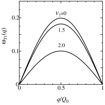
Fig.  7: Excitation spectrum of the spin-wave mode, $\omega_{T1}(q)$, with some choices of $V_{2}$ for $U=4$, $V=0$ and $t_{\rm d}=0$.

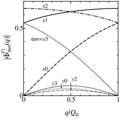
Fig.  8: $q$ dependence of the elements of eigenvector $|\tilde{\Phi}^{T1}(q)|$, corresponding to the case of $V_{2}=2.0$ in Fig. 7.

The corresponding eigenvector $\tilde{\Phi}^{T1}(q)$ for $V_{2}=2.0$ is shown in Fig. 8. For the calculation of the eigenvector in eq. (2.11), we choose seven components except for $S_{y1}(q)$ in $\Phi(q)$ of eq. (2.7) since there are two degenerate modes, i.e., the mode with dominant contribution from $S_{xm}(q)$ and the mode with that from $S_{ym}(q)$. The element $|\tilde{\Phi}^{T1}_{y1}(q)|$ corresponding to $S_{y1}(q)$ is negligibly small, and then the spectrum calculated from seven components is actually nearly the same as that of Fig. 7. It is worthy to note that the mode with small $q$ in the region III of Fig. 1 is composed of not only $S_{xm}(q)$ ($m=1,3$) but also $S_{x2}(q)$ (Fig. 8). Such a feature can be understood by considering the spatial configuration, in which the spin modulation is of type $(\mbox{$\uparrow$}\mbox{$\uparrow$}\mbox{$\downarrow$}\mbox{$\downarrow$})$ (Fig. 1) and the variation of spin moment comes from the presence of 4$k_{\rm F}$ SDW. In this case, the spin-wave operator expressing the gapless excitation at $q\rightarrow 0$ is expected to take a form of

$$\eta_{T1}(0) = \sum_{j}S^{x}_{j}\left[2B_{1}\cos(Q_{0}r_{j}+\theta)+B_{2}\cos(2Q_{0}r_{j})\right]\;\;,$$

which means a uniform rotation toward $x$ direction with keeping the relative angle between the each spin, like $(\mbox{$\nearrow$}\mbox{$\nearrow$}\mbox{$\swarrow$}\mbox{$\swarrow$})$. Here, the coefficients $B_{1}$ and $B_{2}$ satisfies the relation $B_{2}/B_{1}=S_{2}/S_{1}$ according to the spin modulation in the ground state. In eq. (3.2), the term of $B_{2}$ comes from the fluctuation of $S_{x2}(q)$. Actually, our numerical calculation shows that

$$\tilde{\Phi}^{T1}(q){\hbox{$\left|\vbox to0.0pt{}\right.\n@space$}}_{q\rightarrow 0} = \left(\tilde{\Phi}^{T1}_{x1}(q),\tilde{\Phi}^{T1}_{x3}(q),\tilde{\Phi}^{T1}_{x0}(q),\tilde{\Phi}^{T1}_{x2}(q),\right.$$ (3.4)

$${}\left.\tilde{\Phi}^{T1}_{y3}(q),\tilde{\Phi}^{T1}_{y0}(q),\tilde{\Phi}^{T1}_{y2}(q)\right){\hbox{$\left|\vbox to0.0pt{}\right.\n@space$}}_{q\rightarrow 0}$$

$$\propto {}\left({\rm e}^{{\rm i}\theta},\>{\rm e}^{-{\rm i}\theta},\>0,\>c^{\prime},\>0,\>0,\>0\right)\;\;,$$

where $\theta=\pi/4$ and $c^{\prime}=|\tilde{\Phi}^{T1}_{x2}(0)|/|\tilde{\Phi}^{T1}_{x1}(0)|=S_{2}/S_{1}$ ($\simeq 1.2$ for $V_{2}=2.0$). The spatial dependence of this spin-wave is explicitly illustrated in Fig. 4(d).

Fig.  9: $V_{2}$ dependence of $v$, for $U=4$, $V=0$ and $t_{\rm d}=0$. The dot-dashed curve denotes the previous result obtained by a path integral method. ${}^{\hbox{\immediate{?})}}$

The spin-wave velocity $v$ corresponding to that in Fig. 7 is shown as a function of $V_{2}$ in Fig. 9 (solid curve). The dot-dashed curve denotes the result obtained previously by the path integral method. With increasing $V_{2}(>V_{\rm 2c})$, the solid curve decreases to zero rapidly while the dot-dashed curve tends to a finite value ($v\rightarrow t$) for large $V_{2}$. ${}^{\hbox{\immediate{?})}}$ Thus the present RPA calculation indicates the importance of the couplings to long-wavelength spin fluctuations, which has been neglected in the previous path integral method. The behavior in the limit of large $V_{2}$ will be discussed in the next section.

4 Discussions

We have examined spin-wave modes in the presence of charge ordering, which exhibits a clear effect of suppressing the spin-wave velocity even without dimerization ($t_{\rm d}=0$). Since the dimerization enhances the effect of the repulsive interaction, one may expect further suppression of the spin-wave velocity by adding the dimerization. In this section, we discuss such an effect of dimerization ($t_{\rm d}\not=0$) together with the limiting behavior of large $V$ or $V_{2}$.

First, we plot the velocity $v$ as a function of $V$ in Fig. 10, with the fixed $t_{\rm d}=0$, 0.1, 0.3 and 0.5 ($U=4$ and $V_{2}=0$). The dimerization $t_{\rm d}$ has an effect of reducing the velocity, which is qualitatively consistent with the result of the path integral method. ${}^{\hbox{\immediate{?})}}$ The $V$ dependence of $v$ in the region II of Fig. 1 can be fitted by a dotted curve, which is proportional to $(t^{2}-t_{\rm d}^{2})/(UV^{2})$. We analyze such a case by noting that the ground state with the spin and charge modulation given by $(0,\uparrow,0,\downarrow,0)$ and $(0,1,0,1)$ already shows up for $V\,\lower 3.22916pt\hbox{$\buildrel\textstyle>\over{\hbox{\raise 0.86108pt\hbox{$\sim$}}}$}\,3$ even if $t_{\rm d}\neq 0$. In this state II, the antiferromagnetic exchange coupling between the up and down spins is induced by the process of the fourth order of the transfers $t\pm t_{\rm d}$ leading the effective Hamiltonian as

$$H^{\rm eff}_{\rm I\!I} \sim J_{\rm I\!I}\sum^{N/2}_{j=1}{\mbox{\boldmath$S$}}_{2j}\cdot{\mbox{\boldmath$S$}}_{2j+2}\;\;,$$ (4.1a)

$$J_{\rm I\!I} = \frac{a_{\rm I\!I}(t^{2}-t_{\rm d}^{2})^{2}}{UV^{2}}\;\;,$$ (4.1b)

where $a_{\rm I\!I}=12$ and ${\mbox{\boldmath$S$}}_{j}=(S^{x}_{j},S^{y}_{j},S^{z}_{j})$ with $S_{j}^{\alpha}=\psi^{\dagger}_{j}\sigma_{\alpha}\psi_{j}/2$ $(\psi^{\dagger}_{j}=(C^{\dagger}_{j\uparrow},C^{\dagger}_{j\downarrow}))$. This expression of $J_{\rm I\!I}$ with $a_{\rm I\!I}=6$ has been obtained by Mori and Yonemitsu. ${}^{\hbox{\immediate{?})}}$ From eq. (4.1a), the spin-wave dispersion is given by $\omega(q)=J_{\rm I\!I}\sin(2q)$ and then the spin-wave velocity is given by $v=2J_{\rm I\!I}$. By comparing $v=2J_{\rm I\!I}$ with the velocity calculated from eq. (2.16) in the inset of Fig. 10, we found $a_{\rm I\!I}\simeq 1.6$. Such a value of $a_{\rm I\!I}$ differs appreciably from that of the effective Hamiltonian although one obtains a good coincidence between them for the case at half-filling. ${}^{\hbox{\immediate{\bf{?}})}}$ It is not yet clear at present why it is complicated to estimate quantitatively by the effective Hamiltonian at quarter-filling.

Fig.  10: $V$ dependence of $v$, for $U=4$, $V_{2}=0$ and the fixed $t_{\rm d}=0$, 0.1, 0.3 and 0.5. The dotted curves represent $v=2J_{\rm I\!I}=2a_{\rm I\!I}(t^{2}-{t_{\rm d}}^{2})^{2}/(UV^{2})$, where $a_{\rm I\!I}\simeq 1.6$ is estimated from the inset.

Fig.  11: $V_{2}$ dependence of $v$, for $U=4$, $V=0$ and the fixed $t_{\rm d}=0$, 0.1, 0.3 and 0.5. The dotted curves represent $v=2\sqrt{{J}_{\rm I\!I\!I}{J}^{\prime}_{\rm I\!I\!I}}\simeq 1.6\times 2(t^{2}-{t_{\rm d}}^{2})^{2}/(UV_{2}^{2})$, which is estimated from the inset.

Next, we examine $V_{2}$ dependence of $v$ with some choices of $t_{\rm d}$, which is shown in Fig. 11. With increasing $t_{\rm d}$, $v$ is suppressed monotonically in the region III (Fig. 1). For arbitrary value of $t_{\rm d}$ in the region III, $v$ can be well fitted by a dotted curve which is proportional to $(t^{2}-t_{\rm d}^{2})^{2}/(UV_{2}^{2})$. Such a behavior can be also analyzed in terms of the following effective Hamiltonian. In this case, the spin and charge modulation in the ground state is given by $(0,\uparrow,\downarrow,0,0,\uparrow,\downarrow,0)$ and $(0,1,1,0,0,1,1,0)$, respectively. The exchange coupling between the spins of $(\uparrow,\downarrow)$ mainly comes from the second process of the transfer, while that between the spins of $(\downarrow,0,0,\uparrow)$ comes from the sixth order process. Thus, the effective Hamiltonian for large $V_{2}$ can be expressed as the Heisenberg model with the alternating interactions, i.e.,

$$H^{\rm eff}_{\rm I\!I\!I} \sim \sum^{N/4}_{j=1}\left(J_{\rm I\!I\!I}{\mbox{\boldmath$S$}}_{4j-2}\cdot{\mbox{\boldmath$S$}}_{4j-1}+J^{\prime}_{\rm I\!I\!I}{\mbox{\boldmath$S$}}_{4j-1}\cdot{\mbox{\boldmath$S$}}_{4j+2}\right)\;\;,$$

$$J_{\rm I\!I\!I} = \frac{a_{\rm I\!I\!I}(t-t_{\rm d})^{2}}{U}\!\!\;\;,$$ (4.2b)

$$J^{\prime}_{\rm I\!I\!I} = \frac{a_{\rm I\!I\!I}^{\prime}(t+t_{\rm d})^{2}(t^{2}-t_{\rm d}^{2})^{2}}{UV_{2}^{4}}\;\;,$$ (4.2c)

where $a_{\rm I\!I\!I}=4$ and $a_{\rm I\!I\!I}^{\prime}=1$. In this case, one can find the expression of the spin-wave dispersion (Appendix) as , $\omega(q)=\sqrt{J_{\rm I\!I\!I}J^{\prime}_{\rm I\!I\!I}}\sin(2q)$, where $\sqrt{J_{\rm I\!I\!I}J^{\prime}_{\rm I\!I\!I}}=\sqrt{a_{\rm I\!I\!I}a_{\rm I\!I\!I}^{\prime}}(t^{2}-t_{\rm d}^{2})^{2}/(UV_{2}^{2})$. By comparing $v=2\sqrt{J_{\rm I\!I\!I}J^{\prime}_{\rm I\!I\!I}}$ with the numerical result in the inset of Fig. 11, we find $\sqrt{a_{\rm I\!I\!I}a_{\rm I\!I\!I}^{\prime}}\simeq 1.6$, which is compatible with that of the effective Hamiltonian, i.e., 2.

In summary, we have calculated the spin-wave excitations for a one-dimensional model with a quarter-filled band to investigate the effects of the nearest ($V$) and next-nearest-neighbor ($V_{2}$) interactions on them. From the dispersion relations for spin-wave modes in the coexistent state of SDW and CDW, we found that the spectrum of acoustic mode and then the spin-wave velocity are reduced by CDW (induced by $V$ or $V_{2}$) and that the spin-wave in the coexistent state for large $V$ or $V_{2}$ could be described by spin 1/2 antiferromagnetic Heisenberg models with the effective exchange coupling.

5 Spin-Wave of the Heisenberg Antiferromagnets

By taking four lattice sites as a unit cell and introducing the sublattice $A$ and $B$, the Hamiltonian of eqs. (4.1a) and (4.2a) can be rewritten as

$$H^{\rm eff} = \sum^{N/4}_{l=1}\left(J{\mbox{\boldmath$S$}}_{B,l}\cdot{\mbox{\boldmath$S$}}_{A,l}+J^{\prime}{\mbox{\boldmath$S$}}_{B,l}\cdot{\mbox{\boldmath$S$}}_{A,l+1}\right)\;\;,$$ (5.1)

where $J=J^{\prime}=J_{\rm I\!I}$ for eq. (4.1a), and $J=J_{\rm I\!I\!I}$ and $J^{\prime}=J^{\prime}_{\rm I\!I\!I}$ for eq. (4). By using the Holstein-Primakoff transformation,

$$S^{z}_{A,l} = 1/2-a^{\dagger}_{l}a_{l}\;\;,$$ (5.2)

$$S^{+}_{A,l} = S^{x}_{A,l}+{\rm i}S^{y}_{A,l}=(1-a^{\dagger}_{l}a_{l})^{1/2}a_{l}\;\;,$$ (5.3)

$$S^{-}_{A,l} = S^{x}_{A,l}-{\rm i}S^{y}_{A,l}=a^{\dagger}_{l}(1-a^{\dagger}_{l}a_{l})^{1/2}\;\;,$$ (5.4)

$$S^{z}_{B,l} = -1/2+b^{\dagger}_{l}b_{l}\;\;,$$ (5.5)

$$S^{+}_{B,l} = S^{x}_{B,l}+{\rm i}S^{y}_{B,l}=b^{\dagger}_{l}(1-b^{\dagger}_{l}b_{l})^{1/2}\;\;,$$ (5.6)

$$S^{-}_{B,l} = S^{x}_{B,l}-{\rm i}S^{y}_{B,l}=(1-b^{\dagger}_{l}b_{l})^{1/2}b_{l}\;\;,$$ (5.7)

eq. (5.1) up to the second order with respect to $a_{q}$ and $b_{q}$ is given by

$$H^{\rm eff} \simeq \frac{1}{2}\sum_{q}\left[(J+J^{\prime})\left(b^{\dagger}_{q}b_{q}+a^{\dagger}_{q}a_{q}\right)\right.$$ (5.8)

$$\left.{}+(J+J^{\prime}{\rm e}^{-{\rm i}4q})b^{\dagger}_{q}a^{\dagger}_{q}+(J+J^{\prime}{\rm e}^{{\rm i}4q})b_{q}a_{q}\right]\;\;,$$

where the constant term is subtracted and the boson operators $a^{\dagger}_{q}$ and $b^{\dagger}_{q}$ are given by

$$a^{\dagger}_{q} = (N/4)^{-1/2}\sum_{l}{\rm e}^{{\rm i}qR_{l}}\>a^{\dagger}_{l}\;\;,$$ (5.9)

$$b^{\dagger}_{q} = (N/4)^{-1/2}\sum_{l}{\rm e}^{-{\rm i}qR_{l}}\>b^{\dagger}_{l}\;\,.$$ (5.10)

By applying the Bogoliubov transformation to eq.(5.8), the spin-wave dispersion, $\omega(q)$, is obtained from

$$\det\left(\begin{array}[]{cc}\omega(q)-(J+J^{\prime})/2&-(J+J^{\prime}{\rm e}^{{\rm i}4q})/2\\ (J+J^{\prime}{\rm e}^{-{\rm i}4q})/2&\omega(q)+(J+J^{\prime})/2\end{array}\right) = 0\;\,.$$ (5.13)

Equation eq. (5.13) leads to the spin-wave dispersion for the Hamiltonian (5.1) as

$$\omega(q) = \sqrt{JJ^{\prime}}\sin(2q)\;\;,$$ (5.15)

where $\omega(q)=J_{\rm I\!I}\sin(2q)$ for the Hamiltonian (4.1a) and $\omega(q)=\sqrt{J_{\rm I\!I\!I}J^{\prime}_{\rm I\!I\!I}}\sin(2q)$ for the Hamiltonian (4).

References

- [1] D. Jérome and H. J. Schulz: Adv. Phys. 31 (1982) 299.
- [2] T. Ishiguro, K. Yamaji and G. Saito: Organic Superconductors (Springer-Verlag, Berlin, 1998).
- [3] J. P. Pouget and S. Ravy: J. Phys. I (France) 6 (1996) 1501; Synth. Met. 85 (1997) 1523.
- [4] S. Kagoshima, Y. Saso, M. Maesato, R. Kondo and T. Hasegawa: Solid State Commun. 110 (1999) 479.
- [5] H. Seo and H. Fukuyama: J. Phys. Soc. Jpn. 66 (1997) 1249.
- [6] N. Kobayashi, M. Ogata and K. Yonemitsu: J. Phys. Soc. Jpn. 67 (1998) 1098.
- [7] Y. Kurihara: J. Phys. Soc. Jpn. 51 (1982) 2123.
- [8] S. Takada: J. Phys. Soc. Jpn. 53 (1984) 2193.
- [9] Y. Kurihara: J. Phys. Soc. Jpn. 53 (1984) 2391.
- [10] G.C. Psaltakis: Solid State Commun. 51 (1984) 535.
- [11] K. Maki and A. Virosztek: Phys. Rev. B 36 (1987) 511.
- [12] Y. Suzumura and N. Tanemura: J. Phys. Soc. Jpn. 64 (1995) 2298.
- [13] N. Tanemura and Y. Suzumura: Prog. Theor. Phys. 96 (1996) 869.
- [14] Y. Suzumura: J. Phys. Soc. Jpn. 66 (1997) 3244.
- [15] Y. Tomio and Y. Suzumura: J. Phys. Soc. Jpn. 69 (2000) 796.
- [16] Y. Tomio and Y. Suzumura: J. Phys. Soc. Jpn. 70 (2001) 2884.
- [17] M. Mori and K. Yonemitsu: Mol. Cryst. Liq. Cryst. 343 (2000) 221.
- [18] Y. Tomio, N. Dupuis and Y. Suzumura: Phys. Rev. B 64 (2001) 125123.
- [19] K. Sengupta and N. Dupuis: Phys. Rev. B 61 (2000) 13493.
- [20] D. Poilblanc and P. Lederer: Phys. Rev. B 37 (1988) 9650; ibid. 37 (1988) 9672.
- [21] G. I. Japaridze: Phys. Lett. A 201 (1995) 239.
- [22] M. Nakamura: Phys. Rev. B 61 (2000) 16377.
- [23] N. Tanemura and Y. Suzumura: J. Phys. Soc. Jpn. 64 (1995) 2158.