[

Orbital Zeeman effect: Signature of a massive spin wave mode in ferromagnetism

Abstract

By deriving the quantum hydrodynamic equations for an isotropic single-band ferromagnet in an arbitrary magnetic field, we find that a massive mode recently predicted splits under the action of the field. The splitting is a peculiarity of charged fermions and is linear in the field to leading order in $q$ bearing resemblance to the Zeeman effect in this limit, and providing a clear signature for the experimental observation of this mode.

] Magnetism in solids has been one of the most studied subjects in physics for the past decades. In particular the behavior of propagating spin waves in metallic materials has now a long list of contributions in the literature. Spin waves in ferromagnetic materials were first predicted by Bloch[1] and Slater[2] and later observed in iron by Lowde.[3] These first theories were constructed based on lattice models of local moments. Predictions for spin waves using Fermi liquid theory[4] were first made by Silin for paramagnetic systems.[5] Paramagnetic spin-waves were found to propagate only under an applied magnetic field. Abrikosov and Dzyaloshinskii[6] were the first to develop a theory of itinerant ferromagnetism based on Landau’s theory of Fermi liquids. Although correct at the phenomenological level, the microscopic foundations for this theory were estabilished only much later by Dzyaloshinskii and Kondratenko.[7]

In this paper we derive the hydrodynamic equations of the ferromagnetic Fermi liquid theory (FFLT) for a finite magnetic field and show that an intrisic degeneracy of a recently predicted massive mode[8] exists and is lifted under the external field, similarly to the Zeeman splitting of a single spin in a magnetic field. Underneath this effect we identify the breaking of chiral symmetry by the external magnetic field in the case of charged fermions, which relates to the orbital motion developed under the Lorentz force. Besides being a clear signature of the massive mode, it is suggested that quantization of this mode will lead to a system of massive magnons with “up” and “down” states that split under an external field. We estimate the values for the fields where the effect will be observed in typical weak ferromagnets.

For isotropic metals, the equations describing dynamics of paramagnetic spin waves are similar to the ones that result from FFLT in the small moments limit. This is expected since in this limit quasi-particles can be defined and one recovers the kinetic behavior of ordinary Fermi liquid theory. However, FFLT rests on the assumption of a quite different, symmetry-broken, ground state and the resulting spin waves propagate with no external magnetic field present. The Goldstone mode associated with spontaneously broken spin rotation invariance has been the paradigm of spin-waves in an isotropic single band ferromagnet and can be derived from FFLT (as well as from lattice models). However, FFLT contains spin-wave modes that have not yet been observed, as pointed out in Ref.[8], where the proper hydrodynamics and parameters for the propagation of the lowest in energy of these modes have been studied. Such mode is not a Goldstone mode, hence its dispersion may in principle be gapped for $q=0$. Indeed, for low $q$ and zero external magnetic field, its dispersion has been shown to be of the form $\omega=\omega_{1}^{+}-\alpha q^{2}$,[9] and propagation is possible only in the quantum hydrodynamic regime (at temperatures for which collisions are almost absent). This is in contrast to the Goldstone mode which is purelly quadratic and also propagates at collision dominated temperatures.[10] Propagation of the massive mode also requires that the interactions have some finite amplitude with $p$-wave symmetry. Lack of observation of such a mode in neutron scattering experiments can be attributed to the low spectral weight the mode carries at small $q$ ($\sim q^{2}$ when rated against the Goldstone mode), however indirect signs of its existence have already been observed.[8]

We begin our derivation by writing the equal time propagator for a system of interacting fermions, $G_{\sigma_{1}\sigma_{2}}({\bf r}_{1}{\bf r}_{2})\equiv\langle a^{\dagger}_{\sigma_{1}}({\bf r}_{1})a_{\sigma_{2}}({\bf r}_{2})\rangle$, where $a$ is the usual fermion anihilation Heisenberg operator and the average is taken with a ferromagnetic ground state. The equation of motion for $G$ is, in spin space, $\partial_{t}G({\bf r}_{1}{\bf r}_{2})+({i}/{\hbar})\int d{\bf r^{\prime}}[{\cal H}({\bf r}_{1}{\bf r}^{\prime})G({\bf r}^{\prime}{\bf r}_{2})-G({\bf r}_{1}{\bf r}^{\prime}){\cal H}({\bf r}^{\prime}{\bf r}_{2})]=g[G],$ where ${\cal H}$ is the interaction Hamiltonian and the functional $g[G]$ is the full time-derivative of $G$. Following an usual script, one turns to a mixed ${\bf r}$ - ${\bf p}$ representation by defining ${\cal H}_{\bf p}({\bf r})=\int d{\bf r^{\prime}}e^{-i{\bf p}\cdot{\bf r^{\prime}}/\hbar}{\cal H}({\bf r}+{\bf r}^{\prime}/2,{\bf r}-{\bf r^{\prime}}/2)$, and likewise for ${\cal N}_{\bf p}({\bf r})$, which brings the equation of motion to the form

$$\partial_{t}{\cal N}_{\bf p}({\bf r})+\int D\tau\left[{\cal H}_{{\bf p^{\prime}}+\hbar{\bf k}/2}({\bf r^{\prime}}+\hbar{\bf s}/2){\cal N}_{\bf p^{\prime}}({\bf r^{\prime}})\right.$$ (1)

$$- \left.{\cal N}_{\bf p^{\prime}}({\bf r^{\prime}}){\cal H}_{{\bf p^{\prime}}-\hbar{\bf k}/2}({\bf r^{\prime}}-\hbar{\bf s}/2)\right]=J[{\cal N}_{\bf p}],$$ (2)

where $D\tau\equiv id{\bf r^{\prime}}d{\bf s}d{\bf p^{\prime}}d{\bf k}e^{i[({\bf p^{\prime}}-{\bf p})\cdot{\bf s}+({\bf r}-{\bf r^{\prime}})\cdot{\bf k}]}/(2\pi)^{6}\hbar$. Expanding Eq.(2) in ${\bf s}$ and ${\bf k}$ yields a formal series in $\hbar$,

$$\partial_{t}{\cal N}_{\bf p}({\bf r})-J [{\cal N}_{\bf p}]=\sum_{n,m=0}^{\infty}\frac{(-1)^{n}}{2}\left(\frac{i\hbar}{2}\right)^{n+m-1}$$ (4)

$$\times\prod_{j=1}^{n}\prod_{l=1}^{m}\frac{\partial^{2}}{\partial r_{\alpha_{j}}\partial p_{\beta_{l}}}\left[\frac{\partial^{2}{\cal H}_{\bf p}({\bf r})}{\partial r_{\beta_{l}}\partial p_{\alpha_{j}}},{\cal N}_{\bf p}({\bf r})\right]_{\pm},$$

where we have (anti) commutation if $m+n$ is (odd) even and sumation over repeated Greek indices.

It is clear from this expression that the repeated action of the derivatives on the fluctuating fields generate coefficients that are higher order in $q$ for higher powers of $\hbar$. If we keep terms up to first order in $q$,

$$\partial_{t}{\cal N}_{\bf p}({\bf r})+\frac{i}{\hbar}\left[{\cal H}_{\bf p}({\bf r})\right.,{\cal N}_{\bf p} \left.({\bf r})\right]-\frac{1}{2}\left\{{\cal H}_{\bf p}({\bf r}),{\cal N}_{\bf p}({\bf r})\right\}$$ (5)

$$+\frac{1}{2} \left\{{\cal N}_{\bf p}({\bf r}),{\cal H}_{\bf p}({\bf r})\right\}=J[{\cal N}_{\bf p}],$$ (6)

where square braces indicate the usual commutator while curly braces are Poisson brackets. Therefore, keeping first order in $q$ leads to the same result obtained by dropping terms in the series that are explicitly ${\cal O}(\hbar^{2})$. However, ${\cal H}_{\bf p}({\bf r})$ is itself a function of $\hbar$, which disables, at this point, comparison with a semi-classical approach.

For the ferromagnetic Fermi liquid there are two distinct underlying scenarios that we call (following Ref.[8]) classical and quantum spin hydrodynamics. We want here to discuss in a general way the origin of these two regimes. For this purpose, it should be recalled that the equilibrium density matrix for a ferromagnetic state is written in the quite general form,[6]

$${\cal N}^{0}_{{\bf p}\sigma\sigma^{\prime}}=n^{0}_{\bf p}\delta_{\sigma\sigma^{\prime}}+\eta({\bf p}){\rm\bf m}_{0}\cdot{\bm{\tau}}_{\sigma\sigma^{\prime}},$$ (7)

where ${\bm{\tau}}$ are Pauli matrices and ${\rm\bf m}_{0}$ is the equilibrium magnetization density, which is a conserved quantity of the ferromagnetic Hamiltonian. From this it is clear that the commutator in (6) is zero unless there are fluctuations about equilibrium.

At high temperatures, thermal fluctuations dominate and this commutator remains irrelevant. The remaining “classical” terms lead to the known Bloch-like hydrodynamics for the Goldstone mode. This regime is refered to as “classical spin hydrodynamics.”

At low temperatures quantum fluctuations dominate, and the commutator in (6) becomes important. It remains finite as long as the fluctuations contain, besides the usual Goldstone-mode, contributions from non conserved quantities as it is the case of spin-current, whose oscillations give rise to the gapped mode studied in Ref.[8], where this regime has been called “quantum spin hydrodynamics.”

The crossover temperature for these two regimes has been found to scale with $(\omega_{1}^{+})^{1/2}$, where $\omega_{1}^{+}\equiv 2|{\rm\bf m}_{0}|(F_{1}^{a}/3-F_{0}^{a})/\hbar N(0)$ is the gap, $F_{\ell}^{(a)s}$ are the usual dimensionless spin (anti) symmetric interaction parameters, and $N(0)$ is the density of states at the Fermi surface.

The preceding discussion is general and establishes the origin of the massive mode. We now turn to the small moments limit, where kinetic equations can be amenably derived. In this limit, we write the effective quasiparticle Hamiltonian and density matrix respectively as ${\cal H}_{{\bf p}\sigma\sigma^{\prime}}({\bf r})=\epsilon_{\bf p}({\bf r})\delta_{\sigma\sigma^{\prime}}+{\bf h}_{\bf p}({\bf r})\cdot{\bm{\tau}}_{\sigma\sigma^{\prime}},$ and ${\cal N}_{{\bf p}\sigma\sigma^{\prime}}({\bf r})=n_{\bf p}({\bf r})\delta_{\sigma\sigma^{\prime}}+{\bm{\sigma}}_{\bf p}({\bf r})\cdot{\bm{\tau}}_{\sigma\sigma^{\prime}}$. These forms for the Hamiltonian and density immediately give

$$\frac{i}{\hbar}\left[{\cal H}_{\bf p}({\bf r}),{\cal N}_{\bf p}({\bf r})\right]=\frac{2}{\hbar}\left({\bm{\sigma}}_{\bf p}({\bf r})\times{\bf h}_{\bf p}({\bf r})\right)\cdot{\bm{\tau}}.$$ (8)

Here the internal field is given by

$${\bf h}_{\bf p}({\bf r})=-\frac{\gamma\hbar}{2}{\bf H}+\frac{2\pi^{2}\hbar^{2}}{m^{*}k_{F}}\sum_{{\bf p^{\prime}}\ell}F_{\ell}^{a}P_{\ell}({\hat{\bf p}}\cdot{\hat{\bf p}^{\prime}}){\bm{\sigma}}_{\bf p^{\prime}}({\bf r}),$$ (9)

where $P_{\ell}$ are Legendre polynomials, ${\bf H}$ is an external magnetic field, and all coupling constants are $\hbar$ independent. We see then from Eqs.(8) and (9) that the commutator of Eq.(6) gives two contributions: a zero-th order term in $\hbar$ which is just the (Larmor) precession of the internal magnetization and a first order term in $\hbar$ that is the precession about the field generated internally. Carefull examination of Eq.(4) shows that this term is the $only$ first order term in $\hbar$ of the series. That is, provided that the effective Hamiltonian is of the Fermi liquid type, the long wavelength limit is equivalent to a Wentzel-Kramers-Brillouin or (eikonal) semi-classical approximation.

We want now to have the Lorentz-force operator explicitly factorized. This is achieved by rewriting Eq.(6) in a gauge transformed “frame” for which ${\bf A}=0$. Also, to leading order in the fluctuations, the non-commuting parts of the Poisson brackets can be dropped, giving

$$\partial_{t}{\cal N}_{\bf p}({\bf r})+\frac{i}{\hbar} \left[{\cal H}_{\bf p}({\bf r}),{\cal N}_{\bf p}({\bf r})\right]+\left\{{\cal N}_{\bf p}({\bf r}),{\cal H}_{\bf p}({\bf r})\right\}$$ (10)

$$+ e\left(\frac{\partial{\cal N}_{\bf p}({\bf r})}{\partial{\bf p}}\times\frac{\partial{\cal H}_{\bf p}({\bf r})}{\partial{\bf p}}\right)\cdot{\bf H}=J[{\cal N}_{\bf p}].$$ (11)

We see that the gauge boost factorizes a non-chiral term whose amplitude is proportional to $e|{\bf H}|$. This is the contribution from the orbital motion of charged quasiparticles, a result similar to the one found in the theory of normal metals,[11] where it is known simply to shift the paramagnetic resonances. In the isotropic ferromagnetic case we are studying here this term plays a more essential role. Equation (11) is formally identical to the one obtained in a normal metal. The difference rests on the broken symmetry ground state, whose density is given by Eq.(7).

Let ${\cal R}^{+(-)}$ be a simultaneous proper (improper) rotation of real and momentum axes and likewise ${\cal SU}^{+(-)}$ for the spin axes. Examination of Eq.(11) reveals that in the absence of a magnetic field, ${\cal R}^{\pm}$ are symmetry operations both in the paramagnetic and ferromagnetic cases, ${\cal SU}^{-}$ is not a symmetry in either case, and ${\cal SU}^{+}$ distinguishes the two cases, being a broken symmetry in the ferromagnetic case. The presence of ${\bf H}$ adds two terms to the equation, one that couples to spin through ${\bf h}_{\bf p}$ and the orbital one discussed above which couples to charge. In a charged paramagnet, the former will break ${\cal SU}^{+}$ symmetry yielding propagating paramagnons as a consequence, while the latter will break ${\cal R}^{-}$ (chiral) symmetry. However, since the spin modes are sustained by a finite ${\bf H}$,[5] the degeneracies associated with chiral symmetry are lifted with ${\bf H}$, before spin waves can propagate.

In the isotropic ferromagnet, spin waves can propagate in the absence of ${\bf H}$, for the ${\cal SU}^{+}$ is a spontaneously broken symmetry and the internal “sustaining” field is provided by ${\bf m}_{0}$. Hence propagating modes exist before the formation of orbits with the breaking of ${\cal R}^{-}$ by a finite ${\bf H}$, and some of these modes may be degenerate. Breaking chiral symmetry should then lift such degeneracies. Note that the Goldstone mode should not be affected by ${\bf H}$ (apart, of course, from shifting) for the term breaking chiral symmetry only couples to charge. However, the gapped spin-wave mode splits as it is seen in the dispersion relations of Fig.(1).

In order to see how this happens, we finish linearizing Eq.(11), and then solve it in the hydrodynamic limit.[9] In particular, since we are seeking equations on the total magnetization density ${\bm{m}}\equiv{\rm tr}[{\bm{\tau}}\sum_{\bf p}{\cal N}_{\bf p}]$, and spin current tensor ${{\bm{j}}_{\sigma}}_{i}\equiv{\rm tr}[{\bm{\tau}}\sum_{\bf p}(\partial{\cal H}_{\bf p}/\partial p_{i}){\cal N}_{\bf p}]$, we trace the product of ${\bm{\tau}}$ with Eq.(11) and keep only terms that are linear in the fluctuations. The result is a set of coupled equations,

$$\partial_{t}\delta{\bm{m}}+\nabla_{\alpha}{{\bm{j}}_{\sigma}}_{\alpha}=-\gamma{\bf H}_{0}\times\delta{\bm{m}}-\gamma\delta{\bf H}\times{\bf m}_{0},$$ (12)

which is just the continuity equation, and

$$\partial_{t}{{\bm{j}}_{\sigma}}_{\alpha}-c_{s}^{2}\nabla_{\alpha} (\delta{\bm{m}}+\chi_{0}\delta{\bf H})+{\rm H}^{*}\epsilon_{\alpha z\beta}{{\bm{j}}_{\sigma}}_{\beta}$$ (14)

$$=-\gamma({\bf H}_{0}-\omega_{1}^{+}\hat{\bf m}_{0})\times{{\bm{j}}_{\sigma}}_{\alpha}-\omega_{D}^{*}{{\bm{j}}_{\sigma}}_{\alpha}.$$

Here $\delta{\bm{m}}\equiv{\bm{m}}-{\bf m}_{0}$, $\delta{\bf H}\equiv{\bf H}-{\bf H}_{0}$ where ${\bf H}_{0}$ is a uniform magnetic field applied parallel to the $z$ axis defined by the equilibrium magnetization ${\bf m}_{0}$, $\chi_{0}\equiv\gamma\hbar N(0)/2|1+F_{0}^{a}|$, ${\rm H}^{*}=e|{\bf H}_{0}|(1+F_{1}^{a}/3)/m^{*}$ is the orbital amplitude, $c_{s}^{2}=(v_{F}^{2}/3)|1+F_{0}^{a}|(1+F_{1}^{a}/3)$ is the squared spin wave velocity, and $\omega_{D}^{*}=(1+F_{1}^{a}/3)/\tau_{D}$ is the $p$-wave amplitude of the scattering integral for a spin-diffusion relaxation time $\tau_{D}$.

We consider the response to a driving field $\delta{\bf H}$ which is transverse to $\hat{z}$ and oscillates with frequency $\omega$. It is then easy to see that the three longitudinal components $\hat{z}\cdot{{\bm{j}}_{\sigma}}_{\alpha}$ vanish together with $\delta m_{z}$. This means that there are no magnetization gradients in the longitudinal direction and there is no transport of longitudinal magnetization in any direction.

   

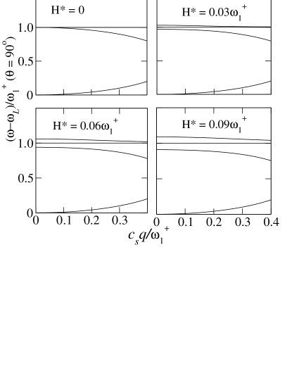
FIG. 1.: Dispersion relations at vanishing temperatures. ${\rm H}^{*}\equiv e|{\bf H}_{0}|(1+F_{0}^{a}/3)/m^{*}$.

The remaining 6 components can be conveniently “folded” onto the complex “vector” ${\bm{j}}^{+}_{\sigma}\equiv\hat{x}\cdot{{\bm{j}}_{\sigma}}_{\alpha}\hat{x}_{\alpha}+i\hat{y}\cdot{{\bm{j}}_{\sigma}}_{\alpha}\hat{x}_{\alpha}$, which measures the transport of transverse magnetization $\delta m^{+}\equiv\delta m_{x}+i\delta m_{y}$ under the driving field $\delta H^{+}\equiv\delta H_{x}+i\delta H_{y}$. Solving Eqs.(12) and (14) for the Fourier components yields[12]

$${\bm{j}}^{+}_{\sigma}=-\frac{\delta H^{+}c_{s}^{2}}{P_{4}(\Omega)}[\gamma |{\bf m}_{0}|-\chi_{0}(\omega-\omega_{L})]$$ (15)

$$\times [\Omega^{2}{\bf q}-i\Omega{\bf H}^{*}\times{\bf q}-({\bf H}^{*}\cdot{\bf q}){\bf H}^{*}],$$ (16)

and ${\delta m}^{+}=-{\delta H}^{+}{\gamma|{\bf m}_{0}|P_{3}(\Omega)}/{P_{4}(\Omega)},$ where $\Omega\equiv\omega-\omega_{L}-z_{0}$, $\omega_{L}$ is the Larmor frequency, $z_{0}\equiv\omega_{1}^{+}-i\omega_{D}^{*}$, $P_{3}(\Omega)=\Omega^{3}+(c_{s}^{2}q^{2}{\chi_{0}}/{\gamma|{\bf m}_{0}|})\Omega^{2}-{{\rm H}^{*}}^{2}\Omega-(c_{s}^{2}{\chi_{0}}/{\gamma|{\bf m}_{0}|})({\bf H}^{*}\cdot{\bf q})^{2},$ $P_{4}(\Omega)=\Omega^{4}+z_{0}\Omega^{3}+(c_{s}^{2}q^{2}-{{\rm H}^{*}}^{2})\Omega^{2}-z_{0}{{\rm H}^{*}}^{2}\Omega-c_{s}^{2}({\bf H}^{*}\cdot{\bf q})^{2},$ and ${\bf H}^{*}\equiv{\rm H}^{*}\hat{z}$. For simplicity we specialize to the case ${\bf H}_{0}\perp{\bf q}$ (indicated by $\theta=90^{o}$ in the figures). This condition is obtained in practice by sheding neutrons or photons adequately on a finite sample’s surface, and is the condition that maximizes the non-chiral orbital contribution in Eq.(16); in the infinite system, we can think of transverse magnons if we wish to quantize the hydrodynamics. Longitudinal magnons will be treated elsewhere.[12] In Fig.(1) we see the dispersion relations for different values of the external field. These are obtained by looking into the free modes ($\delta{\bf H}=0$). It is clear that the degeneracy is only exact at $q=0$. We see also that it constitutes a three-fold degeneracy, however, the two constant branches shown ($\omega-\omega_{L}\equiv\Delta\omega=\omega_{1}^{+}$) are spurious when ${\bf H}_{0}=0$ in the sense that there is no spectral weight associated with them, as seen in Fig.(2) where $S(q,\omega)\propto{\rm Im}[\delta m^{+}/\delta H^{+}]$ (which is the important quantity in experiments) is plotted as a function of $\omega$ and ${\rm H}^{*}$.

   

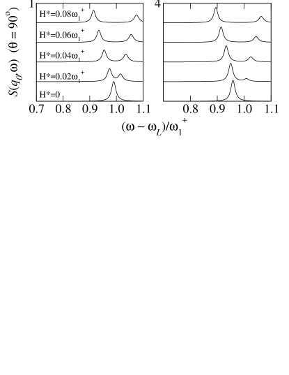
FIG. 2.: Spectral weight in arbitrary units. The splitting is clearly seen as the magnetic field increases. Numbers on the upper left corner give the amplitude of one plot relative to the next. These amplitudes are of order of $10^{-2}$ the (not shown) Goldstone mode amplitudes which do not split under the external field. The curves are translated vertically to facilitate analysis. The values of ${\bf H}^{*}$ correspond to hundreds of Gauss in, e.g., MnSi.

Under a finite magnetic field only one of the spurious branches develops weight while the degeneracy is lifted.

The important point to note is that the frequencies of the Goldstone mode (the traditional spin-waves) only shift their loci as the external magnetic field increases whereas the gapped mode splits. This can be seen in Fig.(3) where the behavior of these dispersions with the external field is shown (including the Goldstone mode). It is then clear that the splitting of the gapped mode should be considered as a distinctive feature in experiments searching for a direct observation of it. It should be helpful to make a statement about the quantities involved for some traditional materials: From data found in the literature we estimate the fields shown to be in the range of hundreds of Gauss for typical weak ferromagnets like MnSi, ZrZn₂, and Ni₃Al. This corresponds to a gap of tenths of meV in these materials.[13]

   

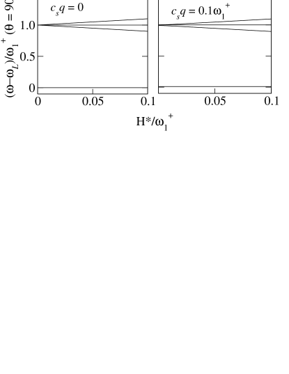
FIG. 3.: Linear behavior of the dispersions with ${\rm H}^{*}$. The effect of ${\rm H}^{*}$ on the Goldstone mode ($\omega-\omega_{L}\sim 0$) is seen to merely shift its frequency.

For small values of ${\rm H}^{*}$ and $q$ (up to $0.1\omega_{1}^{+}$), the dispersions may be put in the simple form $\Delta\omega=c_{s}^{2}q^{2}/\omega_{1}^{+}$ for the Goldstone mode and $\Delta\omega=\pm{\rm H}^{*}+\omega_{1}^{+}-\alpha q^{2}$ for the gapped mode.[14] Quantization of the theory in this limit will yield massive magnons with an “up-down” degeneracy which is lifted by the magnetic field, in much the same way as in the Zeeman effect of a single spin. The possible existence of (low temperature) magnons with mass and a Zeeman-like degeneracy makes room for new questions realated, e.g., to the collective behavior of a handful of these excitations. Before these questions are put forward it is, however, prudent to focus on the issue of whether these results can be observed by traditional experiments. The spectral weight of this mode, of order of $10^{-2}$ the usual spin waves (see Fig.(2)) stands as an obstacle. Our main emphasis here is whence on the additional criterium such a degeneracy provides to track down the massive mode. In a companion longer article we also discuss how these results are expected to show in a conduction ressonance experiment. [12]

The authors aknowledge fruitful discussions with K. Blagoev. Financial support for this work has been provided by DOE Grant DEFG0297ER45636, and FAPESP Grants 01/01713-3, 00/07660-6, and 00/10805-6.

REFERENCES

- [1] F. Bloch, Z. Phys. 31, 206 (1930).
- [2] J.C. Slater, Phys. Rev. 35, 509 (1930).
- [3] R.D. Lowde, Proc. R. Soc. A, 235, 305 (1956).
- [4] L.D. Landau, Soviet Phys. JETP 3, 920 (1956).
- [5] V.P. Silin, Soviet Phys. JETP 6, 945 (1958).
- [6] A.A. Abrikosov and I.E. Dzyaloshinskii, Sov. Phys. JETP 35, 535 (1959).
- [7] I.E. Dzyaloshinskii and P.S. Kondrantenko Sov. Phys. JETP 43, 1036 (1976); I.E. Dzyaloshinskii, private communication.
- [8] K.S. Bedell and K.B. Blagoev, Phil. Mag. Lett. 81, 511 (2001).
- [9] In this article the so called hydrodynamic approximation is used which consists of keeping only the two first spherical harmonics in the expansions of the responses about the Fermi surface. To properly determine one has to go beyond such an approximation , as in Ref.[8], where it has been found (in the absence of an external field) that ( is the density, and the bare and effective masses and the second Landau antisymmetric parameter).
- [10] The fact that the gapped mode does not propagate in the presence of collisions is due to its origin in the oscillations of spin-current, which is not a conserved quantity.[8]
- [11] P.M. Platzman and P. A. Wolff, Phys. Rev. Lett. 18, 280 (1967); see also P.M. Platzman and P. A. Wolff, Waves and Interactions in Solid State Plasmas (Academic Press, New York, 1973).
- [12] P.F. Farinas and K.S. Bedell, in preparation.
- [13] Y. Ishikawa, Y. Noda, Y.J. Uemura, C.F. Majkrzak, and G. Shirane, Phys. Rev. B 25, 254 (1982); N.R. Bernhoeft, G.G. Lonzarich, P.W. Mitcjell, and D. MkK. Paul, Phys. Rev. B 28, 422 (1983).
- [14] For the strict hydrodynamic approximations used here, . A more rigorous expression for the relation between and the Landau parameters in a finite magnetic field will be presented in the future; we do not expect to change, to leading order in the field, from the expression derived in Ref.[8].[9]