Transmission Phase of an Isolated Coulomb–Blockade Resonance

Abstract

In two recent papers, O. Entin–Wohlman et al. studied the question: “Which physical information is carried by the transmission phase through a quantum dot?” In the present paper, this question is answered for an islolated Coulomb–blockade resonance and within a theoretical model which is more closely patterned after the geometry of the actual experiment by Schuster et al. than is the model of O. Entin–Wohlman et al.. We conclude that whenever the number of leads coupled to the Aharanov–Bohm interferometer is larger than two, and the total number of channels is sufficiently large, the transmission phase does reflect the Breit–Wigner behavior of the resonance phase shift.

I Introduction

In 1997, Schuster et al. [1] reported on a measurement of the transmission phase through a quantum dot (QD). These authors used an Aharanov–Bohm (AB) interferometer with the QD embedded in one of its arms. The device is schematically shown in Figure 1. The current through the device is made up of coherent contributions from both arms and is, therefore, a periodic function of the magnetic flux $\phi$ through the AB interferometer. A sequence of Coulomb–blockade resonances in the QD was swept by adjusting the plunger gate voltage $V_{g}$ on the QD. (The plunger gate is not shown in the Figure). The phase shift $\delta\phi$ of the oscillatory part of the current was measured as a function of $V_{g}$. We refer to this phase shift as to the transmission phase through the QD. As expected, $\delta\phi$ showed an increase by $\pi$ over each Coulomb–blockade resonance.

The AB interferometer of Ref. [1] was attached to six external leads. The complexity of this arrangement was caused by the failure of an earlier two–lead experiment [2] also aimed at measuring $\delta\phi$. Instead of a smooth rise by $\pi$ over the width of each resonance, a sudden jump by $\pi$ near each resonance was observed. This feature was later understood to be caused by a special symmetry property of the two–lead experiment [3]: The conductance $g(\phi)$ and, therefore, the current are symmetric functions of $\phi$ and, hence, even in $\phi$. Thus, $g$ is a function of $\cos(\phi)$ only, and the apparent phase jump of $\delta\phi$ by $\pi$ is actually due to the vanishing at some value of $V_{g}$ near resonance of the coefficient multiplying $\cos(\phi)$.

.

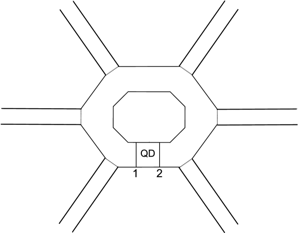
FIG. 1.: An AB interferometer containing a QD in one of its arms and attached to six external leads (schematic). The barriers labelled $1$ and $2$ separate the QD from the AB ring, the dashed lines the AB ring from the leads. Barriers and dashed lines are considered closed in the geometry defining the Hamiltonian $H_{0}$ in Eq. (4).

Following the work of Ref. [1], theoretical attention was largely focused on the least expected feature of the data of Ref. [1]: A sequence of Coulomb–blockade resonances displayed very similar behavior regarding the dependence of both, the conductance and the transmission phase, on $V_{g}$. In particular, $\delta\phi$ displayed a rapid drop between neighboring Coulomb–blockade resonances. For references, see Ref. [4]. It is only recently that Entin–Wohlman, Aharony, Imry, Levinson, and Schiller [5, 6] drew attention to the behavior of $\delta\phi$ at a single resonance. In Ref. [5] the first four authors consider a three–lead situation. Two leads are attached to the AB interferometer in a fashion analogous to Figure 1. The third lead connects directly to the QD. The authors take the arms of the AB interferometer and the three external leads as one–dimensional wires. They consider an isolated resonance due to a single state on the QD. Solving this model analytically, they come up with a disturbing result: The transmission phase increases by $\pi$ over an energy interval given by that part of the width of the QD which is due to its coupling to the third lead. As this coupling is gradually turned off, the rise by $\pi$ of $\delta\phi$ becomes ever more steep, and eventually becomes a phase jump by $\pi$ as the coupling to the third lead vanishes. In Ref. [6], the model is extended to include additional one–dimensional wires directly attached to the AB ring and coupled to it in a special way. Again, it is found that the transmission phase reflects the resonance phase shift only “for specific ways of opening the system”[6]. These results immediately poses the following questions: What is the behavior of $\delta\phi$ for a single resonance in the six–lead case and, more generally, for any number of leads in a geometry like the one shown in Figure 1? Does the rise of $\delta\phi$ by $\pi$ occur over an energy interval given by the actual width of the resonance or only by part of that width? And what happens to $\delta\phi$ as the number of leads is gradually reduced to two? It is the purpose of the present paper to answer these questions within a theoretical framework which is more closely patterned after the experimental situation than is the work of Ref. [5]. In particular, our work differs from that of Refs. [5, 6] in the following respects: We do not assume that the QD is directly coupled to a lead, we do not make any specific assumptions about the way in which the leads are coupled to the AB ring, and we allow for an arbitrary number of leads (as long as this number is at least equal to two) and of channels in each lead.

II Model

In one of the first theoretical papers [8] addressing the data of Ref [1], the transmission phase $\delta\phi$ was calculated in the framework of a model designed in Ref. [7], and for the geometry shown in Figure 1. Inspection of the curves published in Ref. [8] shows that the transmission phase rises roughly by $\pi$ over an energy interval roughly equal to the width of each Coulomb–blockade resonance. The curves shown in Ref. [8] were, however, calculated in the framework of specific assumptions on a number of parameters and do not, therefore, constitute a general answer to the questions raised at the end of Section I. Still, it is useful to employ again the model used in these calculations. As we shall see, the model yields a completely general expression for the conductance and its dependence upon $V_{g}$ and $\phi$ in the framework of the geometry displayed in Figure 1.

Starting point for the study of a case with $R$ leads where $R$ is integer and $R\geq 2$ is the Landauer–Büttiker formula

$$I_{r}=\sum_{s=1}^{R}G_{rs}V_{s}\ .$$ (1)

The formula connects the current $I_{r}$ in lead $r$, $r=1,\ldots,R$ with the voltages $V_{s}$ applied to leads $s$. The conductance coefficients $G_{rs}$ are given by

$$G_{rs}=\frac{e^{2}}{h}T^{rs}=\frac{e^{2}}{h}\sum_{ab}\int{\rm d}{\cal E}\biggl{(}\frac{{\rm d}F({\cal E})}{{\rm d}{\cal E}}\biggr{)}[|S^{rs}_{ab}({\cal E})|^{2}-\delta_{ab}]\ .$$ (2)

Here $S^{rs}_{ab}({\cal E})$ are the elements of the scattering matrix $S$ connecting channel $a$ in lead $r$ with channel $b$ in lead $s$ at an energy ${\cal E}$ of the electron. We have used the terminology of scattering theory and identified the transverse modes of the electron in each lead with the channels. The function $F({\cal E})$ is the Fermi function. We simplify our reasoning by considering very low temperatures where the integral in Eq. (2) can be replaced by $[|S^{rs}_{ab}(E_{F})|^{2}-\delta_{ab}]$, identifying the Fermi energy parametrically with the plunger gate voltage $V_{g}$. We do so because this brings out the energy dependence of the transmission phase most clearly. Subsequent averaging over temperature does not change the essential aspects. We recall that the Landauer–Büttiker formula is restricted to the case of independent electrons. This is the approximation used throughout the paper.

To proceed, we must introduce a model for the scattering matrix $S(E_{F})$. We consider a geometrical arrangement of the type shown schematically in Figure 1 without, however, limiting ourselves to six channels. We emphasize that this geometry differs from the one considered in Ref.[5] where, as mentioned above, the QD is directly coupled to one of the leads. The electrons move independently in the two–dimensional area defined by the leads, the AB interferometer, and the QD. A homogeneous magnetic field is applied perpendicularly to the plane of Figure 1.

The two–dimensional configuration space is divided into disconnected subspaces defined by the interior of the QD, of the AB interferometer without the QD, and by each of the leads. The free scattering states in lead $r$ carry the labels $E$ for energy and $a$ for the channel, with $c^{r\dagger}_{aE}$ and $c^{r}_{aE}$ the corresponding creation and destruction operators. The bound states in the closed AB ring have energies $\varepsilon_{i}$, $i=1,2,\ldots$ and associated operators $d^{\dagger}_{i}$ and $d_{i}$. The QD supports a single bound state with energy $E_{0}$ and associated operators $q^{\dagger}$ and $q$. This last simplification is introduced because we wish to investigate the behavior of $\delta\phi$ at an isolated Coulomb–blockade resonance. At the expense of an increase of the number of indices, this assumption can easily be removed, see Refs. [7, 8].

The single–particle Hamiltonian $H$ is accordingly written as the sum of two terms,

$$H=H_{0}+H_{1}\ .$$ (3)

Here, $H_{0}$ describes free electron motion in each of the disconnected subspaces,

$$H_{0}=\sum_{r,a}\int{\rm d}E\ Ec^{r\dagger}_{aE}c^{r}_{aE}+\sum_{i}\varepsilon_{i}d^{\dagger}_{i}d_{i}+E_{0}q^{\dagger}q\ .$$ (4)

The coupling between the various subspaces, and the influence of the magnetic field are contained in the coupling Hamiltonian

$$H_{1} = \sum_{r,a,i}\int{\rm d}E\biggl{(}W^{r}_{ai}(E)c^{r\dagger}_{aE}d_{i}+h.c.\biggr{)}$$ (6)

$$\qquad+\sum_{ip}\biggl{(}V^{p}_{i}q^{\dagger}d_{i}+h.c.\biggr{)}\ .$$

The matrix elements $W^{r}_{ai}(E)$ describe the coupling between channel $a$ in lead $r$ and the state $i$ in the AB ring. There are no barriers separating the leads from the AB ring. Therefore, the coupling to the leads will change the states $i$ into strongly overlapping resonances. We will accordingly assume later that the resulting terms depend smoothly on energy $E$. We also assume that on the scale of the mean level spacing in the AB ring, the energy dependence of the $W$’s is smooth and, in effect, negligible. The matrix elements $V^{p}_{i}$ describe the coupling between the states $i$ and the state in the QD with energy $E_{0}$. The upper index $p$ with $p=1,2$ distinguishes the two barriers which separate the QD from the AB ring, see Figure 1. In our model, the topology of the AB ring enters via the occurrence of two independent amplitudes for decay of the state with energy $E_{0}$ on the QD into each of the states $i$ of the AB ring. Because of gauge invariance, the entire dependence of $H$ on the applied magnetic field can, without loss of generality, be put into one of the matrix elements $V$. We accordingly assume that the amplitudes $W^{r}_{ai}(E)$ and $V^{1}$ are real and write $V^{2}$ in the form

$$V^{2}_{i}\exp(+i\phi)=(V^{2}_{i})^{*}\exp(-i\phi)=v^{(2)}$$ (7)

where $v^{(2)}$ is real. The phase $\phi$ is given by $2\pi$ times the magnetic flux through the AB ring in units of the elementary flux quantum. Eqs. (6,7) imply that the electron picks up the phase factor $\exp(+i\phi)$ as it leaves the QD through barrier $2$. Here and likewise in Section III, we neglect all other effects that the magnetic field may have on the motion of the electron, and take account of the Aharanov–Bohm phase only.

The Hamiltonian used in Ref. [7] differs from our $H_{0}$ in that it also contains the Coulomb interaction between electrons within the QD in a mean–field approximation. This interaction is known [4] to be important for the behavior of the phase of the transmission amplitude through the QD between resonances. It is not expected, however, to affect this phase in the domain of an isolated Coulomb–blockade resonance, or the width of such a resonance.

III Scattering Matrix

One may wonder whether the model defined in Eqs. (3) to (7) is sufficiently general to give a completely satisfactory answer to the questions posed at the end of Section I. It is for this reason that we now derive the form of the scattering matrix from very general principles. These are unitarity, time–reversal invariance, the topology of the AB interferometer, gauge invariance, and the single–level approximation for the passage of electrons through the QD. As remarked above, the last of these assumptions can easily be lifted. At the end, it will turn out that the scattering matrix determined in this way has indeed the same form as the one calculated from Eqs. (3) to (7).

The total scattering matrix $S$ for the passage of electrons through the AB interferometer is the sum of two terms. We consider first the contribution $S^{(0)}$ from that arm of the interferometer which does not contain the QD. (In the scheme of Figure 1, the total scattering matrix $S(E)$ would become equal to $S^{(0)}(E)$ if the barriers $1$ and $2$ separating the QD from the AB ring were closed). We neglect the dependence of $S^{(0)}$ on energy over an interval given by the width of the resonance due to the single level in the QD in the other arm and, therefore, consider $S^{(0))}$ as independent of energy. Since $S$ is unitary, and since the contribution from the other arm vanishes for energies far from the resonance, $S^{(0)}$ must also be unitary. Moreover, $S^{(0)}$ is not affected by the presence of the magnetic field. (As in the model of Eqs. (3) to (7), the entire dependence on the magnetic field will be contained in the amplitude coupling the QD to the AB ring through barrier $2$, see Eq. (11) below). Hence, $S^{(0)}$ is time–reversal invariant and, thus, symmetric. As is the case for every unitary and symmetric matrix, $S^{(0)}$ can be written in the form [9]

$$S^{(0)}=UU^{T}\ .$$ (8)

The symbol $T$ denotes the transpose of a matrix, and the matrix $U$ is unitary. It is the product of an orthogonal matrix which diagonalizes $S^{(0)}$, and of a diagonal matrix. The elements of the latter have the form $\exp(i\delta)$ where the $\delta$’s are the eigenphaseshifts of $S^{(0)}$. We now use the more explicit notation introduced in Eq. (4) to write $S^{(0)}$ as $(S^{(0)})^{rs}_{ab}$, and $U$ as $U^{r}_{a\alpha}$. With $N_{r}$ the number of channels in lead $r$ and $N=\sum_{r}N_{r}$ the total number of channels, the index $\alpha$ runs from $1$ to $N$. The matrix $U$ represents a rotation in the space of channels from the physical channels $(r,a)$ to the eigenchannels $\alpha$ of $S^{(0)}$.

Using Eq. (8), we write the total $S$–matrix $S$ in the form

$$S^{rs}_{ab}=\sum_{\alpha\beta}U^{r}_{a\alpha}\bigl{(}\delta_{\alpha\beta}-i\frac{x_{\alpha\beta}}{E-E_{0}+(i/2)\Gamma}\bigr{)}U^{s}_{b\beta}\ .$$ (9)

The first term in brackets on the right–hand side of Eq. (9) represents $S^{(0)}$ and the second, the contribution of the single resonance due to the QD. This contribution is written in Breit–Wigner form. The numerator $x_{\alpha\beta}$ has the form

$$x_{\alpha\beta} = z^{(1)}_{\alpha}z^{(1)}_{\beta}+z^{(2)}_{\alpha}z^{(2)}_{\beta}$$ (11)

$$\qquad+z^{(1)}_{\alpha}z^{(2)}_{\beta}\exp(i\phi)+z^{(2)}_{\alpha}z^{(1)}_{\beta}\exp(-i\phi)\ .$$

The amplitudes $z^{p}_{\alpha}$ with $p=1,2$ and $\alpha=1,\ldots,N$ are the amplitudes for decay of the Breit–Wigner resonance into the eigenchannels $\alpha$ through the first or the second barrier, respectively, see Figure 1. The entire magnetic–field dependence is contained explicitly in the phase factors. Therefore, the amplitudes $z^{p}_{\alpha}$ can be chosen real. The four terms on the right–hand side of Eq. (11) account for the four ways in which the Breit–Wigner resonance contributes to the scattering process, see Figure 1: Formation and decay of the resonance through barrier one, formation and decay through barrier two, formation through barrier one and decay through barrier two, and formation through barrier two and decay through barrier one, respectively. Thus, the form of Eq. (11) accounts for the topology of the AB ring and for gauge invariance. In writing Eq. (11), we have assumed that passage through the QD is possible only via intermediate formation of the resonance.

The matrix $S$ in Eq. (9) must be unitary. This condition is met if the total width $\Gamma$ obeys the equation

$$\Gamma = \sum_{\alpha}\sum_{p}(z^{(p)}_{\alpha})^{2}+2\cos(\phi)\sum_{\alpha}z^{(1)}_{\alpha}z^{(2)}_{\alpha}$$ (13)

$$\qquad=\sum_{\alpha}|z^{(1)}_{\alpha}+z^{(2)}_{\alpha}\exp(i\phi)|^{2}\ .$$

The last form of Eq. (13) shows that the amplitude for decay of the resonance into channel $\alpha$ is the sum of two terms, $z^{(1)}_{\alpha}$ and $z^{(2)}_{\alpha}\exp(i\phi)$. Again, this reflects the topology of the AB interferometer. We note that the Breit–Wigner term in Eq. (9) describes both, single and multiple passage of the electron through the QD, the latter possibly in conjunction with multiple turns around the AB ring. This is seen by expanding the Breit–Wigner denominator in Eq. (9) in powers of $\Gamma$, using Eq. (13), and identifying the $n^{\rm th}$ power of pairs of coefficients $z^{(1)},z^{(2)}$ with the $n$–fold passage of the electron through the QD. The expansion gives rise, among many others, for instance to the term

$$(\frac{-i}{E-E_{0}})^{n}(1/2)^{n-1}$$ (14)

$$\times(z^{(1)}_{\alpha}[\sum_{\gamma}z^{(2)}_{\gamma}\exp(+i\phi)z^{(1)}_{\gamma}]^{n-1}z^{(2)}_{\beta}\exp(+i\phi)\ .$$ (15)

With $(-i)$ the propagator in each of the eigenchannels and $(E-E_{0})^{-1}$ the propagator through the resonance on the QD, this term describes an electron passing $n$ times through the QD and circling the AB ring $(n-1)$ times counter–clockwise before leaving the AB device. (The factor $(1/2)^{(n-1)}$ is a matter of convention).

According to Eq. (13), the width $\Gamma$ depends upon the magnetic flux $\phi$. In the context of the question addressed in the present paper, this fact is worrysome. Indeed, what is the meaning of the question “Does the transmission phase increase by $\pi$ over the width of the resonance?” if that width changes with the applied magnetic field? We now show that the dependence of $\Gamma$ on $\phi$ becomes negligible when the total number $N$ of channels becomes large, $N\gg 1$. The amplitudes $z^{(p)}_{\alpha}$ are real but may be positive or negative. For a rough estimate, we assume that the $z$’s are Gaussian–distributed random variables with zero mean value and a common variance $z^{2}$. Then the mean value of $\Gamma$ is easily seen to be independent of $\phi$ and given by $2Nz^{2}$. The variance of $\Gamma$, on the other hand, is given by $[4N^{2}+4N(1+\cos^{2}(\phi))](z^{2})^{2}$. This establishes our claim: The dependence of $\Gamma$ on $\cos(\phi)$ is small of order $1/\sqrt{N}$. To simplify the discussion, we will assume in the sequel that $\Gamma$ is independent of $\phi$.

Inspection shows that the matrix $S$ obeys the identity

$$S(\phi)=S^{T}(-\phi)\ .$$ (16)

This equation expresses time–reversal invariance in the presence of a magnetic field.

For later use, we write, with $f(E)$ real, the Breit–Wigner denominator in the form

$$\frac{1}{E-E_{0}+\frac{i}{2}\Gamma}=f(E)\exp(i\xi(E))\ .$$ (17)

Here, $\xi(E)$ is the resonance phase shift. It increases by $\pi$ over the width $\Gamma$ of the resonance. We recall that we assume $\Gamma$ to independent of $\phi$. The questions raised at the end of Section I amount to asking: “What is the connection between the transmission phase and the resonance phase shift $\xi(E)$?” We will turn to this question presently.

It is useful to introduce the amplitudes

$$\gamma^{r}_{a}=\sum_{\alpha}U^{r}_{a\alpha}z^{(1)}_{\alpha}\ ,\ \delta^{r}_{a}=\sum_{\alpha}U^{r}_{a\alpha}z^{(2)}_{\alpha}\ .$$ (18)

The symbol $\delta^{r}_{a}$ should not be confused with the eigenphaseshift $\delta_{\alpha}$ of $S^{(0)}$. After multiplication with the matrix $U$, the numerator of the Breit–Wigner term takes the form

$$\gamma^{r}_{a}\gamma^{s}_{b} + \delta^{r}_{a}\delta^{s}_{b}+[\gamma^{r}_{a}\delta^{s}_{b}+\delta^{r}_{a}\gamma^{s}_{b}]\cos(\phi)$$ (20)

$$\qquad+i[\gamma^{r}_{a}\delta^{s}_{b}-\delta^{r}_{a}\gamma^{s}_{b}]\sin(\phi)\ .$$

The total scattering matrix is given by

$$S^{rs}_{ab}(E) = (S^{(0)})^{rs}_{ab}-if(E)\exp(i\xi(E))[\gamma^{r}_{a}\gamma^{s}_{b}+\delta^{r}_{a}\delta^{s}_{b}$$ (23)

$$+[\gamma^{r}_{a}\delta^{s}_{b}+\delta^{r}_{a}\gamma^{s}_{b}]\cos(\phi)$$

$$\qquad+i[\gamma^{r}_{a}\delta^{s}_{b}-\delta^{r}_{a}\gamma^{s}_{b}]\sin(\phi)]\ .$$

The width $\Gamma$ can also be expressed in terms of the amplitudes $\gamma^{r}_{a}$ and $\delta^{r}_{a}$,

$$\Gamma=\sum_{ra}|\gamma^{r}_{a}+\delta^{r}_{a}\exp(i\phi)|^{2}\ .$$ (24)

As announced above, we have shown that the scattering matrix $S$ can indeed be constructed from the requirements of unitarity, time–reversal invariance, the topology of the AB interferometer, gauge invariance, and the single–level approximation. Explicit construction of the scattering matrix from the Hamiltonian formulated in Eqs. (3) through (7) as done in Ref. [7] yields an expression which is identical in form to our $S$ in Eq. (23). This shows that our formal construction possesses a dynamical content. Conversely, this result shows that our model Hamiltonian in Eqs. (3) to (7) leads to the most general form of the scattering matrix which is consistent with the requirements just mentioned. We recall that our construction is strictly based upon a single–particle picture and does not account for interactions between electrons beyond the mean–field approximation.

IV The Transmission Phase

Equipped with an explicit expression for $S$, we return to the transmission phase. It should first be noted that different experiments may determine different combinations of the conductance coefficients $G_{rs}$ introduced in Eq. (1). As shown in Ref. [8], the relevant quantity for the experiment of Schuster et al. [1] is $T^{41}/(T^{44}-N_{4})$. Here, the indices $1$ and $4$ label the source and the collector, respectively, for the electrons in the six–lead experiment. We will show presently that $T^{rr}$ with $r=1,\ldots,R$ is an even function of the phase $\phi$ and, therefore, depends only upon $\cos(\phi)$. A non–trivial dependence on $\phi$ involving both $\cos(\phi)$ and $\sin(\phi)$ and, thus, a trigonometric dependence on $(\phi\pm\xi(E_{F}))$, arises only from the terms $T^{rs}$ with $r\neq s$. Without loss of generality we, therefore, focus attention on $T^{12}$ and, thus, on $\sum_{ab}|S^{12}_{ab}(E_{F})|^{2}$, see Eq. (1). This quantity is expected to display a non–trivial dependence on $\phi$. We expect that the transmission phase $\delta\phi$ increases by $\pi$ as the Fermi energy sweeps the Coulomb–blockade resonance. We ask how this increase depends on the width $\Gamma$ of the resonance and on the number $R$ of leads.

It is useful to address these questions by using the unitarity relation. We write

$$\sum_{ab}|S^{12}_{ab}|^{2}=N_{1}-\sum_{ab}|S^{11}_{ab}|^{2}-\sum_{s\geq 3}\sum_{ab}|S^{1s}_{ab}|^{2}\ .$$ (25)

The advantage of Eq. (25) is that the sum over $s$ vanishes when there are only two leads. Thus, the influence of the number of leads is made explicit. We now discuss the dependence of the terms on the right–hand side of Eq. (25) on the resonance phase shift $\xi(E)$.

Each of the terms $\sum_{ab}|S^{1s}_{ab}|^{2}$ with $s=1,3,4,\ldots$ in Eq. (25) is the sum of three contributions, involving $|S^{(0)}|^{2}$, the square of the Breit–Wigner contribution, and the interference term between $S^{(0)}$ and the Breit–Wigner term. The contributions from $\sum_{ab}|(S^{(0)})^{1s}_{ab}|^{2}$ are independent of both, energy and magnetic field and, therefore, without interest. These terms only provide a smooth background. The squares of the Breit–Wigner terms are each proportional to $f^{2}(E_{F})$ and are independent of the resonance phase shift $\xi(E_{F})$. This is expected. Each such term depends on the magnetic flux $\phi$ in two distinct ways. The squares of the terms in Eq. (23) involving either $\cos(\phi)$ or $\sin(\phi)$, and the product of these two terms yield a dependence on $\phi$ which is periodic in $\phi$ with period $\pi$. Such terms can easily be distinguished experimentally from terms which are periodic in $\phi$ with period $2\pi$. As we shall see, it is some of these latter terms which carry the resonance phase shift $\xi(E_{F})$. Therefore, we confine attention to terms of this latter type. A contribution of this type arises from the square of the Breit–Wigner term via the interference of that part of the resonance amplitude which is independent of $\phi$ with the terms proportional to either $\cos(\phi)$ or $\sin(\phi)$. The sum of all such contributions (from values of $s=1$ and $s=3,4,\ldots,R$) has the form

$$f^{2}(E_{F})A\cos(\phi+\alpha_{0})$$ (26)

where $A$ and $\alpha_{0}$ are constants wich depend on $R$ but not on $E_{F}$ or $\phi$. We note that the constant $A$ is of fourth order in the decay amplitudes $\gamma^{r}_{a}$ and $\delta^{r}_{a}$. Isolated resonances in quantum dots require high barriers, i.e., small values of these decay amplitudes. Therefore, the term (26) may be negligible. We continue the discussion under this assumption but note that there is no problem in taking account of this term if the need arises.

We turn to the interference terms. We first address the case $s=1$ which differs from the cases with $s\geq 3$. We observe that $(S^{(0)})^{11}_{ab}$ is even in $a,b$. Therefore, multiplication of $S^{(0)}$ with the Breit–Wigner term and summation over $a$ and $b$ will cancel those parts of the Breit–Wigner term which are odd under exchange of $a$ and $b$. Inspection of Eq. (20) shows that these are the terms proportional to $\sin(\phi)$. As a consequence, the interference term for $s=1$ is even in $\phi$ and a function of $\cos(\phi)$ only. Explicit calculation shows that the term proportional to $\cos(\phi)$ can be written in the form

$$4f(E_{F})x^{(1)}\cos(\phi)\sin(\xi(E_{F})+\zeta^{(1)})\ .$$ (27)

Here, $x^{(1)}$ and $\zeta^{(1)}$ are independent of energy and explicitly given by $x^{(1)}\exp(i\zeta^{(1)})=\sum_{ab}\gamma^{(1)}_{a}\delta^{(1)}_{b}((S^{(0)})^{11}_{ab})^{*}$. We observe that as a function of energy, $\sin(\xi(E_{F})+\zeta)$ always has a zero close to the resonance energy $E_{0}$. When only two channels are open, the entire dependence on $\phi$ which has period $2\pi$ resides in this term. The term does not display the resonance phase shift except through the zero near $E_{0}$. It is symmetric in $\phi$ about $\phi=0$. These facts are well known [3], of course, and are reproduced here for completeness only. The form (27) of the interference term was responsible for the failure of the experiment in Ref. [2] to measure the transmission phase.

For the interference terms with $s\geq 3$, the matrix $(S^{(0)})^{1s}_{ab}$ is not symmetric in $a,b$. (It is symmetric only with respect to the simultaneous interchange of $1,s$ and $a,b$). Therefore, the terms proportional to $\sin(\phi)$ in Eq. (23) do not cancel, and the interference terms acquire a genuine joint dependence on both, the resonance phase shift $\xi(E_{F})$ and the phase $\phi$ of the magnetic flux. Proceeding as in the previous paragraph, we introduce the constants $x\exp(i\zeta)=\sum_{s\geq 3}\sum_{ab}\gamma^{(1)}_{a}\delta^{(s)}_{b}((S^{(0)})^{1s}_{ab})^{*}$ and $y\exp(i\theta)=\sum_{s\geq 3}\sum_{ab}\gamma^{(s)}_{a}\delta^{(1)}_{b}((S^{(0)})^{1s}_{ab})^{*}$. The $\phi$–dependent part of the sum of the interference terms with $s\geq 3$ takes the form

$$2f(E_{F})[x\sin(\phi+\xi(E_{F})+\zeta)+y\sin(-\phi+\xi(E_{F})+\theta)]\ .$$ (28)

This expression depends on $\xi(E_{F})$ in the expected way.

We are now in a position to answer the questions raised at the end of Section I. Whenever the total number $N$ of channels coupled to the AB device is sufficiently large, the resonance width $\Gamma$ becomes independent of magnetic flux. This property can be checked experimentally. It is only in this limit that the statement “The resonance phase shift increases by $\pi$ over the width of the resonance” acquires its full meaning. The limit $N\gg 1$ may, of course, be realised even when the number $R$ of leads is small. We turn to the behavior of the transmission phase. We have shown that there are terms proportional to $f^{2}(E_{f})$ which depend upon $\cos(2\phi)$ but not on $\xi(E_{F})$. The form of these terms was discussed above. For a quantum dot with high barriers, it is expected that these terms are small. The terms periodic in $\phi$ with period $2\pi$ are listed in Eqs. (26) to (28). For a quantum dot with high barriers, we expect that the contribution (26) is small. We focus attention on the remaining terms. These depend on the value of $R$. For $R=2$, the phase dependence is given by the term (27). This term is even in the magnetic flux $\phi$ and has a zero close to the resonance energy $E_{0}$. It does not, however, display the smooth increase of the resonance phase phase shift $\xi(E_{F})$ over the width $\Gamma$ of the resonance. If, on the other hand, the number of leads $R$ is large compared to unity, then it is reasonable to expect that the terms in Eq. (28) are large compared to the term in Eq. (27). This is because the number of contributions to the terms in Eq. (28) is proportional to $R-2$. In this case, the transmission phase faithfully reflects the energy dependence of the resonance phase shift $\xi(E_{F})$. Deviations from this limit are of order $1/(R-2)$. As we gradually turn off the coupling to the leads $s$ with $s\geq 3$, the terms (28) gradually vanish. Nevertheless, it is possible — within experimental uncertainties that become ever more significant as the terms (28) become smaller — even in this case to determine the resonance phase shift $\xi(E_{F})$ from the data on the transmission phase. We propose the following procedure. Add formulas (27) and (28) and fit the resulting expression to the data. This should allow a precise determination of $\xi(E_{F})$ and of $\Gamma$ also in cases where the coupling to the leads $s$ with $s\geq 3$ is small. This statement holds with the proviso that the number of channels must be large enough to allow us to consider the total width $\Gamma$ as independent of $\phi$. Whenever the coupling to the leads $s$ with $s\geq 3$ is small, the energy dependence of the transmission phase is quite different from that of the resonance phase shift. Nevertheless, the transmission phase $\delta\phi$ does reflect the energy dependence of the resonance phase shift $\xi$ whenever the number of leads is larger than two. In particular, this energy dependence is governed by the total width $\Gamma$.

In conclusion, we have seen that in a theoretical model which is more closely patterned after the geometry of Figure 1 than is the model of Ref.[5], the transmission phase does reflect the value of the total width. This statement applies whenever the number of leads exceeds the value two, and whenever the total number of channels is large compared to one. Both conditions are expected to be met in the experiment of Schuster et al. [1].

Acknowledgment. I am grateful to O. Entin–Wohlman, A. Aharony, and Y. Imry for informative discussions which stimulated the present investigation. I thank O. Entin–Wohlman for a reading of the paper, and for useful comments. This work was started when I was visiting the ITP at UCSB. The visit was supported by the NSF under contract number PHY99-07949.

REFERENCES

- [1] R. Schuster, E. Buks, M. Heiblum, D. Mahalu, V. Umansky, and H. Shtrikman, Nature 385 (1997) 417.
- [2] A. Yacoby, M. Heiblum, D. Mahalu, and H. Shtrikman, Phys. Rev. Lett. 74 (1995) 4047.
- [3] M. Büttiker, Phys. Rev. Lett. 57 (1986) 1761.
- [4] R. Baltin, Y. Gefen, G. Hackenbroich, and H. A. Weidenmüller, Eur. Phys. J. B 10 (1999) 119.
- [5] O. Entin–Wohlman, A. Aharony, Y. Imry, and Y. Levinson, cond-mat/0109328, and private communication.
- [6] O. Entin–Wohlman, A. Aharony, Y. Imry, Y. Levinson, and A. Schiller, cond-mat/0108064.
- [7] G. Hackenbroich and H. A. Weidenmüller, Phys. Rev. B 53 (1996) 16379.
- [8] G. Hackenbroich and H. A. Weidenmüller, Europhys. Lett. 38 (1997) 129.
- [9] H. Nishioka and H. A. Weidenmüller, Phys. Lett. 157 B (1985) 101.